
Peter Dittrich, Thomas Kron and Wolfgang Banzhaf (2003)
On the Scalability of Social Order: Modeling the Problem of Double and Multi Contingency Following Luhmann
Journal of Artificial Societies and Social
Simulation
vol. 6, no. 1
To cite articles published in the Journal of Artificial Societies and Social
Simulation, please reference the above information and include paragraph
numbers if necessary
<https://www.jasss.org/6/1/3.html>
Received: 14-Jun-2002 Accepted: 9-Jan-2003 Published: 31-Jan-2003
 Abstract
|
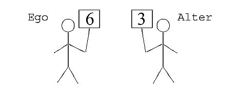
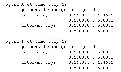
| Figure 1. Two agents interact by showing signs symbolizing messages. |
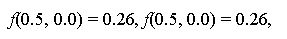
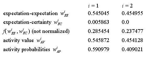
1. For each possible activity 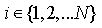 compute:
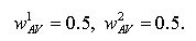
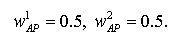
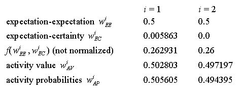
(a) expectation-expectation2. activity probabilities wAP=g(wAV)
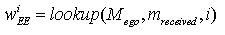
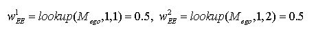
Here, an agent estimates the probability that Agent B expects activity i to be performed next by Agent A. The value is determined by accessing A's memory Mego which has stored responses of Agent A to activities of Agent B. mreceived is the last activity of Agent B to which Agent A has to respond now. In other words, mreceived is the number that Agent B displays on its sign. Roughly speaking, the function lookup(Mego, mreceived, i) returns how often Agent A has reacted with activity i to activity mreceived in the past. In order to model forgetting, past events long passed are counted less than recent events (see Section 2.12, below).(b) expectation-certainty
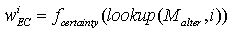
In order to calculate the certainty of the future, Agent A possesses a second memory Malter, which stores how the other agent has reacted to A's activities. So, using this memory, A can predict what B might do as a response to A's potential activity i. Consulting A's alter-memory by calling the function lookup(Malter, i) results in a vector (p1, ...,pN) containing N values. A value pj ∈ [0; 1] of this vector is an estimate of the probability that Agent B responds with activity j to activity i of Agent A. The expectation-certainty is measured by the function fcertainty. The input of that function is the vector (p1,...,pN). The function fcertainty returns a certainty of 0.0, if all values of the vector are the same, e.g., (1/N, 1/N, ..., 1/N), since in that case the agent has no information (there is no distinction possible). The highest certainty (value 1.0) is returned for a vector that consists of zeros but a single value 1, e.g., (1, 0, 0, ..., 0). For this work we measure the certainty by the Shannon entropy (Shannon and Weaver 1949):
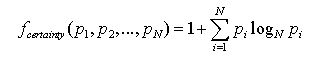
(1) (See Section 9.5 in the Appendix for alternative certainty measures.)
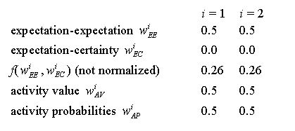
(c) activity value
The expectation-expectation wiEE and the expectation-certainty wiEC are combined by function f and the result is normalized in order to calculate the activity value wiAV. The parameter α specifies the fraction of EC contained in the activity value. f is a linear sum plus a small additive constant:
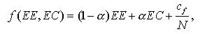
(2) with cf being a constant parameter. The addition of cf / N prevents an activity value from approaching zero in order to avoid artefacts. Division by N assures that the influence of the constant summand does not increase with increasing N. For the experiments presented here we have chosen cf = 0.01 so that there is always at least a small chance for each activity to be selected. In a situation where an agent is rather sure what to do and proportional selection (explained below) is used, there is a chance of about 1% that an activity is selected different from the most probable one. In case of quadratic selection (γ= 2) the "error" probability caused by cf is about 0.2%. (See Section 9.1 in the Appendix for a detailed discussion of cf.)
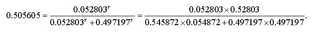
The activity values are scaled by the selection function g: RN → RN:3. Randomly select activity i such that the probability of activity i is wiAP
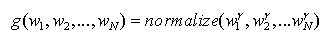
(3) The parameter γ allows to control the influence of randomness (see below). Note that y is an exponent in Eq. (3).

|
| (4) |
|
| (5) |
 |
| (6) |
In order to simplify the following formalism we define a function which returns a vector of all estimated probabilities for every possible response to message a:

|
| (7) |
The Simple Neuronal Memory
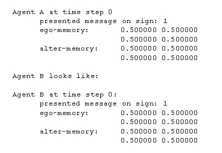
Representation: A memory M is represented by a dimensional matrix ma,b called memory matrix. This matrix (ma,b) is manipulated by the following initialization, memorization and lookup procedures:Initialization: The matrix is initialized with (ma,b) = 1/N.
Memorize(M, a, b): First, we increase the entry in the memory matrix given by the index (a, b) by the learning rate rlearn [7]:
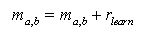
(8) Then we increase all entries by the forgetting rate rforget divided by the number of activities N:
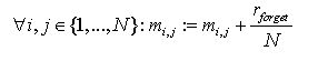
(9) Finally we normalize every line of the memory matrix:
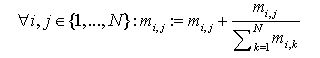
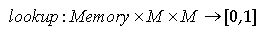
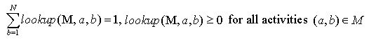
(10) Lookup(M, a, b): Return the entry of the memory matrix given by index (a, b):
(11)
|
|
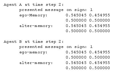
Second, the expectation-certainty is calculated by using the alter-memory:
|
|
and the result is normalized to arrive at the activity values:
|
 |
|
 |
|
|
| (12) |
|
 |
In the dyadic situation (two agents) order appears for a wide range of parameter settings.
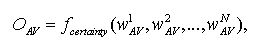 (13) (13)
|
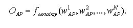 (14) (14) |
In the following we will use OAV only, since it is very similar to OAP and because OAP taking into account has not lead to different conclusions. (OAV and OAP data can be found in log-file: runName.log)
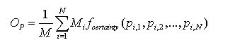 (15) (15)
|
where pi,j is the probability that a randomly drawn agent reacts with activity j to the displayed message i of Alter. Mi is the number of agents displaying message i. The matrix (pi,j) can be interpreted as the average behavior matrix of the whole population. In order to get an intuitive understanding of the systems level order imagine the following game: An external player has to predict the activity of the agents. At the outset the player can take a look at the internal state of every agent. Then, in each turn, an agent is chosen randomly, the activity number i on his sign is shown to the player. (Note that the agents are anonymous, so that the player does not know which agent possesses what kind of internal state). Then, again an agent is chosen randomly from the population and the player has to predict the reaction of that agent to the activity number i. For each correct prediction the player receives a point. The state of the agents is not altered during the game, so they are not allowed to learn during the game. The larger the systems level order OP is, the higher is the maximum average score that the player can achieve. For OP = 0 the player cannot perform better than just guessing randomly. For OP = 1 the player can predict the reaction correctly in each turn. Note that this measure makes sense only if the number of agents is large compared to the number of messages actively used. Sociologically we can interpret the value OP as a measure of integration. Integration with regard to the whole society, "social integration", is a very important term in sociological theory even if it is not definitely clear what it means, because the integration of society could be observed from different analytical perspectives (Münch 1997). The core of social integration consists of a situation of society where all of its particles are stably affiliated with each other and build up a unit which is marked-off outwards. So, in modern societies on the one hand we can differentiate between economical integration, the accentuation of exchange, free contracts, and the capitalistic progression of wealth; political integration, the accentuation of the importance of the exertion of political enforcement by means of national governance; cultural integration, the accentuation of compromise by discourse on the basis of mutually shared reason; and solidarity integration, the accentuation of the necessity of modern societies to generate free citizenships in terms of networks of solidarity. On the other hand we can observe the systemic integration (Schimank 1999). The accentuation here lies on the operational closure of the system.[9] If a (activity) system is operationally closed it is in the position of being able to accept highest complexity of its environment, to pick up and to process this complexity in itself without to imperil its existence. We interpret the value OP as a measure of systemic integration in this sense. In all our simulation experiments a high value of OP has indicated a closure of the emerging activity system. This means that the better the agents are able to predict the activities of other agents as reactions to their own activity selections, the more the communication system appears to be operationally closed, that is certain activities follow certain activities.
|
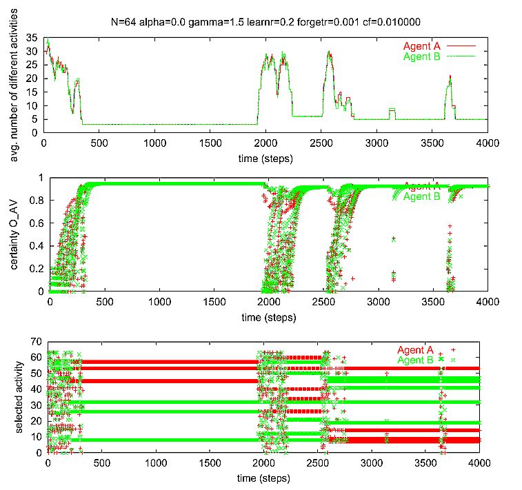
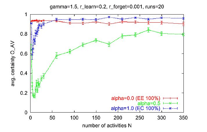
| Figure 2. A complex example of a single run of the dyadic situation. There are N = 64 potential activities. The agents are using expectation-expectation only (a = 0.0). The selection method is something in between proportional and quadratic selection (γ = 1.5). Learning rate rlearn = 0.2. Forgetting rate rforget = 0.001. cf = 0.010000. |
|
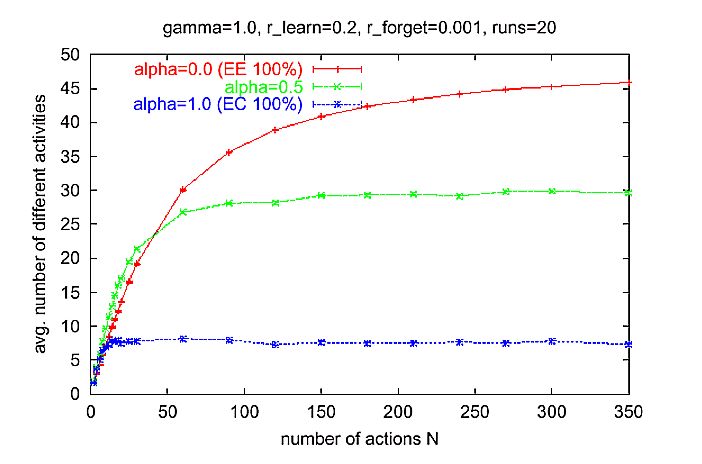
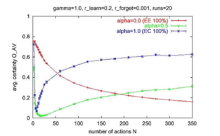
| Figure 3. Average number of different activities in an interval of 50 time steps for different N. Measurement started at time 500 after the transient phase at the beginning. Simulation time: 1000 time steps for each run. Parameter setting: normal learning rate rlearn = 0.2, low forgetting rate rforget = 0.001, proportional selection y = 1. |
|
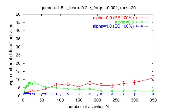
| Figure 4. Same as in Figure 3, but with a lower influence of randomness (y = 1.5). |
Influence of the Selection Method y and EE-EC Factor a
|
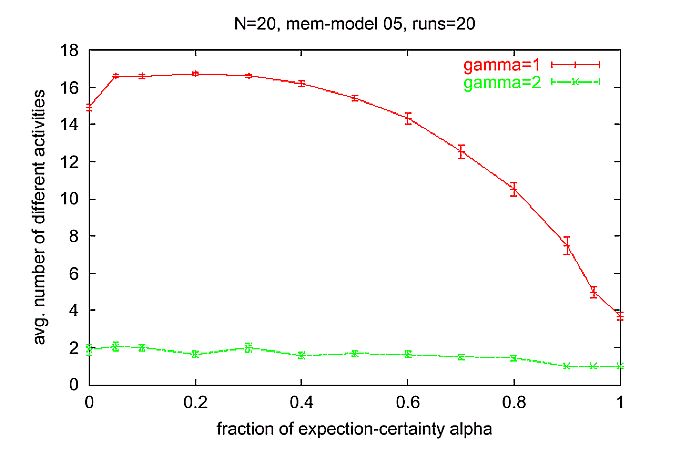
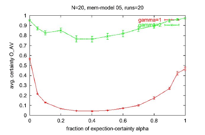
| Figure 5. Average number of different activities in an interval of 50 time steps for different a. Measurement started at time step 500, such that the transient phase at the beginning is not considered. Simulation time 1000 time steps for each run. Parameter setting: normal learning rate rlearn = 0.2, low forgetting rate rforget = 0.001, number of activities N = 20. |
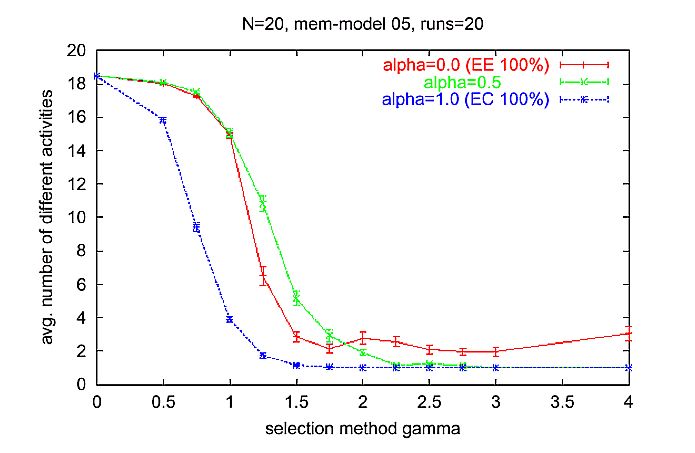 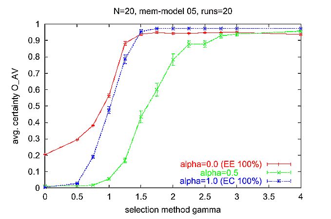 |
| Figure 6. Average number of different messages (activities) in an interval of 50 time steps for different y. Measurement started at time step 500 after the transient phase at the beginning of runs. Simulation time 1000 time steps for each run. Parameter setting: normal learning rate rlearn = 0.2, low forgetting rate rforget = 0.001, number of activities N = 20. |
|
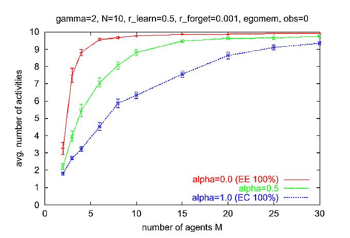
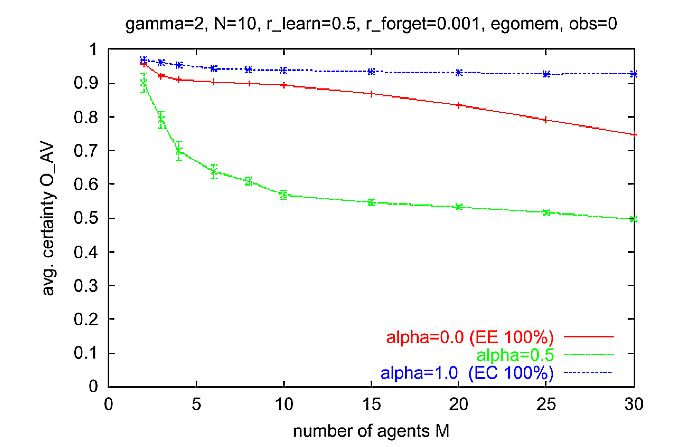
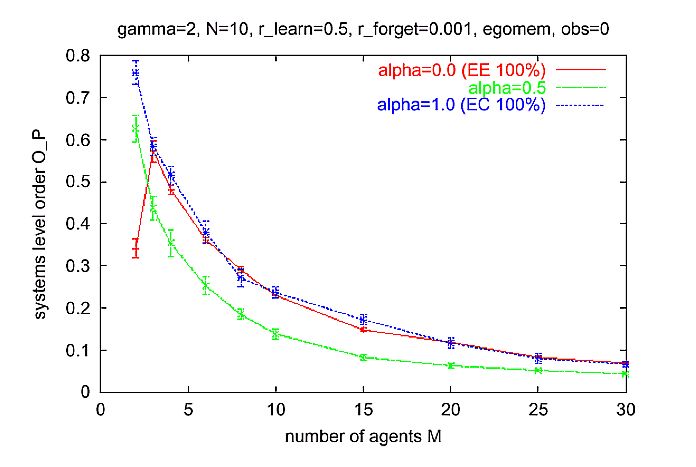
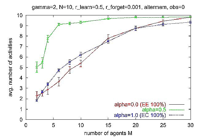
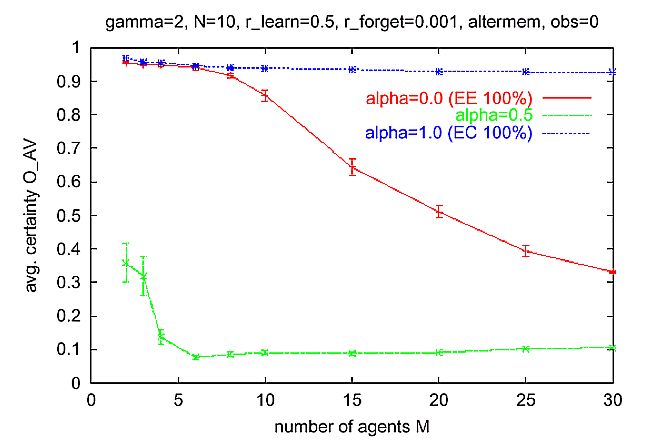
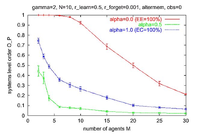
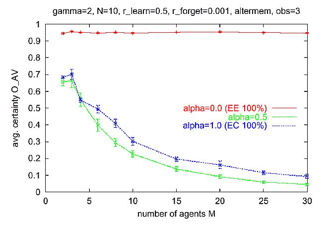
| Figure 7. Average behavior of multi-agent simulations where the Ego-memory is used for calculation of the expectation-expectation, as in the basic dyadic scenario. Parameters: N = 10 activities, y = 2 (quadratic selection), rlearn = 0.5, rforget = 0.001, cf = 0.01. Multi agent scenario as described in Section 6.1 |
|
| Figure 8. Same as Figure 7, but Alter-memory is used to calculate expectation-expectation (EE). Multi-agent scenario as described in Section 6.1. |
In each simulation step, do:
- Randomly choose an agent and call it Ego.
- Randomly choose another agent and call it Alter.
- Let Ego observe Alter's displayed message a (equal to Alter's last activity).
Let Ego reacts to Alter's message. (Note that only Ego acts, but not Alter.)- Ego stores its reaction b in its Ego-memory.
Formally, Ego does: Mego := memorize(Mego, a, b).- Alter stores Ego's reaction b in Alter's Alter-memory.
Formally, Alter does: Malter := memorize(Malter, a, b).- Choose n agents randomly and call them observers.
- Each observer stores Ego's reaction in its Alter-memory.
Formally, each observer performs Malter := memorize(Malter, a, b) where a is the message displayed by Alter and b is Ego's reaction.
|
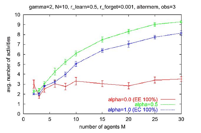
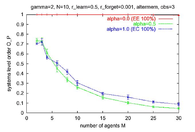
| Figure 9. Same as Figure 8, but with n = 3 observers. For a = 0 (EE only), systems level order is scalable. As in Figure 8, the Alter-memory used to calculate the expectation-expectation. Multi-agent scenario as described in Section 6.13. |
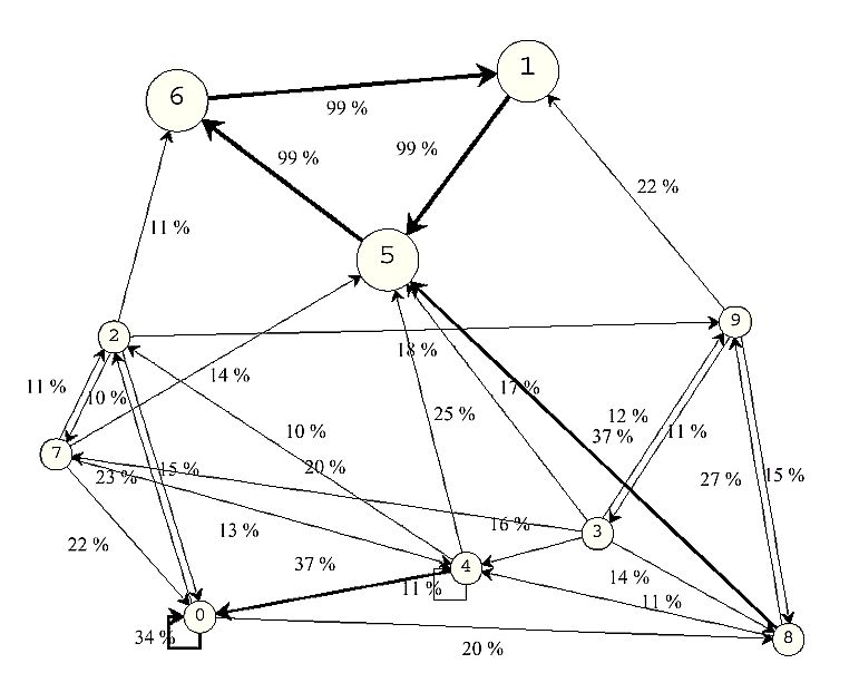
An activity system consists of a set of activity symbols[14] (subset of {1, 2, ..., N}) where activity symbols within that set mainly produce activity symbols within that set, and every activity symbol in that set is produced by activity symbols of that set. This can be expressed more formally[15], e.g.: The set O,O ⊆ {1,2,...N}, is called activity system, if and only if (1) for all v1∈O and v2 ∉O,w(v1, v2) ≤ r, (property of closure), and (2) for all v2∈O there exists v1∈O such that w(v1, v2) > r (property of self-maintenance).
|
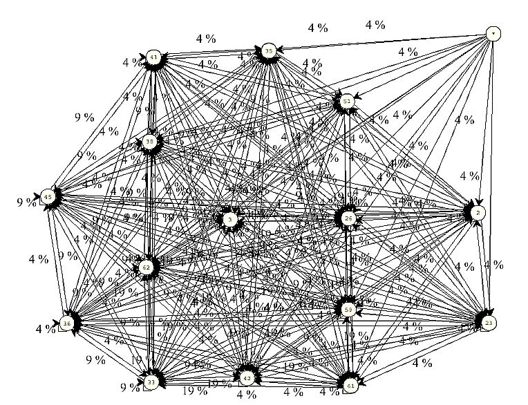
| Figure 10. Typical activity system that has emerged in a simulation experiment with 20 agents, 64 possible activities, and no observers. A node represents an activity. All nodes without any incoming edges are removed, except for one (upper right corner of the diagram), which should illustrate how the removed nodes are connected to the "inner" active network. Parameters: y = 2, N = 64, a = 1:0; rlearn = 0.2, rforget = 0.001, M = 20. No observers. Ego-memory used for EE calculation. Threshold = 0.01. The corresponding single run is shown in the Appendix, Figure 13. |
|
| Figure 11. Example of an activity system that has emerged in a simulation experiment with 10 agents, 10 possible activities, Alter-memory used for EE calculation, and no observers. A node represents an activity. The sub-set of nodes {1, 5, 6} can be interpreted as an autopoietic (sub-)system. Parameters: y = 2, N = 10, a= 0.0, rlearn = 0.2, rforget = 0.001, M = 10. No observers. Alter- memory used for EE calculation. Edges with weights smaller than r = 10% have been omitted for clarity. The corresponding single run is shown in the Appendix |
Is there Autopoiesis?
2 The term "entity" denotes what Luhmann (1988) called "Ego" and "Alter" in Chapter 3 (p. 148), and Parsons called "actor".
3 One of Luhmann's basic assumptions is that both actors are interested in solving this problem. Luhmann (1984, p. 160): "No social system can get off the ground, if the one who begins with communication, cannot know or would not be interested in whether his partner reacts positively or negatively." But the question remains: Where does the motivation (interest) come from? According to Luhmann, an answer should not consider actor characteristics (like intentions) as starting point for system theory. We think that Luhmann falls back to his earlier anthropological position (see Schimank (1988, p. 629; 1992, p. 182)) and assumes a basic necessity of "expectation-certainty", that is, that Alter and Ego want to know what is going on in this situation. A fundamental uncertainty still remains and takes further effect in the emerged systems as an autocatalytic factor. See also the approach to formulate "double contingency" from the perspective of a communication network as provided by Leydesdorff (1993, pp. 58f.)
4 For new simulation experiments about the genesis of symbolic generalized media, see Papendick / Wellner (2002).
5 We prefer to use the term "activity" because Luhmann's concept of communication is much more complex than the communication processes among the agents in our model; see also Hornung (2001). We cannot use the term "action" as understood by Parsons, because our agents do not show a meaningfully motivated behavior that is oriented toward other agents according to certain goals, means, and a symbolic reference framework rooted in the situation. Therefore, our agents decide to do something we call "activity" - no more and no less. For Luhmann every communication consists of a selection triple based on the three distinctions (1) information, (2) transmission (German: Mitteilung), and (3) understanding (see Luhmann (1984, Chapter 4)). Our agents do not communicate in that sense, but we could take their interaction as an abstract model of communication dispensing from the distinction between message, information and meaning. Since it just represents the transmission of information, it is not a accurate model for Luhmann's communication concept. In this contribution, however, we are just interested in the process of order formation and have removed many details for the sake of simplicity.
6 Storing an event (a, b) in memory M is achieved by calling M':= memorize(M, a, b). M' is the new memory (or the new state of the memory), which is created by inserting (a, b) into M.
7 With increasing learning rate, the number of different messages, used by the agents, decreases (see Section 9.2 in the Appendix). Qualitatively, the relative behavior of the model is independent of the choice of the learning rate (above 0.2).
8 Alternatively we can measure the number of different activity- reaction pairs (a, b) occurring in a time interval.
9 Another important meaning of systemic integration in sociology is the integration of different social systems within society.
10 Note that in our simulation there is always a small chance for every activity to be selected.
11 "More or less randomly" means that there are some very small memory traces left. Thus the reaction is not fully dictated by chance. Note also that when we add expectation-certainty the situation will be different.
12 Recall that high systems level order means that just by observing the interactions among (non-learning) agents, it is possible to predict, how an agent in the population will react, without knowing his internal state nor his identity.
13 This non-linearity is not a general phenomenon, because it does not appear if using a different memory type like the linear degenerating memory (type 04), see Appendix Section 9.4.
14 Activity symbols are equivalent to an activity.
15 Note that we define "activity system" operationally for the purposes of our discussion here. The definition should show what can be interpreted as an activity system in our model. And the formal form should make that as clear as possible. It is, however, not a general definition of "activity system".
16 Here, "entity" refers to Ego and Alter in Luhmann's (1984) explanation of the situation of double contingency. Note that an "entity" needs not to be a human person.
17 In terms of Hempel and Oppenheim (1948).
CONTE, R. / M. PAOLUCCI (2001). Intelligent social learning. In: Journal of Artificial Societies and Social Simulation 4 (1): pp. U61-U82.
DITTRICH, P., J. Ziegler, and W. Banzhaf (2001). Artificial chemistries - a review. Artificial Life 7(3), 225-275.
DURKHEIM, E. (1893). De la division du travail social. Paris (1968).
ESSER, H. (1993). Soziologie. Allgemeine Grundlagen. Frankfurt/Main: Campus.
ESSER, H. (2000). Soziologie. Spezielle Grundlagen. Band 2: Die Konstruktion der Gesellschaft. Frankfurt/Main: Campus.
ESSER, H. (2001). Soziologie. Spezielle Grundlagen. Band 6: Sinn und Kultur. Frankfurt/Main: Campus. FONTANA, W. / L. W. BUSS (1996). The Barrier of Objects: From Dynamical Systems to Bounded Organization. In: J. Casti / A. Karlqvist (Eds.), Boundaries and Barriers, Redwood City, MA. Addison- Wesley: pp. 56-116.
FUCHS, S. (2001). Networks. In: Soziale Systeme 7 (1): pp. 125-155.
HEMPEL, C. G. / P. OPPENHEIM (1948). Studies in the logic of explanation. In: Philosophy of Science 15: pp. 135-175.
HOBBES, T. (1651). Leviathan. In: W. Molesworth (Ed.), Collected English Works of Thomas Hobbes, No 3, (1966). Aalen.
HORNUNG, B. R. (2001). Structural coupling and concepts of data and information exchange: Integrating Luhmann into Information Science. In: Journal of Sociocybernetics 2 (2): pp. 13-26.
IKEGAMI, T. / M. TAIJI (1999, September 13-17). Imitation and Cooperation in Coupled Dynamical Recognizers. In D. Floreano / J.-D. Nicoud / F. Mondada (Eds.), Proceedings of the 5th European Conference on Advances in Artificial Life (ECAL-99), Volume 1674 of LNAI, Berlin. Springer: pp. 545-554.
KRON, T. and P. Dittrich (2002).
Doppelte Kontingenz nach Luhmann: Ein Simulationsexperiment.
In: T. Kron (Ed.), Luhman modelliert.
Ansaetze zur Simulation von Kommunikationssystemen,
pp. 209-251. Leske + Budrich, Opladen.
LEPPERHOFF, N. (2000). Dreamscape: Simulation der
Entstehung von Normen im Naturzustand mittels eines computerbasierten Modells des
Rational-Choice-Ansatzes. In: Zeitschrift fr Soziologie 29 (6): pp. 463-
484.
LEYDESDORFF, L. (1993). "Structure" / "Action"
Contingencies and the Model of Parallel Processing. In: Journal for the Theory of
Social Behaviour, 23: pp. 47-77.
LOMBORG, B. (1996). Nucleus and shield: The
Evolution of Social Structure in the Iterated Prisoner's Dilemma. In: American
Sociological Review 61 (2): pp. 278-307.
LUHMANN, N. (1984). Soziale Systeme.
Grundri einer allgemeinen Theorie. Frankfurt a.M.: Suhrkamp.
LUHMANN, N. (1988). Die Wirtschaft der
Gesellschaft. Frankfurt/Main: Suhrkamp.
LUKSHA, P. O. (2001). Society as a Self-Reproducing
System. In: Journal of Sociocybernetics 2 (2): pp. 13-26.
MNCH, R. (1986). The American Creed in Sociological
Theory: Exchange, Negotiated Order, Accommodated Individualism and Contingency.
In: Sociological Theory 4: pp. 41-60.
MÜNCH, R. (1997). Elemente einer Theorie der
Integration moderner Gesellschaften. In: W. Heitmeyer (Ed.), Was h‰lt die
Gesellschaft zusammen? Bundesrepublik Deutschland. Auf dem Weg von der
Konsens- zur Konfliktgesellschaft, Band 2, Frankfurt/Main. Suhrkamp: pp. 66-
109.
PAPENDICK, S. / J. Wellner (2002). Symbolemergenz
und Strukturdifferenzierung. In T. Kron (Ed.), Luhman modelliert. Sozionische
Ans‰tze zur Simulation von Kommunikationssystemen, Opladen. Leske +
Budrich: pp. 175-208.
PARSONS, T. (1937). The Structure of Social
Action. New York: Free Press.
PARSONS, T. (1951). The Social System. New
York: Free Press.
PARSONS, T. (1968). Interaction. In: D. L. Sills (Ed.),
International Encyclopedia of the Social Sciences, Volume 7, London, New
York: pp. 429-441.
PARSONS, T. (1971). The System of Modern
Society. Englewood Cliffs.
SCHIMANK, U. (1988). Gesellschaftliche Teilsysteme
als Akteurfiktionen. In: Kölner Zeitschrift fr Soziologie und
Sozialpsychologie 4: pp. 619-639.
SCHIMANK, U. (1992). Erwartungssicherheit und
Zielverfolgung. Sozialität zwischen Prisoner's Dilemma und Battle of the Sexes. In:
Soziale Welt 2: pp. 182-200.
SCHIMANK, U. (1999). Funktionale Differenzierung
und Systemintegration der modernen Gesellschaft. In J. Friedrichs / W. Jagodzinski
(Eds.), Soziale Integration, Opladen, Wies-baden. Westdeutscher: pp. 47-
65.
Shannon, C. E. / W. Weaver (1949). The Mathematical Theory of
Communication. Urbana: University of Illinois Press.
SKYRMS, B. / R. PEMANTLE (2000). A Dynamic Model
of Social Network Formation. In: Proc. Natl. Acad. Sci. USA 97 (16): pp.
9340-9346.
SMITH, A. (1776). The Wealth of Nations. New
York (1937).
SPERONI di Fenizio, P., P. Dittrich, J. Ziegler, and W. Banzhaf (2000).
Towards a theory of organizations.
In: German Workshop on Artificial Life (GWAL 2000), Bayreuth, 5.-7. April,
2000 (in print).
TAIJI, M. / T. IKEGAMI (1999). Dynamics of Internal
Models in Game Players. In: Physica D 134 (2): pp. 253-266.
 Return to Contents of this issue
© Copyright Journal of Artificial Societies and Social Simulation, [2003]
