
 Abstract
- This paper presents an agent-based model aiming to shed light on the potential destabilizing effects of bank behavior. Our work takes its motivation from the effects of the financial crisis which erupted in 2007 in the US. It draws on the Financial Instability Hypothesis by Hyman P. Minsky, and on the Agent Based macro modeling literature (Delli Gatti et al. 2010, Riccetti et. al 2013) to model a simplified economy in which heterogeneous banks and firms interact on game theoretic rules. Simulation results suggest that aggregate financial instability may emerge as the outcome of banks’ attempt to increase their profit or market share through their pricing strategies. A further finding from the model is the need for banks to take into account time consistency when issuing credit in order to protect the financial stability of the system.
- Keywords:
- Agent Based Modeling, Credit Networks, Financial Stability
Introduction
- 1.1
- The crisis which erupted in 2007 in the U.S. sub-prime mortgage sector, and which soon became a global financial crisis, came unexpectedly for most economists. As such it exposed the need for changes, and evolution in the profession.
- 1.2
- This paper, from both a theoretical and a methodological perspective, relies on streams of literature, which, since the crisis, have been increasingly regarded as valid alternatives to the current mainstream in economics[1]. In particular we present an Agent Based model approach (see Tesfatsion 2006; Delli Gatti et al. 2010b; Farmer &Foley 2009, among many others) illustrating the potentially destabilizing role of banks profit-seeking behavior, as described by the Financial Instability Hypothesis (henceforth FIH) by Hyman P. Minsky (1986, 1992). The financial crisis has highlighted the FIH as a theoretical explanation of the process of evolution from a period of apparent financial stability, as was the Great Moderation, to a period of financial and economic crisis, in this case the Sub-Prime crisis and the Great Recession. According to this theory, prolonged periods of economic growth lead economic agents, mainly firms and banks, to develop optimistic expectations and hence to undertake increasingly riskier financial positions when financing investment; in other words "stability […] is destabilizing" (Minsky 1976, p.11). This path to financial instability was described by Minsky referring to his taxonomy of financial positions, which classifies firms as hedge, speculative and Ponzi, according to the ratio between proceedings and the outflow of money determined by debt and interest repayment. The increasing amount of Ponzi units makes the whole economic system unstable, and eventually leads to a financial crisis, which spreads through the economy due to the inter-correlation between balance sheets. Finally, without an intervention by the State, the financial crisis may become a disruptive economic crisis via debt-deflation and a fall in investment due to pessimistic expectations. Minsky therefore put forward a theory of financial instability centred on investment financing and on the relation between banks and firms. It is well known that the recent financial crisis started in the mortgage market and, after banking sector, affected primarily the households sector. The FIH is widely considered as a valid theoretical framework for the understanding of the sub-prime crisis. Because even though it occurred in a different sector from the one envisaged by Minsky, it bore the core of the dynamic described by the FIH. In particular, the role played by banks is key in our work. Banks are arguably the core sector in the FIH, as, the amount of credit they issue, determines the level of indebtedness of the economic system. Sharing the same pro-cyclical "expectational climate" (Minsky 1986, p.255) of the other agents, they fuel the upward phase of the business cycle, while cutting credit during recessions. Banks are described by Minsky as very active units,[2] whose profit-seeking behavior can lead to financial instability. Minsky indeed defined banking as an "endogenous destabilizer" (Minsky 1986, p.279).
- 1.3
- The potentially destabilizing role of banks has been studied elsewhere referring to the concept of financial accelerator. According to Bernanke et al. (1996), the higher costs imposed to the real economy by the financial sector account for one of the possible explanations for the evolution from shock to crisis. The financial accelerator literature (see also Bernanke &Gertler 1989, 1990; Bernanke &Blinder 1988, 1992), however, relies mainly on representative agent methodology. As underlined by Delli Gatti et al. (2010a), this leads to unsatisfactory results, for three main reasons. First, in the representative agent approach, the shock is uniform across agents, while in the real world an idiosyncratic shock may lead to financial distress (Gabaix 2011). The representative approach ignores coordination problems as well as communication and interaction among individuals. In this kind of models, interaction among agents takes place only through the price mechanism, and for this to be accurate complete information must be assumed (Delli Gatti et al. 2007). Second, as shown by Delli Gatti et al. (2010a) heterogeneity among agents is a key element in explaining the pro-cyclicality of financial fragility at the aggregate level (as it is in the FIH): during a period of growth, the financial robustness of certain units may rise due, for example, to higher profits – in other words they might have anti-cyclical financial fragility – while others may get increasingly indebted in the attempt to capitalize economic growth, and hence exhibit a pro-cyclical financial fragility. The failure of a unit may exert negative effects on the other units and therefore cause (pro-cyclical) higher financial fragility at the aggregate level. There is therefore no need for the leverage to rise at the aggregate level in order to experience higher systemic financial fragility. This also allows the aggregation problems of the FIH to be overcome (Lavoie &Seccareccia 2001).
- 1.4
- This leads to the third and final point raised by Delli Gatti et al. (2010a): networks are a key element of the financial accelerator. The failure of a firm has a negative impact on its creditors' balance sheets and these creditors, mostly the banks, may impose worse credit conditions on their other borrowers, hence propagating financial distress through its credit network. In this way, an idiosyncratic shock may lead to an avalanche of bankruptcies. As underlined by Stiglitz and Greenwald (2003), the credit nexus is extremely complex with individual firms being simultaneously borrowers and lenders, "This gives rise to an important kind of interdependence, quite different from that stressed in traditional Walrasian theory, an interdependence which leaves the system resilient to small shocks, but quite fragile in the face of large shocks. […]The default of one firm can cascade into the breakdown of the entire system […] Centering attention on bankruptcy leads us to think about these nonlinearities and associated irreversibilities." (Stiglitz & Greenwald 2003, p. 297). Furthermore the two authors underline that credit is heterogeneous, and so aggregates may be highly misleading. The excess liquidity in one bank is no substitute for the shortage of funds in another.
- 1.5
- The Agent Based (AB) methodology allows to overcome the above-listed deficiencies of mainstream models. This literature has indeed a rather long tradition in the analysis of financial markets, bubbles, and crises, since its pioneering works (e.g. Kirman 1993; Lux 1995; Brock & Hommes 1998). Recently, Recchioni et al. (2014), analyses the behavior of banks during financial crisis, but, unlike our work, they focus on banks as investors in the financial markets building on Brock and Hommes (1998). Another strand of the AB literature investigates the interbank market. For example, Grilli et al. (2014) underscores the role of interbank linkages in the propagation of a crisis within the banking sector. Gabbi et al. (2015) investigate the trade-off between financial stability and economic performances. They find that the characteristics of the network largely influences the outcome of banking regulations.
- 1.6
- Our work follows the path traced by Gallegati et al. (2003), Battiston et al. (2007), Delli Gatti et al. (2009), showing the evolution of small idiosyncratic shocks into large fluctuations, and in particular, by Delli Gatti et al. (2010a), which presents a ''Network-based financial accelerator'', where heterogeneous agents interact in a complex credit market. Financial networks among heterogeneous agents propagate financial distress through the economy. Battiston et al. (2012) exposes how the diversification of credit risk may have ambiguous effects on systemic risk, being a potential cause of amplification of distress through the network of credit relations. Gallegati et al. (2011) give several reasons for the emergence of a period of financial distress after a price peak, such as income distribution or generalized losses, due for example to transaction costs, among units, while Chinazzi and Fagiolo (2013) provide a review of the literature on the role of networks as channel of contagion for of financial distress.
- 1.7
- Delli Gatti et al. (2010a) is the starting point for Riccetti et al. (2013), who further develops the network based financial accelerator, including a more realistic credit market. Our work, in turn, builds on Riccetti et al. (2013) and aims to offer a contribution to this literature. To our knowledge, this paper is the first agent-based study focusing primarily on the role of bank behavior, played by means of credit pricing, in determining the financial fragility of the system.
- 1.8
- At the end of our experiments we observed that, as banks behave with the exclusive goal of increasing their market shares or euphoria, looking at recent economic growth, the financial fragility of the system could escalate. Changes in bank pricing may indeed have noteworthy effects and lead to systemic instability.
- 1.9
- The rest of the paper is organized as follows. In section 2 we present the model. Sections 2.1 and 2.2 are devoted respectively to the analysis of the firm and the banking sector. Section 3 presents the results of the simulations. The outcomes of the baseline scenario are described in section 3.1 and then tested in the following sections: 3.2 reports the robustness check and 3.3 shows the results of the sensitivity analysis. The possible outcomes of different behavior of the banking sector are shown in section 4. We consider two alternative scenarios regarding the determination of credit cost. In the first, banks focus on their market share, in fixing the interest rate, while in the second, they build their expectations on economic growth, looking at the recent past, hence implementing a pro-cyclical choices.
The Model
- 2.1
- Our model reproduces a highly simplified economy,
consisting exclusively of a banking and a firm sector, with only two
markets: the goods and the credit market[3].
Firms
- 2.2
- Firms produce all kinds of consumption goods. We assume
that the whole output is sold within the period. There are no factors
such as productivity increase, population growth or human capital; we
focus exclusively on the business cycles. As productivity is fixed, a
firm's production capacity (\(Y\)) is determined by its total capital
(\(K\)), whose value is given by the sum of its debt (\(Bd\)) and
equity (\(A\)). The level of production (\(Y\)) of a firm in any period
is an increasing concave function of its total capital.
$$ K_{i,t} = A_{i,t} + Bd_{i,t} $$ (1) $$ Y_{i,t} = \varphi K_{i,t}^{\beta} $$ (2) where \(\varphi>1\) and \(0<\beta <1\) are uniform parameters across firms.
- 2.3
- For the financing decision of firms we rely on the dynamic
trade-off theory (Flannery
& Rangan
2006; Frank & Frank
and Goyal
2008; Hovakimian et
al. 2006), which states
that firms set target debt ratios, which may or may not be attainable
due to market frictions. Every firm has a target debt level
(\(B^\ast\)) for each period, which is determined by its equity, and
target leverage (\(l\)).
$$ B^\ast_{i,t} = A_{i,t}l_{i,t} $$ (3) - 2.4
- Target leverage level of firm \(i\) at period \(t\):
$$ l_{i,t} = f(pe_{i,t}, r^\ast_{i,t-1}) $$ (4) where \(pe\) is the expected price, which is a modified exponential smoothing of recent observed firm specific prices; \(r^\ast\) is the weighted average interest cost of firm \(i\) in the previous period. In order to set the target leverage, firms follow an adapting behavior. If the expected price level (\(pe\)) is greater than the most recent interest cost (\(r^\ast\)), target leverage is set to increase by a randomly determined percentage. In other words if the firm is profitable, it is motivated to increase its leverage and vice versa. Once set its target leverage a firm obtains its target debt. Leverage setting adaptive rule:
$$ \begin{array}{c} \mathrm{if}~pe_{i,t} \geq r_{i,t-1}^\ast, l_{i,t} = l_{i,t-1} . (1 + \Delta l_{max} . rand)\\ \mathrm{if}~pe_{i,t} < r_{i,t-1}^\ast, l_{i,t} = l_{i,t-1} . (1 - \Delta l_{max} . rand)\\ \end{array} $$ (5) Therefore a firm demands credit if its target debt level is greater than the difference between total amount of credits at the end of the previous period (\(Bd\)) and credit payback at the current period (\(Bp\)). Credit demand:
$$ B_{i,t} = max(B^\ast_{i,t}-(Bd_{i,t}-Bp_{i,t}),0) $$ (6) - 2.5
- Profit of a firm, \(\mathit{\Pi}\), is determined by the
difference between sales revenue (\(pY\)) and interest cost.
$$ \mathit{\Pi}_{i,t} = p_{i,t}Y_{i,t}-\sum_z r^\ast_{z,i,t-1}Bd_{z,i,t-1} $$ (7) where \(p_{i,t} = u + v_{i,t}\) is the price of the product which is composed of an expected gross profit (\(u\)), and a normally distributed random variable (\(v \sim N(0, \sigma^2)\)). As in Greenwald and Stiglitz (1993) and Riccetti et al. (2013), prices are exogenous, firm-specific, and are normally distributed random variables that fluctuate around a common average.
- 2.6
- There are no dividends and the firm adds up its profit to
net worth. Net worth (equity) equation:
$$ A_{i,t} = A_{i,t-1} + \mathit{\Pi}_{i,t} $$ (8) A crucial element of our model is bankruptcy, which plays a fundamental role in capitalist economies, and it is at the core of Minsky's financial explanation of the business cycle. In the aftermath of a crisis, an economic system, in order to recover financial stability, needs to see the share of hedge units increase with respect to speculative and Ponzi units. Bankruptcy allows this shift.
- 2.7
- Two kinds of bankruptcies can be observed in our model. Units become bankrupt if they are either insolvent or illiquid. The former occurs when equity becomes negative; the latter when a firm's profits are insufficient to pay its credits and interest payments. As Minsky claims, in order to analyze how financial commitments affect the economy, it is necessary to consider economic units in terms of their cash flows (Minsky 1986). In order to do this, we make sure that the payment commitments on debts must lie within bounds given by realized and expected cash flows. A firm is assumed to be liquid if its cash flow is positive. This translates in our model as follows. Firms hold a ratio (\(\theta\)) of their total capital on liquid assets, so in case of emergency, they can create cash (\(\theta K\)). Therefore cash inflows are given by profits and liquid assets, while cash outflows are interest and principal repayments. Their difference gives the net cash flow (\(liq\)). If this is negative, the firm is illiquid. Illiquidity does not necessarily lead to bankruptcy, which, in our model arises only when the absolute value of the ratio of the negative cash flow to the value of production is above a threshold level (\(lqlim\)). On the other hand, if the liquidity requirement is below that level, the firm does not go bankrupt, but banks cut off its access to credit. If a firm goes bankrupt, a new player with a relatively small net worth (see section 3) enters the market.
- 2.8
- Liquidity of the firm is determined by:
$$ liq = \mathit{\Pi}_{i,t} + \theta K_{i,t} -\sum_z r^\ast_{z,i,t} Bd_{z,i,t}-Bp_{i,t} $$ (9) Liquidity threshold test:
$$ \begin{array}{c} \mathrm{If}~|liq/Y| >lqlim \quad liquidity bankruptcy = true\\ \mathrm{If}~|liq/Y| \leq lqlim \quad liquidity bankruptcy = false\\ \end{array} $$ (10) \(lqlim\) is the predetermined threshold level.
Banks
- 2.9
- Banks grant credit to firms, supplying the capital that is necessary for production.
- 2.10
- The key market for our study is the credit market. As there is no lending between firms, all the debt takes the form of bank credit (\(L\)), whose counterpart is equity, and deposits: the two liabilities of the banking sector. Our model lacks interbank credit market and households; therefore, we simply assume that banks are able to obtain any amount of deposit needed[4].
- 2.11
- All banks pay the same interest rate (\(rmin\)) on
deposits, while the firm-specific interest rate set by bank \(z\), for
firm \(i\), at period \(z\):
$$ r_{z,i,t} = rmin_t + f_1(.) + f_2(.) $$ (11) The structure of our specification of the interest rate follows Riccetti et al. (2013). The firm-specific interest rate is composed of three components: i) the interest rate floor, which is assumed to be exogenously set by Central Bank policy decisions (\(rmin\)); ii) a first bank-related component (\(f_1\)); iii) a second firm-related component (\(f_2\)). The two latter components are the object of our simulations and will be further investigated in the following section.
- 2.12
- We assume a bank's costs (\(c\)) are proportional to its
size and that in the case of one firm becoming bankrupt, the bank is
able to recover only a portion of the non-performing loans determined
by the recovery rate (\(RR\)). Therefore the bank's profits are given
by:
$$ \mathit{\Pi}_{z,t} = \sum_i r^\ast_{z,i,t}.Bd_{z,i,t}-rmin_t D_{z,t}-c(A_{z,t} + D_{z,t})-(1-RR)npl_{z,t} $$ (12) It is important to notice that in this economy, a bank can grant credits with varying terms, so at any period, a bank and a firm may have multiple credit links with different terms. At the beginning of each period, firms with positive credit requirements (\(B_{i,t} >0\)) ask for credit from the banks with which they have previous a credit-link with, in addition to \(n\) other banks. Those \(n\) banks are selected randomly from among those with no previous link with the firm. The total number of banks with which a firm can establish credit links in one period is limited to \(MB\). The amount of credit that each bank can grant is limited by a legally (exogenously) set capital adequacy requirement (\(CAR^\ast\)). Amount of credit a bank can release:
$$ crd_{z,t} = A_{z,t} / CAR^\ast - L_{z,t} $$ (13) where \(CAR = A/L\).
Simulation and Results
- 3.1
- Our model consists of 500 firms (I) and 50 banks (Z) and we run the simulation[5] for 1000 periods. At the beginning, net worth equals 10 for each firm and 20 for each bank. The initial leverage is 1. As mentioned before, if a firm goes bankrupt it is replaced by another firm with a relative small net worth: that is 2. On the other hand if a bank becomes bankrupt, the new entrant will have a net worth of 20, which is compatible with real practice where "Too Big to Fail" policies are applied or banks that go bankrupt are taken over by other banks. Its credit receivables are taken over by the new bank. Like Delli Gatti et al. (2010a), and Riccetti et al. (2013), we determined the parameters according to empirical regularities (for a complete list of parameter value see the appendix).
- 3.2
- In order to analyze the effects of bank behavior our simulations focus on the interest rate setting. As shown by Adrian et al. (2012) the factor with the greatest effect on the real side during a financial crisis, is the rise in risk premiums, rather than the decline in bank lending. This is because firms, through the bond market, have access to other sources of financing, and can therefore compensate for the decline of bank credit.
- 3.3
- We present three different scenarios. In the Baseline
Scenario we reproduced prudent bank behavior: banks consider
only capital adequacy ratio requirements when setting the interest
rate. We used Capital Adequacy Ratio (\(CAR\)) for \(f_1\); leverage
(\(l\)) and equity (\(A\)) for \(f_2\).
$$ r_{z,i,t} = rmin_t + f_1(CAR_{i,t}) + f_2(l_{i,t}, A_{i,t}) $$ (11.a) $$ f_1(CAR_{i,t}) = \gamma CAR^{-\gamma} $$ (14.a) $$ f_2(l_{i,t},A_{i,t}) = \alpha (l_{i,t} / (1 + A_{i,t}/A^{max}_t)^\alpha $$ (15) where \(\gamma\) and \(\alpha\) are respectively the parameters of the bank and firm component of the equation. \(A^{max}\) is the highest value of net worth among all firms in the previous period. That is to say, the higher the leverage with respect to size, the higher the cost of financing for the firm.
- 3.4
- In the real world, banks attribute great importance to
market shares and sometimes give up current profit in order to
increase their share of the market. In the second scenario (Market
Share Pricing) we tested what happens when banks prioritize
market share when pricing credits. In this setting, a bank with lower
market share (\(MS\)) sets lower interest rates to increase its market
share. So, the interest rate equation in \(f_1(.)\) becomes
$$ r_{z,i,t} = rmin_t + f_1(MS) + f_2(l_{i,t}, A_{i,t}) $$ (11.b) $$ f_1(MS) = \gamma MS^\gamma $$ (14.b) - 3.5
- Finally in the third scenario (Economic Growth),
we analyzed the consequences of the procyclical attitude of banks.
According to Minsky, bankers and other financial agents set their
future forecasts based on past performance of the economy, focusing on
the most recent past. Therefore they tend to formulate procyclical
expectations, becoming optimistic in times of growth and pessimistic in
times of recession. To test this behavior we changed interest rate
equation so that banks lower their interest rate when economy grows and
vice versa. Thus, equation 11 becomes:
$$ r = rmin + f_1(CAR) + f_2(l, A)-\rho k $$ (11.c) where \(k\) is the rate of growth of output in the previous period and \(\rho\) is a smoothing coefficient.
- 3.6
- The interest rate specification proposed in equations 11.a,
11.b and 11.c aims to offer a stylized representation of bank interest
rate setting in line with the existing literature. According to Ho and
Saunders (1981), the interest
spread of banks depends on four factors: the degree of managerial risk
aversion, the size of transactions undertaken by the bank, bank market
structure, and the variance of interest rates[6]. Saunders and
Schumacher (2000) claim
that there is an important trade-off between assuring bank solvency
–high capital-to-asset ratios– and lowering the cost of financial
services to consumers. Their finding is parallel to our interest rate
setting rule for the base model, in which we use a very similar
parameter, Capital Adequacy Ratio. Our second scenario is in line with
Maudos and Guevara (2004),
which analyzes the interest margin in the principal European banking
sectors (Germany, France, United Kingdom, Italy, and Spain) in the
period 1993–2000 using a panel of 15,888 observations. The two authors
argue that fall of margins in the European banking system is compatible
with a relaxation of the competitive conditions. Finally, Gambacorta (2004) studies cross
sectional differences in Italian bank interest rates showing that,
while no long run differences exist in the elasticity of banking rates
with respect to the money market rate, differences are significant in
the short term.
Baseline Scenario
- 3.7
- In this first (BS) scenario, when setting the interest
rate, banks consider only capital adequacy ratio. The amount of total
credit that can be granted by a bank is limited by minimum capital
adequacy ratio (\(CAR\)). According to Basel requirements, credits are
weighted according to their risk. In our model, we let \(CAR = A/L\)
for simplicity as there is no risk differentiation among assets.
Simulation results of the base model are given in table 1, and are valid for periods
0–1000. The time interval between 0–200 is actually a period of
initialization and setting up, so it contains some outstanding maximum
values. The exclusion of the first 200 periods does not change
the main results and conclusion. Nonetheless in the plots, to give a
clearer visualization of the resulting trends, the results starting
from period 200 onward are presented.
Table 1: Baseline Scenario Results Minimum Mean Maximum Std. Dev. Bad Debt Ratio % 0.00 8.31 55.45 4.49 Bank Defaults % 0.00 0.89 32.00 2.59 Bank Net Worth 1,105.58 105,128.41 255,565.00 66,340.62 Total Debt 5,253.34 29,130.71 67,058.10 11,754.73 Firm Defaults % 0.00 4.95 8.60 1.07 Firm Net Worth 5,885.27 45,915.80 143,453.00 35,626.83 Aggregate Production 12,428.20 32,597.18 58,123.80 9,279.12 Interest Rate % 5.88 5.96 6.08 0.04 Leverage 0.52 1.28 2.29 0.39 Growth -15.28 0.09 12.29 2.32 - 3.8
- Parallel to previous agent based financial accelerator studies, our results show that idiosyncratic shocks lead to macroeconomic fluctuations, and this in turn increases the financial fragility of agents. Banks with higher net worth (with a higher capital adequacy ratio) can set lower interest rates, and thus increase their market shares. On the firm side, there is a similar mechanism; more robust firms benefit from lower interest rates and foster growth. On the other hand, when a firm goes bankrupt, it also affects the financial position of the banks, which either become bankrupt themselves or increase their interest rates. This, in turn causes financial distress for the other firms, leading to avalanches of bankruptcies. This self-reinforcing dynamic is exactly what is described by the theory of the "financial accelerator".
- 3.9
- Figures 1 and 2 show respectively aggregate
production, and growth rates. As in Delli Gatti et al. (2010a), and Riccetti et al. (2013), we observe irregular
fluctuations patterns that show very significant differences among
sub-periods. This is both because of exogenous pricing and the complex
adaptive structure of the system. On the other hand, the band of
fluctuation is in line with real data. The standard deviation of the
growth rates is 2.32%. Growth was found to be negatively skewed (−0.37)
and had an excess kurtosis (8.38), in line with other cases in the
literature (e.g. Delli
Gatti et al., 2010a). Figure 3
gives the debt dynamics, which follows a trend very similar to
aggregate production. Figure 4
shows bad debt ratio, which follows a realistic pattern too, even
though levels are slightly higher than those observed in the European
and US economies[7].
Figure 5 and Figure 6 give the default numbers of banks
and firms respectively. Firm defaults follow a stable pattern, while
bank defaults stabilize after initializing in the first 100 periods.
Figure 7 shows firm leverage
ratios. As in the case of aggregate production, leverage rates show a
realistic pattern after the first 300 periods. However the pattern is
still highly volatile, perhaps due to exogenous pricing. Finally Figure
8 gives the progress of
interest rates, with weighted average values. Interest rates show an
increasing pattern due to the increase in firm leverage because of an
increase of both banks and firms, which in turn causes interest rates
to rise.
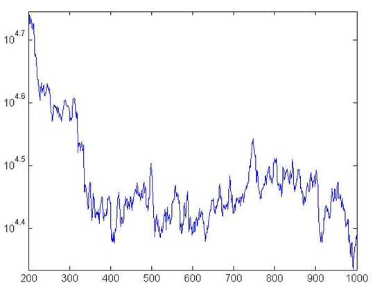
Figure 1. Production in the BS 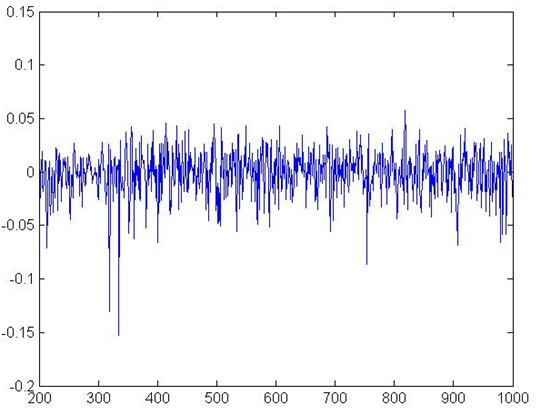
Figure 2. Aggregate Growth Rates in BS 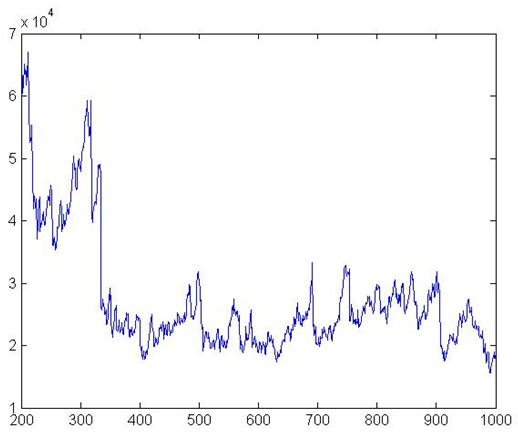
Figure 3. Total Amount of Credits 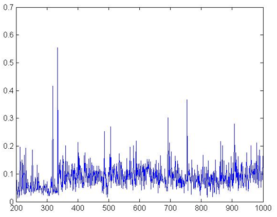
Figure 4. NPL Ratio 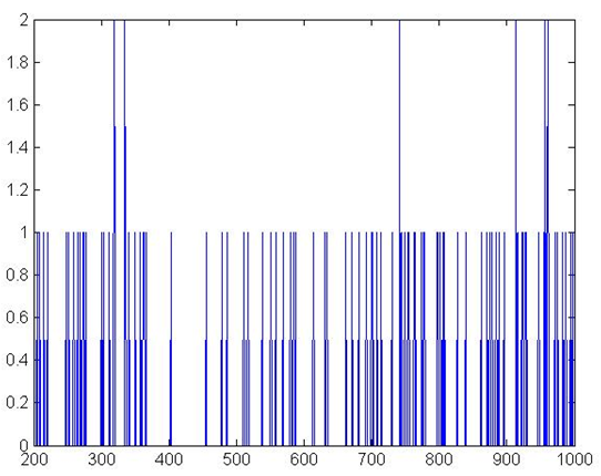
Figure 5. Banks defaults 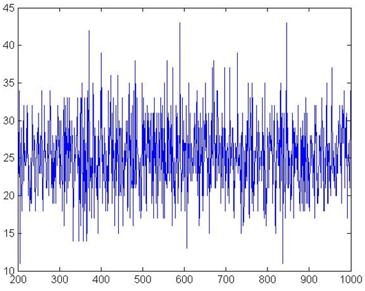
Figure 6. Firms Defaults 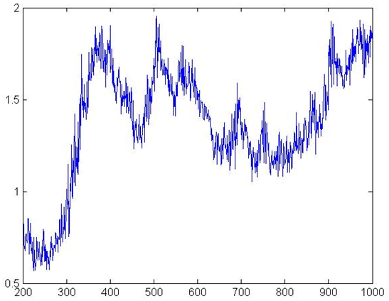
Figure 7. Firms' Leverage 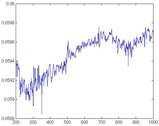
Figure 8. Interest Rates Robustness check
- 3.10
- We performed a Monte-Carlo experiment to assess the
robustness of our results. We run 100 simulations with different seeds.
The experiment shows that the results of the base model are robust, and
do not show high volatility among simulations. Indeed, mean values of
parameters do not show high standard deviations, as shown in the
selected list of statistic in Table 2[8]. The net-work based
financial accelerator dynamic recurs in all the simulations. Both kinds
of bankruptcies can be observed in the simulations. No credit
asymmetries were observed either in base simulation or in robustness
tests. This means there is no situation in which banks offer credit but
firms do not demand it.
Table 2: Robustness check, selected statistics min mean max std. dev. Growth mean % 0.08 0.10 0.12 0.01 Growth std. dev. % 2.02 2.18 2.32 0.06 Interest rate mean % 5.95 5.97 5.98 0.01 Interest rate max % 6.08 6.09 6.09 0.002 Firm defaults mean % 4.93 4.99 5.07 0.02 Bank defaults mean % 0.79 1.03 1.45 0.14 Leverage mean 0.08 1.25 1.43 0.14 Bad debt ratio mean % 7.69 8.34 8.86 0.23 Sensitivity Analysis
- 3.11
- It is customary in the Agent Based literature to perform a sensitivity analysis in order to assess the extent to which results depend on specific parameter values (see Fagiolo et al. 2007). Accordingly we re-ran the model changing one parameter each time, while keeping all the others stable. Here below we present a selection of the most significant findings.
- 3.12
- \(\varphi\) and \(\beta\): respectively the multiplier and the exponential parameter in the production function (equation 2). We increased \(\varphi\) from 2 to 4 with steps of 0.2 and \(\beta\) from 0.6 to 0.8 with steps of 0.02. Clearly, the two experiments have a very similar outcome, with the only difference being exponential changes with increasing \(\beta\). The results are very interesting in light of our analysis. When banks' only concern is capital adequacy ratio, as in our baseline scenario, an increase in productivity has positive effects on the economy also in terms of financial stability. Indeed we witness increasing growth, while mean values of bank and firm defaults, interest rate and leverage, all decrease. There is also an increase in volatility as the standard deviation of interest rates and leverage increase significantly.
- 3.13
- \(\Delta l_{max}\): maximum percentage change in a firm's leverage, relative to previous period. We change the value of \(\Delta l_{max}\) from 0.02 to 0.22 with steps of 0.02. Impacts on growth variable are limited. As expected, volatility and financial instability increase. Kurtosis, minimum, mean, and maximum levels of growth stay at almost the same level, whereas non-performing loans, bank defaults, and firm default rate increase significantly. Average interest rate rises from 5.86%, to 6.01%, while standard deviation of interest rate declines gradually.
- 3.14
- \(rmin\): policy rate and bottom level for bank interest rate. Standard deviation of growth decreases and then (with \(rmin \geq 0.05\)) follows a steady trend; mean growth increases with values of \(rmin\) between 0.05 and 0.1, because these values are more compatible with banks costs. Nonperforming loans, bank defaults, and firm defaults all decrease steadily.
- 3.15
- \(\gamma\): is the parameter of the bank specific component, related to capital adequacy ratio, of the interest rate equation (11.a). We increased \(\gamma\) from 0.005 to 0.05 by intervals of 0.005. Increasing \(\gamma\), bad debt, bank defaults, and total debt increase, while firm default rates and mean growth (with \(\gamma \geq 0.01\)) show no significant difference.
- 3.16
- \(\alpha\): the parameter used in the firm specific part of interest rate. We increased \(\alpha\) from 0.005 to 0.05 by intervals of 0.005. With higher values of \(\alpha\), the standard deviation of growth decreases steadily, while mean growth stays almost at the same level. Total debt and bank defaults decrease sharply, while firm defaults are not affected.
- 3.17
- \(CAR^\ast\): capital adequacy ratio. We run simulation with CAR ranging from 0.04 to 0.22 increasing by 0.02. It is noteworthy to see that as \(CAR^\ast\) increases, average growth rate decreases and standard deviation of growth first increases and then decreases. On the other hand, bank defaults and leverage decrease significantly, while interest rates and firm defaults decrease gradually. As expected, increasing \(CAR^\ast\) stabilizes the economy while decreasing mean growth rate.
Alternative Scenarios
- 4.1
- We devote this section to the analysis of the outcome of
different bank behaviors. Two alternative scenarios are implemented; in
the first, banks implement an aggressive competitive strategy in order
to increase their market share. In the second, we reproduced the
pro-cyclical behavior of banks.
Market Share Pricing (MSP)
- 4.2
- We tested the scenarios in which banks prioritize
increasing their market share when pricing credits. In this setting, a
bank with lower market share sets lower interest rates to attract more
clients. So, the interest rate equation 11 becomes \(f_1(MS) = \gamma
MS^\gamma\). Results are shown in table 3
and are in line with our expectations.
Table 3: Results with Market Share Pricing Mechanism (MSP) Minimum Mean Maximum Std. Dev. Bad Debt Ratio % 0.00 8.60 43.72 3.74 Bank Defaults % 0.00 3.22 22.00 2.94 Bank Net Worth 3742.90 41225.72 77623.50 19509.42 Total Debt 5250.66 21152.52 38959.30 4028.85 Firm Defaults % 0.00 5.35 9.20 1.05 Firm Net Worth 5822.35 26959.19 50379.40 8598.55 Aggregate Production 12425.90 25651.27 31484.20 2395.69 Interest Rate % 5.60 5.82 5.86 0.03 Leverage 0.73 1.41 2.22 0.30 Growth % -10.69 0.08 11.46 2.19 - 4.3
- As expected, interest rate decreases sharply. The minimum,
mean and maximum values of interest rates are below the respective
figure in the baseline scenario and short term fluctuations rise
significantly (see (Fig. 9).
Aggregate output, and average growth are lower, while non-performing
loans increase. Bank percentage is considerably higher: 1.03% in base
model and 3.22% in market share pricing mechanism. One cause of this is
that low interest rates set by banks with low market share weakens
their financial position. As expected, mean and maximum values for bank
net worth and total debt are less than (or close to the minimum
levels), the minimum values of the base model. Another noteworthy
result is that average ratio of firm defaults is above even the maximum
of average firm defaults in the robustness check tests of the base
model. Parallel to this, average and maximum values of firms' net worth
in the market-share pricing scenario are below the minimum values of
the base model. This simulation shows that when banks prioritize their
market shares in pricing, financial instability increases while there
is no significant effect on growth.
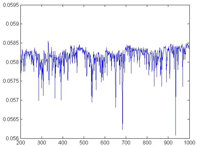
Figure 9. Interest Rates MSP 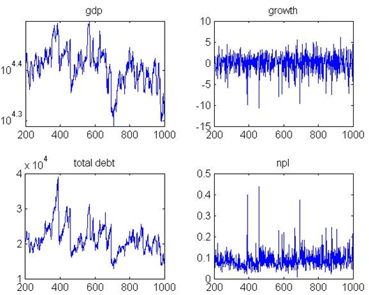
Figure 10. Output, growth, debt, and bad debt MSP 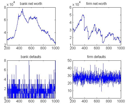
Figure 11. Banks, and firms net worth, and defaults Pro-cyclical (PC)
- 4.4
- To test effects of the pro-cyclical behavior of banks we
changed interest rate equation so that banks lower interest rate when
economy grows and vice versa (see equation 11.b).
Table 4: Results with pro-cyclical (PC) Minimum Mean Maximum Std. Dev. Bad Debt Ratio % 0.00 9.62 44.11 3.88 Bank Defaults % 0.00 4.96 24.00 4.32 Bank Net Worth 1705.70 11528.51 40106.90 11081.87 Total Debt 5262.46 17846.98 32345.10 3290.88 Firm Defaults % 0.00 5.48 10.00 1.09 Firm Net Worth 68.18 20273.42 41433.80 6646.01 Aggregate Production 12435.90 23093.32 30243.10 2179.18 Interest Rate % 4.87 6.03 6.73 0.17 Leverage 0.86 1.59 2.34 0.31 Growth % -10.72 0.07 15.13 2.23 - 4.5
- Results are univocal and show that this behavior has
detrimental effects on the economy, both in terms of production level
and financial stability. Indeed, mean growth rate falls (from 0.1%, to
0.07%). Firm defaults rise from 4.99% to 5.48%, with standard deviation
increasing from 0.02% to 1.09%. Similarly, bank defaults increase from
1.03% to 4.96%. These results show that when banks set interest rate
based on past output, which is a common real life practice, both
economic and financial instability increase.
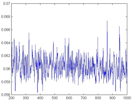
Figure 12. Interest Rates PC 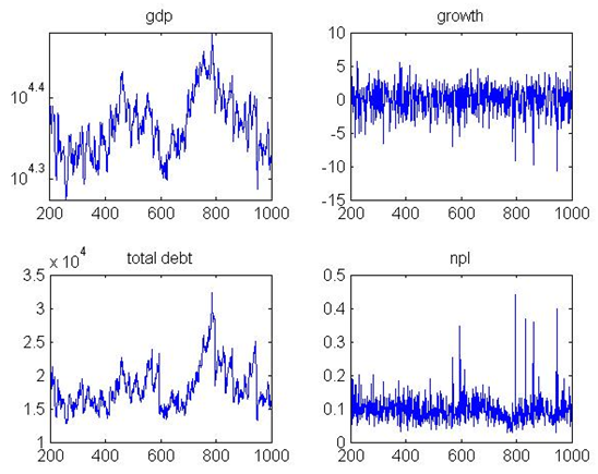
Figure 13. Output, growth, debt, and bad debt PC 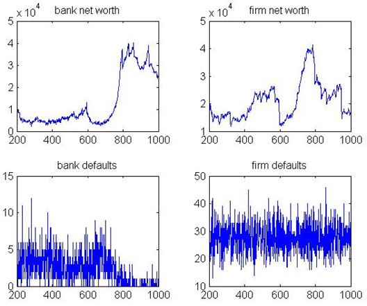
Figure 14. Bank, and firm net worth, and defaults - 4.6
- We also performed analysis of this scenario by varying values of \(\rho\) from 0.04 to 0.2 in intervals of 0.02. The aim was to assess the changes in results when banks attribute various weights to past economic performance. This exercise clearly shows that the more banks rely on recent past economic growth data to determine their interest rate, the more volatile the economy becomes, and the more the economy becomes unstable.
Conclusion
- 5.1
- In this paper we present an Agent Based model built on Riccetti et al. (2013), to analyze the potentially destabilizing role of banks as described by the Financial Instability Hypothesis (Minsky 1986). We focused on the determination of interest rates by banks and we reproduced different strategies. In the base line scenario, banks focus on the capital adequacy ratio, whereas in the two alternative scenarios they take into account their market share and recent economic growth. Minsky's analysis appears to be confirmed by our model. Changes in banks' credit pricing strategies may have noteworthy effects, and indeed, increase instability. As banks behave prioritizing market share with respect to financial soundness, non-performing loans and defaults, both in the firms and in banking sector, increase. This is in line with the network-based financial accelerator dynamic (Greenwald & Stiglitz 2003; Delli Gatti et al. 2010a). Similarly when banks calibrate their credit pricing according to the observed growth rate, both economic and financial instability increase. Other results show how different strategies may contribute to enhance the stability of the system. Financial stability increases when banks support firms in need of liquidity and if they raise their capital adequacy ratio requirements. Our model is the first Agent Based model focusing on banks destabilizing credit-pricing strategy, therefore it can be enlarged in multiple directions. For example, a more detailed analysis of balance sheets interrelation between different firms and banks could provide for a clearer depiction of the evolution of crisis, and of the financial accelerator. Furthermore including a households sector, as well as endogenous price, could allow to have a more realistic productive sector and therefore to have a better understanding of the links between the real and the financial side of the economy. Other developments could refer to customer loyalty and the entrance of new units after bankruptcies.
Notes
-
1The
word mainstream is here used with respect to macroeconomics, referring
to the Dynamic Stochastic General Equilibrium (DSGE) models (Blanchard 2008;
Woodford
2009), and with respect to financial economics, referring the
Efficient
Market Hypothesis (Fama 1991).
On the need for alternatives see also Trichet (2010).
2'They actively solicit borrowing customers, undertake financing commitments, build connections with business and other bankers, and seek out funds' (Minsky 1986, pp.256–257).
3This over-simplified economy was defined by Minsky "basic skeletal capitalist economy" (1986, p. 250 ) as the financing of business activity is at the core of his analysis.
4We relied on a balance sheet approach to build our model because we believe that balance sheets and cash flows are fundamental in understanding the links among agents in the firm-bank linkages in a network theoretical framework.
5Simulation program is written in C++ language. Interested reader can find the code of the base model at the link: https://www.openabm.org/model/4739/version/1/view
6This is coherent with our model, as market share can be considered as a proxy for the size of transactions and market structure, while economic growth expectations can be considered a proxy for variance of interest rates.
7For example for a comparison with the empirical evidence in the European Union see ECB (2014).
8For the complete list of 15 statistics please contact the authors
Appendix
-
Parameters Value
Table 5: Initial parameters of the base model Parameter Value Explanation \(\varphi\) 3 production function of the firm \(\beta\) 0.7 production function of the firm \(\Delta l_{max}\) 0.1 target leverage setting function \(u\) 0.1 expected gross profit \(\sigma^2\) 0.01 variance of random variable in profit function \(\theta\) 0.5 ratio of total capital that can be liquidized \(lqlim\) 0.4 level of relative liquidity for liquidity bankruptcy \(rmin\) 0.02 interest rate floor \(\gamma\) 0.02 interest rate setting, bank parameter \(\alpha\) 0.02 interest rate setting, firm parameter \(RR\) 0.5 recovery rate in case of default \(c\) 0.005 bank operational costs \(CAR^\ast\) 0.12 minimum legal capital adequacy ratio \(MB\) 15 maximum number of banks that a firm can work \(N\) 2 number of banks other than current banks, firms ask credit \(\lambda\) 0.4 exponential distribution parameter for credit term \(H\) 4 maximum number of credit terms \(A_i\) 10 Initial net worth of a firm \(A_z\) 20 Initial net worth of a bank Table 6: Robustness Check Results min mean max std. dev. Bad debt ratio mean % 7.69 8.34 8.86 0.23 Bad debt ratio max % 29.84 44.41 72.35 9.37 Bad debt ratio std. dev. % 3.67 4.06 4.51 0.18 Bank defaults mean % 0.79 1.03 1.45 0.14 Bank defaults max % 16 25.18 36.00 4.58 Bank defaults std. dev. % 2.11 2.52 2.90 0.17 Bank net worth mean 49954.74 86255.04 144326.33 19025.01 Bank net worth max 79587.80 176827.15 378882.00 56649.14 Bank net worth std. dev. 20588.03 44475.33 103964.61 15638.91 Total debt min 5233.99 5250.44 5263.53 6.28 Total debt mean 24882.44 27326.41 31300.94 1387.93 Total debt max 37865.50 55817.71 97673.60 10862.90 Total debt std. dev. 4624.98 8188.75 15920.61 2273.61 Firm defaults mean % 4.93 4.99 5.07 0.02 Firm defaults max % 7.80 8.58 9.60 0.38 Firm defaults std. dev. % 0.99 1.04 1.08 0.02 Firm net worth min 5799.13 5930.19 6051.88 56.06 Firm net worth mean 30898.55 39736.76 57704.58 5380.13 Firm net worth max 55070.20 99447.87 211498.00 28572.48 Firm net worth std. dev. 8614.76 21586.64 53546.45 8266.49 Aggregate production min 12411.80 12425.75 12436.90 5.33 Aggregate production mean 28868.08 31044.20 34266.52 1133.60 Aggregate production max 38204.30 48283.84 65440.70 5682.50 Aggregate production std. dev. 3209.67 6058.20 11165.52 1725.48 Interest rate min % 5.86 5.91 5.95 0.02 Interest rate mean % 5.95 5.97 5.98 0.01 Interest rate max % 6.08 6.09 6.09 0.002 Interest rate std. dev. % 0.03 0.03 0.04 0.003 Leverage min 0.00 0.61 0.96 0.13 Leverage mean 0.08 1.25 1.43 0.14 Leverage max 0.33 2.18 2.35 0.19 Leverage std. dev. 0.19 0.32 0.44 0.05 Growth min % -22.38 -12.35 -7.84 2.94 Growth mean % 0.08 0.10 0.12 0.01 Growth max % 11.21 13.09 14.78 0.72 Growth std. dev. % 2.02 2.18 2.32 0.06
References
- ADRIAN, T., Colla, P., &
Shin, H.S., (2012). Which financial frictions? Parsing the evidence
from the financial crisis of 2007–9. NBER Working Papers 18335
BATTISTON, S., Delli Gatti, D., Gallegati, M., Greenwald, B., & Stiglitz, J.E., (2007). Credit chains and bankruptcies avalanches in supply networks. Journal of Economic Dynamics and Control 31 (6), 2061–2084.
BATTISTON, S., Delli Gatti, D., Gallegati, M., Greenwald, B., & Stiglitz, J.E. (2012). Default cascades: When does risk diversification increase stability?, Journal of Financial Stability, 8(3), 138–149
BERNANKE, B., & Blinder, A. (1988). Credit, money, and aggregate demand, The American Economic Review, 435–439
BERNANKE, B., & Blinder, A. (1992). The federal funds rate and the channels of monetary transmission, The American Economic Review, 901–921
BERNANKE, B., & Gertler, M. (1989). Agency costs, net worth and business fluctuations, American Economic Review, (79), 14–31
BERNANKE, B., & Gertler, M. (1990). Financial fragility and economic performance, The Quarterly Journal of Economics, 105, 87–114
BERNANKE, B., Gertler, M., & Gilchrist, S. (1996). The financial accelerator and the flight to quality, The Review of Economics and Statistics, 78(1), 1–15
BLANCHARD, O. (2008) The state of macro, NBER Working Paper No. 14259.
BROCK, W.A., & Hommes, C.H. (1998). Heterogeneous beliefs and routes to chaos in a simple asset pricing, Journal of Economic Dynamics and Control, 22(8–9), 1235–1274.
CHINAZZI, M., & Fagiolo, G. (2013). Systemic risk, contagion and financial networks: A survey. LEM Papers Series 2013/08. Pisa: Sant'Anna School of Advanced Studies.
DELLI GATTI, D., Gaffeo, E., Gallegati, M., Giulioni, G., Kirman, A., Palestrini, A., & Russo, A. (2007). Complex dynamics and empirical evidence, Information Sciences, (177), 1204–1221
DELLI GATTI, D., Gallegati, M., Greenwald, B., Russo, A., & Stiglitz, J.E., (2009). Business fluctuations and bankruptcy avalanches in an evolving network economy. Journal of Economic Interaction and Coordination 4 (2), 195–212.
DELLI GATTI, D., Gallegati, M., Greenwald, B.C., Russo, A., & Stiglitz, J.E. (2010a). The financial accelerator in an evolving credit network, Journal of Economic Dynamics and Control.
DELLI GATTI, D., Gaffeo, E. & Gallegati, M. (2010b). Complex Agent-Based Macroeconomics: a Manifesto for a New Paradigm. Journal of Economic Interaction and Coordination, 5(2), 111–135.
ECB (2014). Banking Structures Report – October 2014, European Central Bank.
FAGIOLO, G., Moneta, A., & Windrum, P. (2007). A critical guide to empirical validation of agent-based models in economics: Methodologies, procedures, and open problems, Computational Economics, 30(3), 195–226
FAMA, E. F. (1991). Efficient capital markets: II, The Journal of Finance 46 (5), 1575–1617
FARMER, J.D., & Foley, D. (2009). The economy needs agent-based modelling, Nature, (460), 685–686
FLANNERY, M.J., & Rangan, K.P. (2006). Partial adjustment toward target capital structures. Journal of Financial Economics, 79(, (3), 469-506.
FRANK, M.Z., & GOYAL V.K., (2008). Trade-off and pecking order theories of debt. Handbook of Corporate Finance: Empirical Corporate Finance, Vol. 2, Handbook of Finance Series, Chapter 12, Elsevier/North-Holland, Amsterdam.
GABAIX, X. (2011). The granular origins of aggregate fluctuations, Econometrica, 79(3), 733–772
GABBI, G., Iori, G., Jafarey, S., & Porter, J., (2015). Financial regulations and bank credit to the real economy, Journal of Economic Dynamics and Control, 50(C), 117–143.
GALLEGATI, M., Giulioni, G., & Kichiji, N. (2003). Complex dynamics and financial fragility in an agent based model, Advances in Complex Systems, 6(3) [doi:10.1142/S0219525903000888]
GALLEGATI, M., Palestrini, A., & Rosser, J.B., (2011). The Period Of Financial Distress In Speculative Markets: Interacting Heterogeneous Agents And Financial Constraints, Macroeconomic Dynamics, Cambridge University Press, vol. 15(01), pp. 60–79, February.
GALLEGATI, M., Giulioni, G., & Kichiji, G. (2003). Complex dynamics and financial fragility in an agent-based model, Advances in Complex Systems 6 (2003) 267–282. [doi:10.1142/S0219525903000888]
GAMBACORTA, L. (2004). How do banks set interest rates?, NBER Working Series, 10295
GREENWALD, B.C., & Stiglitz, J.E. (1993). Financial market imperfections and business cycles, The Quarterly Journal of Economics, 108(1), 77–114 [doi:10.2307/2118496]
GRILLI, R., Tedeschi, G. & Gallegati, M. (2014). Bank interlinkages and macroeconomic stability, International Review of Economics & Finance, 34(C), 72–88. [doi:10.1016/j.iref.2014.07.002]
HO, T.S.Y., & Saunders, A. (1981). The determinants of bank interest margins: Theory and empirical evidence, Journal of Financial and Quantitative Analysis, 16(04), 581–600 [doi:10.2307/2330377]
KIRMAN, (1993). Ants, rationality, and recruitment. Quarterly Journal of Economics, 108(1), 137-156 [doi:10.2307/2118498]
HOVAKIMIAN, A., Opler, T., Titman, S., (2006). The debt-equity choice. Journal of Financial and Quantitative Analysis, 36, 1-24 LAVOIE, M. & Seccareccia, M, (2001). Minsky's Financial Fragility Hypothesis_ A Missing Macroeconomic Link? in Ferri, P. and Bellofiore, R. (Eds) Fragility and Investment in the Capitalist Economy: The Economic Legacy of Hyman Minsky, Volume II. Cheltenham: Edward Elgar.
LUX, T. (1995). Herd Behaviour, bubbles and crashes. he Economic Journal, 105, 881-896 [doi:10.2307/2235156]
MAUDOS, J., & Guevara J.F. (2004). Factors explaining the interest margin in the banking sectors of the European Union, Journal of Banking & Finance, 28(9), 2259–2281 [doi:10.1016/j.jbankfin.2003.09.004]
MINSKY, H.P. (1976). John Maynard Keynes, London: Macmillan.
MINSKY, H.P. (1986). Stabilizing an Unstable Economy, New Haven: Yale University Press, 1986.
MINSKY, H.P, (1992). The Financial Instability Hypothesis, Working Paper No. 74, The Levy Economics Institute, May.
RECCHIONI, M.C., Tedeschi, G., & Berardi, S. (2014). Bank's strategies during the financial crisis, FinMaP-Working Paper, No. 25, 2014
RICCETTI, L., Russo, A., & Gallegati M. (2013). Leveraged network based financial accelerator, Journal of Economic Dynamics & Control 37 (2013) 1626–1640. [doi:10.1016/j.jedc.2013.02.008]
SAUNDERS, A., & Schumacher, L. (2000). The determinants of bank interest rate margins: an internal study, Journal of International Money and Finance, 19(6), 813–832. [doi:10.1016/S0261-5606(00)00033-4]
STIGLITZ, J.E. & Greenwald, B. (2003). Towards a new paradigm in monetary economics, Cambridge University Press. [doi:10.1017/CBO9780511615207]
TESFATSION, L., & Judd, K.L. (2006). Handbook of Computational Economics, Volume 2: Agent Based Computational Economics, North Holland.
TRICHET, J. C. (2010). Reflections on the nature of monetary policy non-standard measures and finance theory. Speech by Jean-Claude Trichet, President of the ECB, Opening address at the ECB Central Banking Conference Frankfurt, 18 November 2010. http://www.ecb.europa.eu/press/key/date/2010/html/sp101118.en.html
WOODFORD, M. (2009). Convergence in Macroeconomics: Elements of the New Synthesis.American Economic Journal: Macroeconomics, 1(1), 267-79. [doi:10.1257/mac.1.1.267]