
 Abstract
- Human mate choice is a boundedly rational process where individuals search for their mates without appealing to optimization techniques due to informational, computational and time constraints. A seminal work by Todd and Miller (1999) models this search process using simple heuristics, i.e. decision rules that adjust individuals' aspiration levels adaptively. To identify the best heuristic among a number of alternatives, they consider fixed measures of success. In this paper, we deal with the same identification problem by examining whether these heuristics would be favored by behavioral selection. To this aim, we extend the two-phase search model of Todd and Miller (1999) to a behavioral (strategic-form) game in which each individual in the population is a distinct player, each player's strategy space contains the same four heuristics (adjustment rules), and the payoff of each player is measured by the likelihood of his/her mating. For this game, we ask whether any strategy profile at which the whole population plays the same heuristic can be behaviorally stable with respect to the Nash equilibrium concept. Our simulations show that the unanimous use of the Take the Next Best Rule by the whole population never becomes an equilibrium in the simulation range of adolescence lengths. While the Adjust Relative Rule is found to be behaviorally stable for a wide part of the simulation range, especially for medium to high adolescence lengths, the rules Adjust Up/Down and Adjust Relative/2 are favored by behavioral selection for a small part of the simulation range and only when the adolescence is long and short, respectively. We make the final evaluation of the four heuristics with respect to a new success measure that integrates a behavioral stability metric proposed in this paper with two metrics of Todd and Miller (1999), namely the likelihood and the assortativeness of the mating generated by the heuristic in use.
- Keywords:
- Mate Choice, Mate Search, Simple Heuristics, Agent-Based Simulation, Behavioral Stability, Equilibrium Strategies
Introduction
- 1.1
- A strand of literature in cognitive psychology, pioneered by Todd and Miller (1999), studies the dynamics underlying the human mate choice using boundedly rational models. These models are based on the assumption that due to computational, informational and time constraints, individuals do not optimize (either unboundedly or under constraints) in choosing their mates, but instead they use some decision heuristics (Gigerenzer, Todd & the ABC Research Group 1999). These heuristics derive from the Simon's (1955) earlier concept of `satisficing' by means of aspiration levels, which individuals are assumed to form by interacting with a number of dates sequentially before the actual mate search takes place. A heuristic such formed is satisficing in the sense that any pair of individuals interacting in the search phase are mated when their aspirations are mutually met.
- 1.2
- The practical applicability of these new models of mate search were investigated by recent studies, including Hills and Todd (2008), Todd et al. (2005) and Simão and Todd (2003), which showed that simple heuristics can generate both robust and realistic demographic patterns. However, an important question still remains: Which decision heuristics are more likely to be adopted by a mating population? On the empirical side, the data from speed-dating has recently enabled Beckage et al. (2009) to deal with this question. Their results, while confirming that individuals adjust their aspiration levels in response to experience during the speed-dating session, were inconclusive to select the best one among various aspiration-adjusting models. On the normative side, the same question was originally tackled by Todd and Miller (1999) themselves, who attempted to evaluate the heuristics they proposed by comparing their produced likelihood of mating. Since this particular metric turned out to be inadequate for the perfect differentiation of alternative heuristics, they considered additional success measures. One such measure is the degree of assortative mating produced, i.e., the degree of similarity of mated pairs. Obviously, the restriction to this particular measure can be rationalized by the fact that the degree of assortativeness is a good indicator of the stability (survival) of the mating outcome. Yet, this does not alleviate a disturbing fact that this metric, as a subjective choice of an outside analyst observing the mating problem in question, is not necessarily internalized by the individuals in the mating population. In other words, "the degree of assortative mating … is not necessarily something that would be optimized by selection" (Fawcett et al. 2012, p. 7).
- 1.3
- The need for taking the forces/mechanisms of evolutionary or behavioral selection into consideration to properly assess alternative heuristics in mate search should be very clear, once we notice that the human mate choice is not only a search-theoretical decision problem but also a noncooperative game-theoretical problem (or a behavioral game) where the mating likelihood of each individual is affected by the strategies or actions of (decision heuristics followed by) all individuals in the population. Evolutionary game theory (Maynard Smith 1982) posits that solutions of such games have to be evolutionarily stable in the sense that natural selection yields a stable (equilibrium) state at which no alternative strategies can spread and invade within the mating population. However, for the problem of human mating it would be more reasonable to assume that a change in the frequencies of the strategies played by the population occurs not due to natural selection but because of the capability and willingness of individuals to adjust their strategies according to the conditions of the game they are playing. In such problems, a stable frequency of strategies that is called a behaviorally stable strategy (Giraldeau and Dubois 2008; also known as developmentally stable strategy, Dawkins 1976) is reached as a Nash (1950) equilibrium, where no individual has any incentive to unilaterally change his/her behavior (strategy). Using this behavioral notion of stability, we are ready to formulate the main question in this paper: Can the mating population's unanimous use of a mate search heuristic be a stable situation in behaviorally stable (Nash equilibrium) strategies? To answer this question we will extend the two-sided mate choice model of Todd and Miller (1999) to a behavioral (strategic-form) game, where the set of players involves all individuals in the mating population, the strategy space of each player contains the same four heuristics (to be discussed below) and the payoff of each player at each strategy profile is measured by his/her likelihood of mating.
- 1.4
- Examination of the behavioral stability of simple heuristics in the two-sided mate search is novel to this study; however, the problem of finding stable outcomes in two-sided marriage markets dates back to Gale and Shapley (1962). The focus of their study was to show the general existence of stable matings where there exist no two individuals of opposite sexes who are not a pair but prefer each other to their current partners and no individual who is matched but prefer being single to his/her partner. Importantly, this early work offered an iterative procedure, called the deferred acceptance algorithm, by which one can find a stable matching in every population of males and females. This algorithm, which was independently discovered by the National Residency Matching Program (NRMP) in the United States (US) and had been used since 1950s in matching medical interns with hospital residency positions (as shown by Roth 1984), gained its popularity especially with its use to match students with public high schools in New York City and Boston.[1]
- 1.5
- Apparently, the two-sided stable matching model of Gale and Shapley (1962) has led to the emergence of a large literature in economic theory and applied mechanism design. Despite that, the amount of research studying the formation of marriages in human societies is extremely little.[2] One reason is that in marriage environments, unlike in school choice or hospital-intern problems, there exists no central agency applying a particular mating algorithm. Besides, individuals have no information about potential mates before the actual mating takes place. Given these constraints, it has become inevitable to study the formation of marriages using `decentralized' and `sequential' models of mate search, where individuals gain, by sequentially encountering some potential mates, all relevant information on which they base their final mating decisions.[3] Relatedly, a strand of literature (Dombrovsky and Perrin 1994; Mazalov et al. 1996; Todd and Miller 1999; Collins et al. 2006) conditioned the information for mating decisions on the self mate values of individuals, also assuming that individuals do not completely know but can partially learn (or approximate) their self mate values by using feedbacks from potential mates they interact before they are mated. Among this literature, the paper of Todd and Miller (1999) was the first to consider a mate-choice model with two-sided (mutual) search strategies. Basically, the model consists of two consecutive phases. Individuals first go through an `adolescence' (learning) phase in which they randomly interact (date) with a number of individuals of the opposite sex and possibly exchange information with their dates. After each interaction each individual adjusts his/her aspiration level (as a proxy of his/her self mate value) according to a particular adjustment rule used by the whole population.[4] All individuals next proceed to a `mating' phase where they randomly interact with potential mates and decide whom to make a proposal for mating. In this phase, each pair of individuals in the mating pool are considered to be successful and removed from the pool as mated if they simultaneously make proposals to each other. This phase ends after a stage at which either the mating pool becomes empty or each individual in the mating pool has already been paired unsuccessfully with all available individuals of the opposite sex.
- 1.6
- The adjustment rules (heuristics) considered by Todd and Miller (1999) in the adolescence phase of their model involve Take the Next Best, Adjust Up/Down, Adjust Relative, and Adjust Relative/2.[5] According to the Take the Next Best Rule, individuals start the adolescence period with an initial aspiration level of zero, and at each instance of dating each individual sets his/her aspiration to the mate value of his/her date if that value is above his/her current aspiration level. Thus, individuals leave the adolescence phase with an aspiration level set to the highest mate value they have observed.
- 1.7
- The remaining three adjustment rules set the initial aspiration level of each individual to the average mate value of all individuals of the same sex. These rules also require that each individual exchanges information with his/her date as to whether they have found each other desirable; i.e., the observed mate value of the date is above one's aspiration level. According to the Adjust Up/Down Rule, each individual adjusts, at each instance of dating, his/her aspiration upwards by a constant shift parameter if he/she learns that the date finds him/her desirable, and adjusts his/her aspiration downwards by the same parameter otherwise. The Adjust Relative Rule differs from the previous rule in that if the date's mate value is above the current aspiration level of an individual and the date still finds this individual desirable, the individual raises his/her aspiration level. Conversely, if the date's mate value is below the current aspiration level of an individual and the date does not find this individual desirable, the individual reduces his/her aspiration level. In other possible cases, individuals do not make any adjustments. In Adjust Up/Down Rule and Adjust Relative Rule, the adjustment parameter is constant during the adolescence phase and inversely related to the length of this phase (i.e., the common number of dates interacted by each individual). Finally, the Adjust Relative/2 Rule differs from Adjust Relative in the adjustment parameter, which is no longer constant during the adolescence phase but is dependent on the difference between the aspiration level of each individual and the mate value of his/her date.
- 1.8
- Computer simulations of Todd and Miller (1999) show that among the four adjustment rules the Take the Next Best Rule yields the lowest number of matings. On the other hand, the highest number of matings are generated by the Adjust Relative/2 Rule when adolescence length is short to medium, and by the Adjust Up/Down and Adjust Relative Rules when adolescence is longer. Since in terms of the likelihood of mating no adjustment rule dominates every other rule for all adolescence lengths, Todd and Miller (1999) considered additional measures of `population-level mating success' to identify the best adjustment rule. One such measure is the mean mate value of all mated individuals', with middle values indicating more successful mate search strategies. Another measure they consider is the mean within-pair difference in mate value, with lower values indicating strategies that are more successful. Todd and Miller (1999) show that of the three rules that all dominate the Take the Next Best Rule in terms of the likelihood of mating, Adjust Relative/2 has the best performance in terms of these additional measures of success for a great part of adolescence lengths.
Table 1: The adjustment rules (asp = aspiration; n = # of individuals in each sex; S = length of adolescence; V = the maximal mate value.) Conditions Take the Next Best Adjust Up/Down Adjust Relative Adjust Relative/2 The initial value of aspiration is given to individual i aspi,0= 0 aspi,0= V/2 aspi,0= V/2 aspi,0= V/2 Individual i finds the date in stage s desirable aspi,s = mate_value_date_s Individual i finds the date in stage s nondesirable aspi,s = aspi,s-1 The date in stage s finds individual i desirable aspi,s = aspi,s-1 + δ
δ = (V/2)/(1+S)The date in stage s finds individual i nondesirable aspi,s = aspi,s-1 − δ
δ = (V/2)/(1+S)Individual i and the date in stage s find each other desirable aspi,s = aspi,s-1 + δ
δ = (V/2) / (1+S)aspi,s = aspi,s-1 + δ(i,s)
δ(i,s) = |mate_value_date_s- aspi,s-1| / 2Individual i and the date in stage s find each other nondesirable aspi,s = aspi,s-1 − δ
δ = (V/2) / (1+S)aspi,s = aspi,s-1 − δ(i,s)
δ(i,s) =|mate_value_date_s- aspi,s-1|/ 2Either individual i or the date in stage s finds the other desirable aspi,s = aspi,s-1 aspi,s = aspi,s-1 - 1.9
- Clearly, the (ex-post) instability of some matings is inevitable in environments where matings are decentralized, individuals have incomplete information about potential mates and the search is not exhaustive. The mean difference between the mate values of partners, as a measure of mating success, can provide some indirect information about the stability of the mated pairs formed under a particular adjustment rule.[6] As already argued by Todd and Miller (1999), with higher values of this measure an adjustment rule may lead to less stable matings, since mated pairs with diverse mate values are more prone to the danger of partner switching in a dynamic framework. Recently, Eriksson and Hägsström (2008) dealt with directly estimating the degree of instability that one can expect in decentralized mating environments. Using the proportion of blocking pairs among all possible pairs as a measure of instability, they showed that in environments where all individuals use a particular heuristic with a threshold lowered gradually over the mate search (as in Simão and Todd 2002), the expected instability of matings tends to zero as the number of agents grows if individuals' preferences are random and independent. Following up this work, Eriksson and Strimling (2009) show with the help of experimental data how the total search effort and the expected instability of the mating outcome vary with various other preference structures.
- 1.10
- Although the main interest of this paper is to examine the behavioral (strategic) stability of the alternative heuristics in sequential mate search, the final evaluation of these heuristics is made with respect to an individual-level composite payoff function. This new success measure takes into consideration for each heuristic the resulting average likelihood of mating, the resulting average outcome stability measured by the assortativeness of the mating, as well as the intensity of the behavioral stability of the heuristic in use.
Mutual Sequential Mate Search Model
- 2.1
- We consider the mutual sequential mate search model of Todd and Miller (1999), where a population N involves a set of males, M={m1, m2, … , mn} and a set of females F={ f1, f2, … , fn }, with n > 1. Each individual i ∈ N has a (self) mate value, v(i), which is a randomly drawn from the uniformly distributed values over the interval [ 0,V ]. Mate value of each individual is always unknown to himself/herself.
- 2.2
- Mate search consists of two phases. The first phase is called `adolescence' or `learning' phase, where each individual adjusts his/her aspiration level based upon the adjustment rule he/she follows. This phase consists of S consecutive stages of dating, with S < n. (In other words, the length of adolescence is S.) At stage s ∈ {1, 2, … , S}, individual i ∈ N randomly meets a date d(i,s) of opposite sex, whose mate value v(d(i,s)) is immediately known to individual i. Individual i finds the date d(i,s) desirable at stage s if v(d(i,s)) ≥ a(i,s-1), i.e., the mate value of the date is not below his/her aspiration at the beginning of stage s. Here, it is assumed that a(i,0) is exogenously given to individual i at the beginning of stage 1. Depending on the adjustment rule, individual i and the date d(i,s) may exchange information as to whether they find each other desirable at stage s. Then, individual i forms his/her aspiration level, a(i,s), corresponding to stage s.
- 2.3
- With the aspiration level a(i,S) formed at the last stage of the adolescence phase, individual i next enters the second phase of mate search, called the `mating' phase. This phase may also have multiple stages depending on the mating outcome in the first stage. At the beginning of the first stage in the mating phase, all individuals are in the mating pool. In each stage of the mating phase, males and females in the mating pool are randomly paired to assess each other for a possible mating. If both individuals in a pair, after learning the mate values of each other, make a proposal to each other, then they are mated and removed from the mating pool. Otherwise, both individuals remain in the mating pool, as available for the next stage, if any. The mating phase ends after a finite stage at which either the mating pool becomes empty or each individual in the mating pool has already been paired with all available individuals of the opposite sex.
- 2.4
- Below, we describe four adjustment rules (taken from Todd and Miller 1999), according to which individuals can update their aspiration levels in the adolescence phase.
- 2.5
- Take the Next Best (TNB) Rule: This is a modification of the 37% rule in the "secretary problem" (Ferguson 1989; Seale and Rapoport 1997), as each individual dates with (S/n)% of the available candidate mates in the adolescence phase.[7] According to this rule, at a stage of dating s, individual i sets the corresponding aspiration level to the mate value of the date, v(d(i,s)), if individual i finds the date d(i,s) desirable, and sets it to the aspiration level corresponding to the previous stage, a(i,s-1), otherwise. Formally,
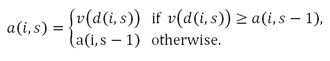
So, individual i enters the mating phase with the aspiration level a(i,S)= max{ a(i,0), v(d(i,1)), v(d(i,2)), …, v(d(i,S))}. For this rule, a(i,0) is assumed to be zero, the lowest possible mate value.
- 2.6
- For the following three adjustment rules, it is assumed that at each stage of learning each individual is informed by the date whether the date found him/her desirable. Moreover, for these adjustment rules a(i,0) is assumed to be V/2, the mean mate value of all males and of all females.
- 2.7
- Adjust Up/Down Rule: This rule is formulated as follows:
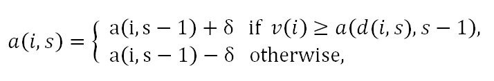
where δ=(V/2) / (1+S). Here, individual i adjusts up his/her stage s-1 aspiration a(i,s-1) by the constant δ to obtain stage s aspiration a(i,s) if the date d(i,s) finds individual i desirable. Otherwise, individual i adjusts down a(i,s-1) by δ to obtain a(i,s).
- 2.8
- Adjust Relative Rule: According to this rule, the aspiration of individual i at stage s is given by
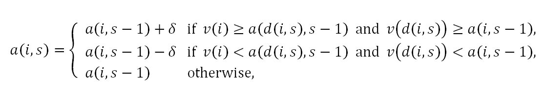
where δ=(V/2) / (1+S). Differing from the previous rule, now there is the possibility of nonadjusting in addition to up and down adjusting. Here, individual i adjusts up his/her stage s-1 aspiration a(i,s-1) by δ to obtain stage s aspiration a(i,s) if individual i and the date d(i,s) find each other desirable. If none of the dating individuals i and d(i,s) finds the other desirable, then individual i adjusts down a(i,s-1) by δ to obtain a(i,s). In other possible cases, individual i does not adjust his/her aspiration level at stage s and he/she sets a(i,s) to a(i,s-1).
- 2.9
- Adjust Relative/2 Rule: This rule differs from the Adjust Relative Rule in that the size of adjustments is neither constant over the individuals nor over the stages of adolescence. For individual i, the size of adjustment at stage s is equal to the half of the difference between the mate value of the date and the aspiration level of individual i at the end of previous stage. Thus, the rule is given by
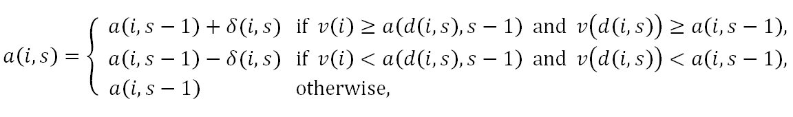
where δ(i,s)= | v(d(i,s)) - a(i,s - 1)| / 2.
- 2.10
- Using a population with n=100 (i.e., 100 males and 100 females), the maximal mate value V set to 100, and mate values uniformly distributed to individuals, Todd and Miller (1999) simulated the likelihood of mating (the number of mated pairs formed) corresponding to each adjustment rule, when the length of adolescence S is changed from 1 to 90. Considering the same mating environment, we have conducted 100 (Monte Carlo) simulations at each value of S to reproduce their findings in Figure 1. (We have used the GAUSS Software Version 3.2.34 [Aptech Systems 1998] for all simulations in this paper.)
- 2.11
- Apparently, for nearly all adolescence lengths (2 < S ≤ 90), the TNB Rule is dominated by each of the other rules in terms of the produced likelihood of mating. Figure 1 also shows two sharp findings that for short adolescence lengths (2 ≤ S ≤ 24 or 26 ≤ S ≤ 31), the Adjust Relative/2 Rule generates the highest number of matings among the four adjustment rules; whereas when adolescence is medium to long (44 ≤ S ≤ 90), the Adjust Up/Down Rule generates the highest number of matings, performing slightly better than the Adjust Relative Rule. It is also evident that both Adjust Up/Down and Adjust Relative are significantly superior to Adjust Relative/2 when adolescence is long.
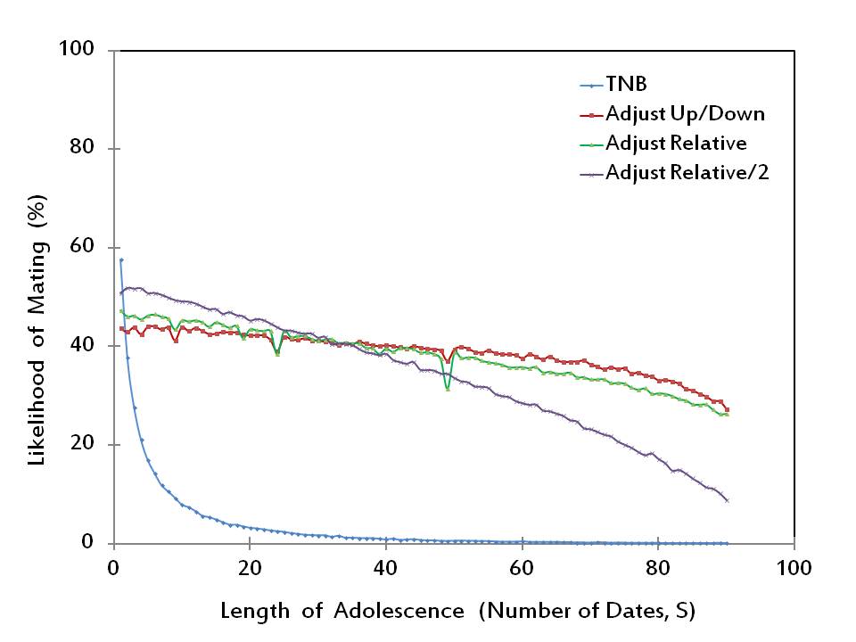
Figure 1. The likelihood of mating - 2.12
- It is clear from Figure 1 that the likelihood of mating by its own does not suffice for a complete measure of success, since no adjustment rule dominates every other rule for all adolescence lengths. An additional measure used by Todd and Miller (1999) is the mean within-pair difference in mate value. Rules that have lower scores with respect to this measure are considered more successful as they would lead to more stable matings. The performances of the four adjustment rules with respect to this second measure of success are reported in Figure 2. (Our results, which are obtained by conducting 100 simulations at each value of S, closely resemble those of Todd and Miller 1999.)
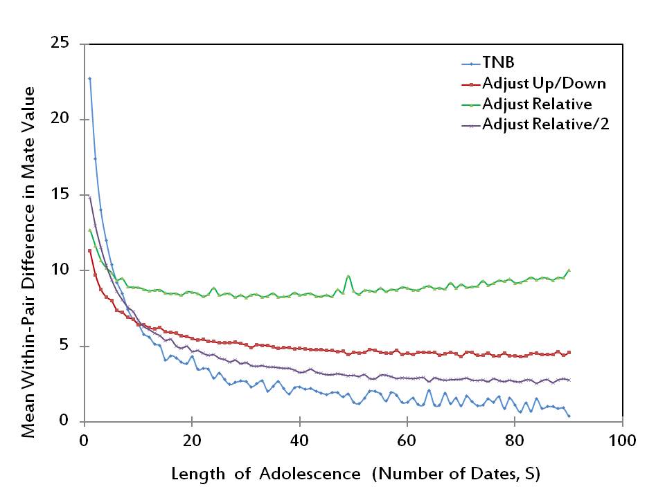
Figure 2. The mean within-pair difference in mate value - 2.13
- Figure 2 shows that overall the TNB Rule performs as the best rule with respect to this second measure of success. However, among the three adjustment rules, Adjust Up/Down, Adjust Relative and Adjust Relative/2, which cannot be ranked in terms of likelihood of mating, the lowest value of mean within-pair difference in mate value is produced by Adjust Up/Down if adolescence is very short (S ≤ 10) and by Adjust Relative/2 otherwise.
Adjustment Rules as Equilibrium Play
- 3.1
- We will now investigate whether any of the four adjustment rules described above can be favored by behavioral evolution. Specifically, we will check whether the unanimous use of a particular adjustment rule by the whole population is a Nash equilibrium of a behavioral (strategic-form) game played right before the adolescence phase. In this game, the set of players involves all individuals in the population, the strategy space of each player contains the same four adjustment rules and the payoff of each player at each strategy profile is simply his/her likelihood of mating. For a formal treatment, we introduce the following definitions.
- 3.2
- Let R ={TNB, Adjust Up/Down, Adjust Relative, Adjust Relative/2} denote the strategy space of each individual i. Let r =(rm1,…, rmn,rf1,…,rfn) ∈ R 2n denote a strategy profile of the society. In particular, we denote by rTNB the strategy profile at which each individual plays the strategy TNB, i.e. riTNB = TNB for all i ∈ N. We similarly define the strategy profiles rAUD, rAR, and rAR2 such that all individuals in the society play Adjust Up/Down under the profile rAUD, Adjust Relative under rAR, and Adjust Relative/2 under rAR2. Also, for all i ∈ N and r ∈ R 2n define the 2n-1 dimensional profile r-i such that r = (ri, r-i). For any strategy profile r ∈ R 2n, let μi(r) denote the likelihood that individual i is mated to someone of the opposite sex when he/she uses the strategy ri, while the rest of the society uses their respective strategies in r-i.
- 3.3
- We say that a strategy profile is a Nash equilibrium if there exists no individual that can increase his/her likelihood of mating by unilaterally deviating from this profile by changing his/her strategy to another one. Formally, the profile r =(ri, r-i) ∈ R 2n is a Nash equilibrium if
μi(ri,r-i) ≥ μi(r', r-i) for all i ∈ N and for all r' ∈ R.
- 3.4
- Below, we will explore whether any strategy profile in R 2n is a Nash equilibrium for any length of adolescence. To this end, we will pick a profile r ∈ {rTNB, rAUD, rAR, rAR2} and proceed as follows:
Step 1: Set the length of adolescence S to 1.
Step 2: Obtain 100 Monte Carlo simulations of the mating outcome under the profile r. For each simulation, calculate the ratio of the number of mated pairs formed to the total number of potential pairs (n=100). Averaging this ratio over 100 simulations will yield the mating likelihood of each individual under the profile r.
Step 3: Randomly pick an individual in the population N, say individual i. Check whether this individual can increase his/her likelihood of mating by unilaterally switching from the population's common strategy ri in the strategy profile r to any of the remaining three strategies in R \ {ri}. That is, for each (deviating) strategy r' ∈ R \ {ri} of individual i, calculate the ratio in step 2 for the profile ȓ where ȓi = r' and ȓ-i = r-i, i.e., individual i plays r' while all other individuals play their strategies in r-i. Since there are three possible deviating strategies in R \ {ri}, step 3 will generate a total of 3 × 100 = 300 simulations.
Step 4: Compare the mating likelihood of individual i for the three deviating strategies in step 3 when the rest of the population sticks to their common strategies in r-i. Label the deviating strategy yielding the highest mating likelihood as 'the best alternative rule' corresponding to ri.
Step 5: Increase S by 1 and conduct steps 2-4 if S ≤ 90 and proceed to step 6 otherwise.
Step 6: Plot the mating likelihoods calculated in steps 2 and 4 for S = 1, 2, … , 90. The profile r will be said to be a Nash equilibrium at a particular value of S only if the mating likelihood calculated in step 2 is not below the one calculated in step 4. - 3.5
- Using the above procedure, we first check in Figure 3 whether rTNB is a Nash equilibrium profile for any length of adolescence. To that end, we simply compare the values of μi(rTNB) (in blue marked points), denoting the likelihood individual i is mated when he/she sticks to the common strategy TNB of the rest of the population, with the values of max r' ∈ R \{TNB} μi(r', r-iTNB) (in red marked points), denoting the likelihood individual i is mated when he/she deviates to the best alternative strategy in R \ {TNB}.
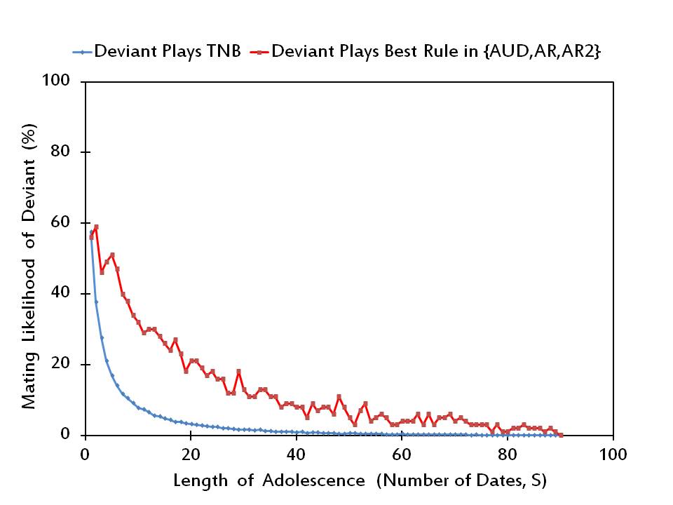
Figure 3. The mating likelihood of a potential deviant when he/she plays TNB versus the best alternative rule, while the rest of the society plays TNB. - 3.6
- It is apparent in Figure 3 that rTNB is not a Nash equilibrium profile for any value of S = 2, 3, …, 89. This result is not surprising since unlike the other rules TNB makes adjustments always in the upward direction and it does not depend on whether the potential deviant is found desirable by his/her date. Therefore, the aspiration level of a potential deviant in the mating phase is higher under TNB than under the alternative adjustment rules. Since the lower the aspiration level of an individual, the more likely he/she will accept a proposal in the mating period, an individual can increase his/her likelihood of mating by switching from TNB to the best alternative strategy in ℜ.
- 3.7
- In Figure 4 we show that rAUD is not a Nash equilibrium profile for short lengths of adolescence (S ≤ 32). For higher lengths of adolescence, rAUD may turn out to be a Nash equilibrium profile. Yet, this is only true for 28 out of all values of S between 33 and 90.
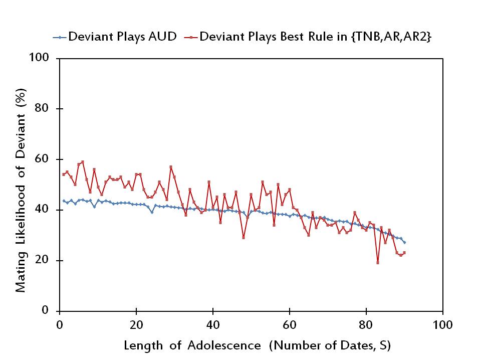
Figure 4. The mating likelihood of a potential deviant when he/she plays AUD versus the best alternative rule, when the rest of the society plays AUD. - 3.8
- A closer inspection of the simulation data generating Figure 4 also reveals that a randomly selected individual prefers to play Adjust Relative at 50 values and Adjust Relative/2 at only 12 values out of a total of 62 distinct values of S at which he/she finds it optimal to deviate from the Adjust Up/Down Rule.
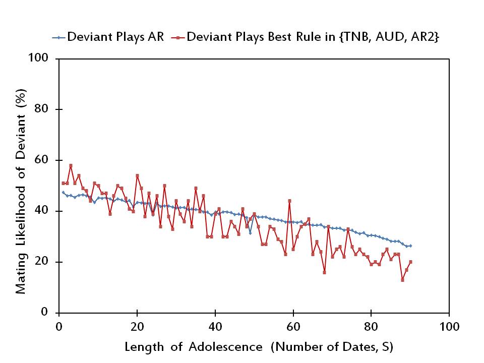
Figure 5. The mating likelihood of a potential deviant when he/she plays AR versus the best alternative rule, when the rest of the society plays AR. - 3.9
- In Figure 5, we illustrate that rAR is a Nash equilibrium profile for most of the medium to high lengths of adolescence (i.e., for 48 values of S exceeding 30). For most of the short lengths of adolescence (i.e., for 22 out of the lowest 30 values of S) an arbitrary individual has an incentive to unilaterally deviate from playing Adjust Relative. Only at 6 out of 34 values of S where rAR is not a Nash equilibrium, the deviating individual prefers to play Adjust Up/Down, while he/she plays Adjust Relative/2 in the remaining 28 instances.
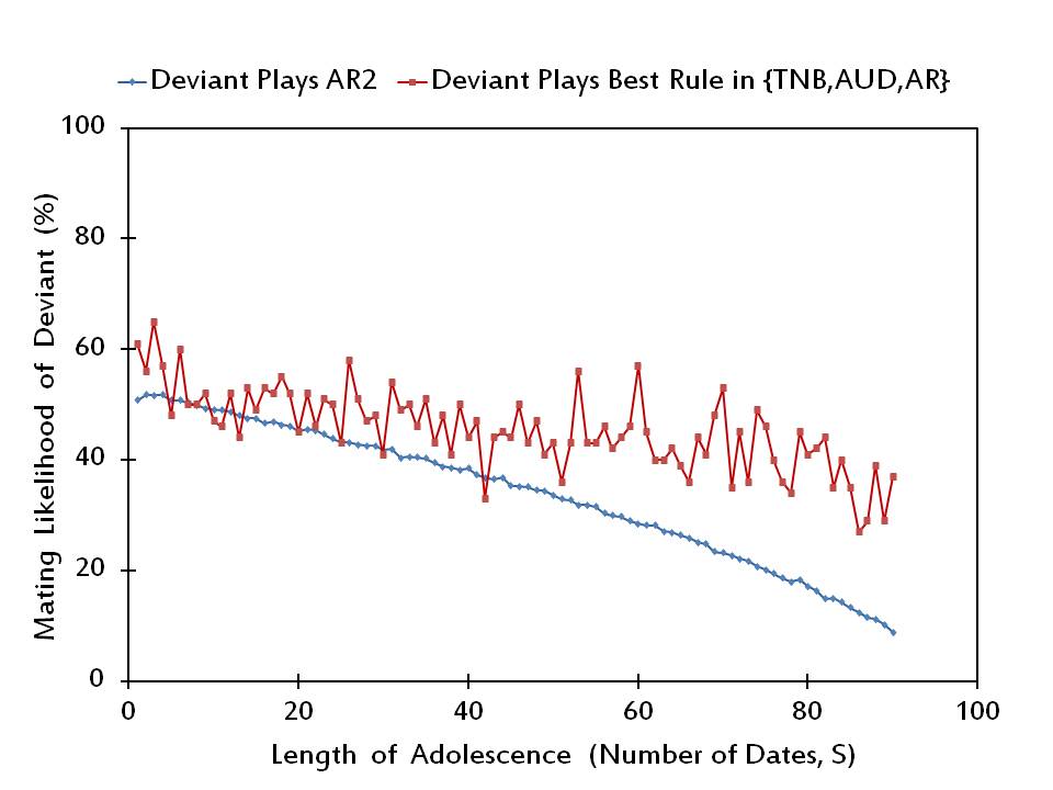
Figure 6. The mating likelihood of a potential deviant when he/she plays AR2 versus the best alternative rule, when the rest of the society plays AR2. - 3.10
- Finally, in Figure 6 we plot the equilibrium results for Adjust Relative/2. Here, we find that rAR2 is not a Nash equilibrium for 81 out of 90 values of S, while most of the remaining 9 values supporting an equilibrium are small. Moreover, the deviating individual prefers to play Adjust Relative in 63 out of 81 values of S at which rAR2 is not a Nash equilibrium, whereas he/she plays Adjust Up/Down in the remaining 18 cases.
- 3.11
- It is natural to ask here why the strategy profile rAR2 turns out to be the most successful profile in terms of the Nash stability. One possible explanation may be related to the variance of aspirations generated by alternative strategy profiles. We observe that although the profiles rAUD, rAR, and rAR2 yield almost the same mean aspiration level, close to the mean mate value of 50, for almost all adolescence lengths, the standard deviation of aspiration around the mean value is significantly different for these profiles, as reported below for a sample of values of S.
Table 2: The mean value of the standard deviation of aspiration levels under the profiles rAUD, rAR, and rAR2 S rAUD rAR rAR2 10 34.61 16.55 24.73 30 34.84 16.73 27.92 50 34.67 16.98 28.48 70 34.56 16.81 28.64 90 34.70 16.76 28.63 - 3.12
- In the above table, the standard deviation of aspirations is lower under the profiles rAR (around 16) and rAR2 (between 24-29) than under rAUD (around 34) since not only that the former rules allow the possibility of nonadjusting the aspiration after a date, but also the conditions for adjusting it are stronger (as the mutual desirability of the dating partners is required). On the other hand, the reason why rAR and rAR2 themselves yield significantly different standard deviations of aspirations should be the difference of the size of adjustments in the definition of these two profiles. Considering our findings, it seems that the smaller the variance of aspirations generated by a particular strategy profile, the more likely its survival against the alternative strategies of potential deviants.
- 3.13
- From our simulation results, we also see that for a majority of adolescence lengths, the Adjust Relative Rule is the best strategy of a deviant at both of the profiles rAUD and rAR2. This is so, despite the observation in Figure 1 that Adjust Up/Down dominates the Adjust Relative and Adjust Relative/2 Rules in terms of the induced likelihood of mating, for more than half of the considered values of S (i.e., for 54 values between S = 36 and S = 90). Interestingly, these two rules that are inferior to Adjust Up/Down for a majority of adolescence lengths when they are played by the whole population can become superior to it for some adolescence lengths when they are played singly by any individual.
- 3.14
- We should immediately note the tension between the results in this section examining the behavioral stability (à la Nash equilibrium) of the four adjustment rules and the findings in Figure 2 that give insights about the expected stability of the mating outcomes generated by the same rules. While the adjustment rule that is most favored by behavioral selection seems to be Adjust Relative, the stability of the mating as measured by the average assortativeness points to Adjust Relative/2 as the most successful rule among the three rules that all dominate the TNB rule in terms of likelihood of mating. The inconclusive rivalry between the Adjust Relative and Adjust Relative/2 Rules along with the observation in Figure 1 that no rule among Adjust Up/Down, Adjust Relative and Adjust Relative/2 dominates the rest with respect to the likelihood of mating indicates the need for assessing the adjustment rules using an integrative metric. Thus, we combine three distinct measures to get an aggregate measure πi, formally a function from the strategy profiles in R 2n to the reals, as follows:
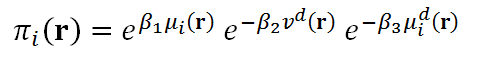
where β1, β2, β3 ∈ [0,1] are the weight parameters satisfying β1 + β2 + β3 = 1, πi( ℜ) denotes the mating likelihood of individual i at the profile r, vd(r) denotes the mean within-pair difference in mate value (normalized by the maximal mate value of 100) under the profile r, and μdi(r) denotes the marginal effect (on his/her mating likelihood) of his/her deviating from the strategy ri at the profile r to the best deviating strategy ri*( r-i); i.e.
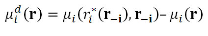
with r*i(r−i) = argmaxr'∈R\{ri} μi(r', r-i).
- 3.15
- The first exponential term above captures the positive relation between the payoff of an individual and his/her likelihood of mating. The second exponential term stands for the payoff from the expected stability of the mating outcome measured by the assortativeness of the mating. The higher the similarity of pairs (i.e., the smaller the mean within-pair difference in mate value), the higher this exponential term and consequently the higher the aggregate payoff. Finally, the third term represents the marginal payoff an individual can secure by not deviating from the heuristic followed by the whole population. Note that the smaller is the value of μdi(r), the higher is the likelihood that the profile r will survive as a Nash equilibrium in strategic plays, hence the higher will be the aggregate payoff πi(r).
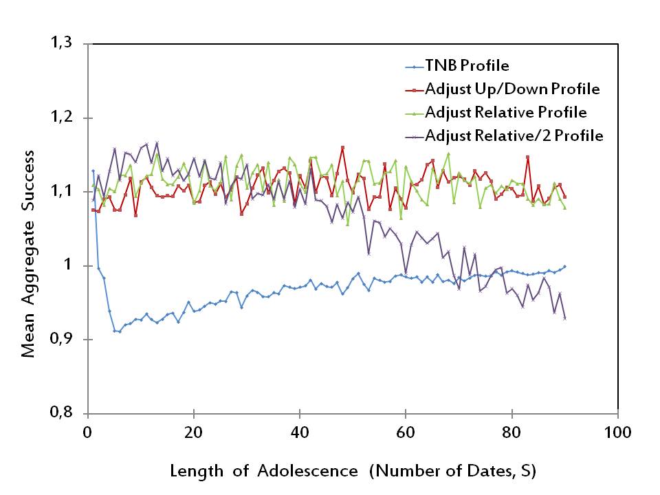
Figure 7. Mean Aggregate Success of Alternative Strategy Profiles (β1 = β2 = β3 = 1/3) - 3.16
- In Figure 7, we plot the performances of the four strategy profiles rTNB, rAUD, rAR, and rAR2 with respect to the aggregate success measure πi for the special case in which the three distinct measures in πi have equal weights, i.e., β1 = β2 = β3 = 1/3. We observe that rAR2 yields the highest aggregate success for most of the short lengths of adolescence (exactly, for 23 out of the first 30 values of S). On the other hand, for higher lengths of adolescence, the most successful profile is either rAUD or rAR (each being superior for exactly half of the values of S between 31 and 90).
- 3.17
- Below, we will explore whether the particular result in Figure 7 is robust to the changes in the weight parameters β1, β2, and β3. To this end, we will estimate the performances of the four strategy profiles over a fine grid of the parameter space. Formally, for each β1 in the set {0, 0.1, 0.2, … , 1.0}$ we will change β2 in the set {0, 0.1, 0.2, … , 1- β1}. For each pair of (β1, β2) constructed in this way, the value of β3 will be determined as 1- β1- β2 , by assumption. Thus, we will have 66 distinct combinations of (β1, β2, β3). For each of these combinations, we report in Table 3 the count of adolescence lengths (in short, the success count) in {1, 2, … , 90} at which the profile r ∈ {rTNB, rAUD, rAR, rAR2} yields the highest mean aggregate success. We can immediately check that the result of equal weights in Figure 7, which primarily points to the profiles rAR and rAUD, extends to a wide part of the simulation range. Indeed, we find that the profile rAR yields the highest success in almost half of the parameter space for 32 out of 66 parameter points whereas the profile rAUD performs as the second-best profile, producing the highest success at 27 parameter points. On the other hand, one can predict using Figures 1 and 2 (or the original findings of Todd and Miller 1999) that the profile rAR2 may outweigh the profiles rAUD and rAR, if one puts an extremely high weight on the mean within-pair-difference in mate value. Evidently, we can confirm this fact in Table 3, checking the rows with (β1, β2)= (0.1,0.8), (0.1,0.9), or (0.2,0.8).
- 3.18
- A closer examination of Table 3 will allow us to derive the effects of independent weight parameters β1 and β2 on the success count of the two competing profiles rAR and rAUD. One can check that for all β1, the success count of the profile rAR is nonincreasing in β2. However, the success count of the profile rAUD is not monotonically changing with β2; it is nondecreasing in β2 if β1 ≥ 0.6 and nondecreasing in β2 only at small values of β2 (i.e., β2 ≤ 0.4) if β1 ≤ 0.5. To find the effects of β1 on the success counts of rAUD and rAR, one can sort the rows in Table 3 first with respect to β2 and then with respect to β1 (as in Table 4) to obtain that the profile rAR is nonincreasing in β1 for all β2 ≥ 0.1 whereas the profile rAUD is nondecreasing in β1 if β2 ≤ 0.3 and almost everywhere nondecreasing in β1 if β2 ≥ 0.4. Overall, our findings reveal that rAR performs as the best profile when both of the two measures, the mating likelihood of individual i and the mean within-pair difference in mate value, have sufficiently low weights in the mean aggregate success measure πi. Oppositely, when both of these two measures have high weights, rAUD becomes the most successful profile.
Table 3: The count of adolescence lengths in {1, 2, … , 90} at which the profile in {rTNB, rAUD, rAR, rAR2} yields the highest mean aggregate success (Data is sorted first with respect to β1 and then with respect to β2.) β1 β2 β3 rTNB rAUD rAR rAR2 β1 β2 β3 rTNB rAUD rAR rAR2 0 0 1 2 14 63 11 0.3 0.3 0.4 1 26 42 21 0 0.1 0.9 2 14 63 11 0.3 0.4 0.3 1 38 28 23 0 0.2 0.8 2 15 61 12 0.3 0.5 0.2 0 49 14 27 0 0.3 0.7 2 17 59 12 0.3 0.6 0.1 0 56 1 33 0 0.4 0.6 2 20 55 13 0.3 0.7 0 0 45 1 44 0 0.5 0.5 10 20 46 14 0.4 0 0.6 1 14 59 16 0 0.6 0.4 19 24 29 18 0.4 0.1 0.5 1 17 55 17 0 0.7 0.3 37 18 14 21 0.4 0.2 0.4 1 23 44 22 0 0.8 0.2 58 6 2 24 0.4 0.3 0.3 1 32 33 24 0 0.9 0.1 66 6 0 18 0.4 0.4 0.2 1 47 16 22 0 1 0 81 9 0 0 0.4 0.5 0.1 0 58 1 31 0.1 0 0.9 2 14 63 11 0.4 0.6 0 0 50 0 40 0.1 0.1 0.8 2 14 63 11 0.5 0 0.5 1 15 57 17 0.1 0.2 0.7 2 15 61 12 0.5 0.1 0.4 1 20 47 22 0.1 0.3 0.6 2 19 55 14 0.5 0.2 0.3 1 30 34 25 0.1 0.4 0.5 1 22 51 16 0.5 0.3 0.2 1 46 18 25 0.1 0.5 0.4 0 30 40 20 0.5 0.4 0.1 1 56 2 31 0.1 0.6 0.3 0 42 25 23 0.5 0.5 0 0 55 0 35 0.1 0.7 0.2 0 50 12 28 0.6 0 0.4 1 16 52 21 0.1 0.8 0.1 1 43 0 46 0.6 0.1 0.3 1 29 36 24 0.1 0.9 0 7 13 0 70 0.6 0.2 0.2 1 43 21 25 0.2 0 0.8 1 14 64 11 0.6 0.3 0.1 1 54 6 29 0.2 0.1 0.7 1 15 62 12 0.6 0.4 0 1 55 0 34 0.2 0.2 0.6 1 18 56 15 0.7 0 0.3 1 23 42 24 0.2 0.3 0.5 1 22 51 16 0.7 0.1 0.2 1 41 23 25 0.2 0.4 0.4 1 29 40 20 0.7 0.2 0.1 1 52 9 28 0.2 0.5 0.3 0 42 25 23 0.7 0.3 0 1 55 0 34 0.2 0.6 0.2 0 52 11 27 0.8 0 0.2 1 36 28 25 0.2 0.7 0.1 0 50 1 39 0.8 0.1 0.1 1 50 13 26 0.2 0.8 0 0 41 0 49 0.8 0.2 0 1 56 0 33 0.3 0 0.7 1 14 63 12 0.9 0 0.1 1 48 15 26 0.3 0.1 0.6 1 15 59 15 0.9 0.1 0 1 56 1 32 0.3 0.2 0.5 1 21 52 16 1 0 0 1 54 6 29 Table 4: The count of adolescence lengths in {1, 2, … , 90} at which the profile in {rTNB, rAUD, rAR, rAR2} yields the highest mean aggregate success (Data is sorted first with respect to β2 and then with respect to β1.) β2 β1 β3 rTNB rAUD rAR rAR2 β2 β1 β3 rTNB rAUD rAR rAR2 0 0 1 2 14 63 11 0.3 0.3 0.4 1 26 42 21 0 0.1 0.9 2 14 63 11 0.3 0.4 0.3 1 32 33 24 0 0.2 0.8 1 14 64 11 0.3 0.5 0.2 1 46 18 25 0 0.3 0.7 1 14 63 12 0.3 0.6 0.1 1 54 6 29 0 0.4 0.6 1 14 59 16 0.3 0.7 0 1 55 0 34 0 0.5 0.5 1 15 57 17 0.4 0 0.6 2 20 55 13 0 0.6 0.4 1 16 52 21 0.4 0.1 0.5 1 22 51 16 0 0.7 0.3 1 23 42 24 0.4 0.2 0.4 1 29 40 20 0 0.8 0.2 1 36 28 25 0.4 0.3 0.3 1 38 28 23 0 0.9 0.1 1 48 15 26 0.4 0.4 0.2 1 47 16 26 0 1 0 1 54 6 29 0.4 0.5 0.1 1 56 2 31 0.1 0 0.9 2 14 63 11 0.4 0.6 0 1 55 0 34 0.1 0.1 0.8 2 14 63 11 0.5 0 0.5 10 20 46 14 0.1 0.2 0.7 1 15 62 12 0.5 0.1 0.4 0 30 40 20 0.1 0.3 0.6 1 15 59 15 0.5 0.2 0.3 0 42 25 23 0.1 0.4 0.5 1 17 55 17 0.5 0.3 0.2 0 49 14 27 0.1 0.5 0.4 1 20 47 22 0.5 0.4 0.1 0 58 1 31 0.1 0.6 0.3 1 29 36 24 0.5 0.5 0 0 55 0 35 0.1 0.7 0.2 1 41 23 25 0.6 0 0.4 19 24 29 18 0.1 0.8 0.1 1 50 13 26 0.6 0.1 0.3 0 42 25 23 0.1 0.9 0 1 56 1 32 0.6 0.2 0.2 0 52 11 27 0.2 0 0.8 2 15 61 12 0.6 0.3 0.1 0 56 1 33 0.2 0.1 0.7 2 15 61 12 0.6 0.4 0 0 50 0 40 0.2 0.2 0.6 1 18 56 15 0.7 0 0.3 37 18 14 21 0.2 0.3 0.5 1 21 52 16 0.7 0.1 0.2 0 50 12 28 0.2 0.4 0.4 1 23 44 22 0.7 0.2 0.1 0 50 1 39 0.2 0.5 0.3 1 30 34 25 0.7 0.3 0 0 45 1 44 0.2 0.6 0.2 1 43 21 25 0.8 0 0.2 58 6 2 24 0.2 0.7 0.1 1 52 9 28 0.8 0.1 0.1 1 43 0 46 0.2 0.8 0 1 56 0 33 0.8 0.2 0 0 41 0 49 0.3 0 0.7 2 17 59 12 0.9 0 0.1 66 6 0 18 0.3 0.1 0.6 2 19 55 14 0.9 0.1 0 7 13 0 70 0.3 0.2 0.5 1 22 51 16 1 0 0 81 9 0 0
Conclusions
- 4.1
- In this paper, we have studied whether some simple decision heuristics in the two-sided human mate search are behaviorally stable with respect to the Nash equilibrium concept. We have restricted our focus to four heuristics (aspiration adjustment rules), namely the TNB, Adjust Up/Down, Adjust Relative, and Adjust Relative/2 Rules, which were initially considered by Todd and Miller (1999). Using a two-phase search model of theirs, which involves an adolescence phase and a mating phase, we have showed that in the whole simulation range of adolescence lengths, the unanimous use of the TNB Rule by the whole population never arises as an equilibrium of a strategic game played right before the adolescence phase. Of the other three rules that all dominate TNB but no other rule in terms of likelihood of mating, Adjust Up/Down and Adjust Relative/2 have been observed as an equilibrium play, though only for a small part of the simulation range; the former arising when the adolescence is long and the latter arising when the adolescence is short. On the other side, the Adjust Relative Rule has been found to be behaviorally stable for a great part of the simulation range, especially for medium to high adolescence lengths.
- 4.2
- Taking stock of our results, the stability of heuristics as a new measure of mating success points to that among the mate search rules we have considered, the Adjust Relative Rule appears to be the one which is most likely to be favored by strategic selection. On the other hand, the stability of the mating outcome, as measured by the assortativenes of the mating, indicates the superiority of the Adjust Relative/2 Rule (Todd and Miller 1999, and Figure 2). Apparently, the lists of rankings of the four adjustment rules are not identical with respect to the three metrics, involving the likelihood of mating, the behavioral (strategic) stability of the adjustment rule and the stability of the mating outcome measured by the assortativeness of the mating. To balance the outcomes of these three metrics, we have combined them to obtain an aggregate payoff function. By changing the weights of the three metrics in this aggregate payoff function, we have tested the performances of the four strategy profiles. Our findings show that for almost half of the possible representations of our aggregate measure, the highest success is attained by the Adjust Relative Rule, closely followed by the Adjust Up/Down Rule.
- 4.3
- We believe that the contribution of this study to the previous literature on mate search is at least twofold. First, we add some new results to a very thin literature dealing with the stability issues in agent-based search models. Thereby, we hope to narrow down the existing gap between the priorities of stable matching theory and agent-based mate search. However, unlike the previous works (Eriksson and Hägsström 2008; Eriksson and Strimling 2009), our main focus is on the stability of mate search heuristics, using the Nash equilibrium concept, instead of the stability of the mating outcome in the usual definitions of blocking individuals or pairs. Second, since a particular search heuristic can be behaviorally stable only if no individual in the population has an incentive to unilaterally switch to an alternative heuristic, our results shows the robustness of search heuristics considered by Todd and Miller (1997, 1999) with respect to the assumption that the whole population uses the same particular heuristic during the mate search.
- 4.4
- One potential criticism to our study, which deals with the stability of simple heuristics in a model with assumedly nonoptimizing individuals, could be that we restrict our stability notion to an `intelligent' concept such as Nash equilibrium. This concept requires that the beliefs of each individual about what strategies are likely to be played by other individuals are common knowledge and also that each individual is endowed with the skill of performing optimization over the outcomes of alternative strategies. However, our appeal to the Nash equilibrium concept is not wholly illegitimate. An observation that the play of a particular heuristic by the whole population is not a Nash equilibrium would directly point to the existence of a better heuristic from the viewpoint of a unilaterally deviating individual. Clearly, such an individual could find the merit of playing this alternative heuristic also under the notion of evolutionary stable strategies introduced by Maynard Smith and Price (1973) and Maynard Smith (1974). In their evolutionary model, nonoptimizing individuals (players) may deviate from a particular common (incumbent) rule only because they are programmed to do so or alternatively by `simple' or `unsophisticated' reasons, involving mistakes, ignorance, etc, simply called `mutations'.[8]
- 4.5
- We should finally note that the future research may profitably study a broader model where each individual in the mating population is set free to use any available search rule during the mate search, independent from the set of rules used by other individuals. Constructing such a heterogenous model of mate search, one may find the efficient distributions of search rules over a given mating population that will optimize a particular measure of mating success. Using the approach in this paper, one could also search for strategically stable distributions of search rules, and in particular the strategically stable distributions among the efficient ones.
Acknowledgements
-
The author thanks two anonymous reviewers for very helpful remarks and suggestions that have greatly changed the paper, and thanks Dr. Mehmet Yigit Gurdal for fruitful discussions as well as for his kind help in the computer simulations. The author also acknowledges the financial research support of the Turkish Academy of Sciences. The usual disclaimer applies.
Notes
-
1 See Abdulkadiroğlu and Sönmez (Abdulkadiroğlu 2003) for a pioneering work, and Abdulkadiroğlu (2013) and Pathak (2011) for surveys, on school choice, and Roth and Sotomayor (1990) for a wide range of earlier results in stable matching theory.
2 Stable matching theory was applied to study the formation/dissolution of marriages only very recently by Mumcu and Saglam (2008) for the case of transferable utilities and by Saglam (2013) for the case of nontransferable utilities.
3 See Kalick and Hamilton (1986) for an early example of computer-based, decentralized and sequential models of mate search.
4 An important feature of that model is that individuals have common preferences for the opposite sex, i.e., they hold a universal notion of attractiveness. Therefore, mate value of each individual is the same in the eyes of all other individuals. More recent agent-based models of French and Kus (2008) and Hills and Todd (2008) allow for heterogenous preferences.
5 The adjustment rules considered by Todd and Miller (1999) also involve the Mate Value-α Rule, according to which the aspiration level of each individual is constant over the adolescence period and formed by subtracting a prescribed constant α (picked as 5 in their simulations) from one's self mate value. We exclude this rule from the scope of our paper since it requires, as already noted by Todd and Miller (1999), that each individual knows his/her self mate value, a highly unrealistic assumption.
6 Both sociology and psychology involve studies accepting the view that humans are inclined to mate with others similar to themselves in physical and personality attributes, nationality, religion, geography, age, educational, occupational and social status (Alvarez and Jaffe 2004; McPherson et al. 2001; Miller and Todd 1998). Clearly, under this view, the rate of divorce for the purpose of remarriage is lower in populations with a high percentage of assortatively mated pairs. Recently, an agent-based marriage and divorce model of Hills and Todd (2008), called MADAM, explored the empirical validity of (homophilic) assortativeness in human mate search. This model, involving individuals with multiple traits and time-relaxing expectations, shows that the increase in the population heterogeneity when individuals mate assortatively can explain the dynamic patterns of the marriage and divorce hazard rates for New Zealand, Iceland, and England observed in the past.
7 In the secretary problem, an employer must hire the best applicant for a secretarial job, interviewing each applicant one at a time without being able to make a job offer to an already interviewed applicant. The employer knows the number of applicants but does not know the distribution of the applicants. In this setup, the optimal strategy of the employer turns out to be first interviewing (approximately) 37% of the available applicants and choosing in the following hiring period the next better applicant whose quality is above the quality of the best applicant interviewed. The TNB Rule considered by Todd (1997) and Todd and Miller (1999) is similar to the search rule in the secretary problem except for that (i) the number of potential mates does not need to be known by any individual searching for a mate and (ii) individuals do not optimize but use heuristics they find to be satisficing.
8 In the evolutionary model of Maynard Smith and Price (1973) and Maynard Smith (1974), an incumbent strategy is called evolutionary stable if for each mutant strategy there exists a threshold such that the incumbent strategy yields a higher fitness (payoff) than the mutant strategy when the share of individuals playing the mutant strategy is below this threshold. Since each evolutionary stable strategy must be trivially optimal against itself, the set of evolutionary stable strategies are always contained by the set of Nash equilibria.
References
-
ABDULKADIROĞLU, A. (2013) School choice. In Z. Neeman, M. Niederle & N. Vulkan (Eds.), Oxford Handbook of Market Design, forthcoming. [doi:10.1093/acprof:oso/9780199570515.003.0006]
ABDULKADIROĞLU, A. & Sönmez, T. (2003) School choice: A mechanism design approach. American Economic Review, 93, 729–747. [doi:10.1257/000282803322157061]
ALVAREZ, L. & Jaffe, K. (2004) Narcissism guides mate selection: Humans mate assortatively, as revealed by facial resemblance, following an algorithm of ``self seeking like". Evolutionary Psychology, 2, 177–194. [doi:10.1177/147470490400200123]
APTECH SYSTEMS. (1998) GAUSS version 3.2.34. Maple Valley, WA: Aptech Systems, Inc.
BECKAGE, N., Todd, P., Penke, L. & Asendorpf, J. (2009) Testing sequential patterns in human mate choice using speed-dating. In N. Taatgen & H. van Rijn (Eds.), CogSci 2009 Proceedings (pp. 2365–2370).
COLLINS, E. J., McNamara, J. M. & Ramsey, D. M. (2006) Learning rules for optimal selection in a varying environment: Mate choice revisited. Behavioral Ecology, 17, 799–809. [doi:10.1093/beheco/arl008]
DAWKINS, R. (1976) The Selfish Gene. Oxford: Oxford University Press.
DOMBROVSKY, Y. & Perrin, N. (1994) On adaptive search and optimal stopping in sequential mate choice. American Naturalist, 144, 355–361. [doi:10.1086/285680]
ERIKSSON, K. & Häggström, O. (2008) Instability of matchings in decentralized markets with various preference structures. International Journal of Game Theory, 36, 409–420. [doi:10.1007/s00182-007-0081-6]
ERIKSSON, K. & Strimling, P. (2009) Partner search heuristics in the lab: Stability of matchings under various preference structures. Adaptive Behavior, 17, 524–536. [doi:10.1177/1059712309341220]
FAWCETT, T. W., Hamblin, S. & Giraldeaub, L.-A. (2012) Exposing the behavioral gambit: The evolution of learning and decision rules, Behavioral Ecology, 24(1), 2–11. [doi:10.1093/beheco/ars085]
FERGUSON, T. S. (1989) Who solved the secretary problem? Statistical Science, 4, 282–296. [doi:10.1214/ss/1177012493]
FRENCH, R. M. & Kus, E. T. (2008) KAMA: A temperature-driven model of mate choice using dynamic partner preferences. Adaptive Behavior, 16, 71–95. [doi:10.1177/1059712307087598]
GALE, D. & Shapley, L. S. (1962) College admissions and the stability of marriage. American Mathematical Monthly, 69, 9–15. [doi:10.2307/2312726]
GIGERENZER, G., Todd, P. M., & the ABC Research Group (1999) Simple Heuristics That Make Us Smart. New York: Oxford University Press.
GIRALDEAU, L-A, Dubois, F. (2008) Social foraging and the study of exploitative behavior. Advances in the Study of Behavior, 38, 59–104. [doi:10.1016/S0065-3454(08)00002-8]
HILLS, T. & Todd, T. (2008) Population heterogeneity and individual differences in an assortative agent-based marriage and divorce model (MADAM) using search with relaxing expectations. Journal of Artificial Societies and Social Simulation, 11(4), 5. https://www.jasss.org/11/4/5.html.
KALICK, S. M., & Hamilton, T. E. (1986) The matching hypothesis reexamined. Journal of Personality and Social Psychology, 51, 673–682. [doi:10.1037/0022-3514.51.4.673]
MAYNARD SMITH, J. (1974) The theory of games and the evolution of animal conflicts. Journal of Theoretical Biology, 47, 209–221. [doi:10.1016/0022-5193(74)90110-6]
MAYNARD SMITH, J. (1982) Evolution and the Theory of Games. Cambridge, UK: Cambridge University Press. [doi:10.1017/CBO9780511806292]
MAYNARD SMITH, J. & Price, G. R. (1973) The logic of animal conflict. Nature, 246, 15–18. [doi:10.1038/246015a0]
MAZALOV, V., Perrin, N. & Dombrovsky, Y. (1996) Adaptive search and information updating in sequential mate choice. American Naturalist, 148, 123–137. [doi:10.1086/285914]
MCPHERSON, M., Smith-Lovin, L., & Cook, J. M. (2001) Birds of a feather: Homophily in social networks. Annual Review of Sociology, 27, 415–444. [doi:10.1146/annurev.soc.27.1.415]
MILLER, G. F. & Todd, P. M. (1998) Mate choice turns cognitive. Trends in Cognitive Sciences, 2, 190–198. [doi:10.1016/S1364-6613(98)01169-3]
MUMCU, A. & Saglam, I. (2008) Marriage formation/dissolution and marital distribution in a two-period economic model of matching with cooperative bargaining. Journal of Artificial Societies and Social Simulation, 11(4), 3. https://www.jasss.org/11/4/3.html.
NASH, J. (1950) Equilibrium points in n-person games. Proceedings of the National Academy of Sciences, 36, 48–49. [doi:10.1073/pnas.36.1.48]
PATHAK, P. A. (2011) The mechanism design approach to student assignment. Annual Reviews of Economics, 3, 513–536. [doi:10.1146/annurev-economics-061109-080213]
ROTH, A. E. (1984) The evolution of the labor market for medical interns and residents: A case study in game theory. Journal of Political Economy, 92, 991–1016. [doi:10.1086/261272]
ROTH, A. E. & Sotomayor, M. (1990) Two-Sided Matching: A Study in Game Theoretic Modeling and Analysis. Cambridge: Cambridge University Press. [doi:10.1017/CCOL052139015X]
SAGLAM, I. (2013) Divorce costs and marital dissolution in a one-to-one matching framework with nontransferable utilities. Games, 4, 106–124. [doi:10.3390/g4010106]
SEALE, D. A. & Rapoport, A. (1997) Sequential decision making with relative ranks: An experimental investigation of the "secretary problem". Organizational Behavior and Human Decision Processes, 69, 221–236. [doi:10.1006/obhd.1997.2683]
SIMÃO, J. & Todd, P. M. (2002) Modeling mate choice in monogamous mating systems with courtship. Adaptive Behavior, 10, 113–136. [doi:10.1177/1059712302010002003]
SIMÃO, J. & Todd, P. M. (2003) Emergent patterns of mate choice in human populations. Artificial Life, 9, 403–417. [doi:10.1162/106454603322694843]
SIMON, H. A. (1955). A behavioral model of rational choice. Quarterly Journal of Economics, 69, 99–118. [doi:10.2307/1884852]
TODD, P. M. (1997) Searching for the next best mate. In R. Conte, R. Hegselmann & P. Terna (Eds.), Simulating Social Phenomena (pp. 419–436). Berlin: Springer-Verlag. [doi:10.1007/978-3-662-03366-1_34]
TODD, P. M., Billari, F.C. & Simão, J. (2005) Aggregate age-at-marriage patterns from individual mate-search heuristics. Demography, 42, 559–574. [doi:10.1353/dem.2005.0027]
TODD, P. M. & Miller, G. F. (1999) From pride and prejudice to persuasion: Satisficing in mate search. In G. Gigerenzer, P. M. Todd & the ABC Research Group (Eds.), Simple Heuristics That Make Us Smart (pp. 287–308). New York: Oxford University Press.