
 Abstract
- We present a brief history of models of opinion dynamics in groups of agents, and summarise work from the creation of the Bounded Confidence model (Krause 2000; Hegselmann and Krause 2002) through to the more recent development of the Relative Agreement (RA) model (Deffuant et al. 2002; Deffuant 2006). In the RA model, randomly-selected pairs of agents interact, expressing their opinions and their confidence in those opinions; and each agent then updates their own opinion on the basis of the new information. The two seminal RA papers (Deffuant et al. 2002, Deffuant 2006), both published in JASSS, each present simulation results from the RA model that we have attempted to independently replicate. We have surveyed over 150 papers that cite Deffuant et al. 2002, yet have found no prior independent replications of the key empirical results for the RA model presented in the 2002 paper. We have each written a separate implementation of the RA model (one in Java, one in Python, both published in full as appendices to this paper) which we therefore believe to be the first independent replications of the RA model as published in the 2002 JASSS paper. We find that both our implementations of the RA model generate results that are in good agreement with each other, but both of which differ very significantly from those presented by Deffuant et al.. Our results are presented along with an analysis and discussion where we argue from first principles that our results are more plausible than those published in the 2002 JASSS paper. We close with discussion of the relevance of this model, along with future applicability.
- Keywords:
- Relative Agreement Model, Opinion Dynamics, Agent-Based Simulation
Opinion Dynamics and Consensus Formation
- 1.1
- From its initial coining, the term "opinion dynamics" has come to refer to a broad class of different models that can be applied to fields ranging from sociological phenomena to pure mathematics and the study of physics (Lorenz 2007). This paper however, will focus on models that are primarily linked to the study of the dynamics of political, religious and ideological extremist opinions and the circumstances under which those opinions can rise to dominance. More precisely, this paper will examine the development of various models in recent years aimed at helping to explain and understand the causes of extremist populaces, particularly in the last decade or two, that are linked with causing significant terrorist acts.
- 1.2
- Suppose a group of experts are tasked with reaching an agreement on a given subject. Initially, all the experts will possess an opinion of their own which may be quite similar to, vastly different from, or perhaps even identical to, some of their colleagues'. For simplicity, we assume that an individual's opinion can be represented as a real number marking a point on some bounded continuum. During the course of their meeting, the experts each present their opinion to the group in turn and at the end they modify their own opinion slightly, using a fixed weight, in light of the views of the others. If all opinions are deemed to be equal at the end of the meeting it can be said that a consensus has been reached, otherwise another meeting is required. Although it is intuitively expected that this highly stylised model will always reach a consensus (provided that a positive weight is used) as each expert iteratively modifies their own opinion toward that of their colleagues, it is worth noting that there is a strict proof of this convergence, given by de Groot (1974), because many subsequent models presented are based on this example.
- 1.3
- Although simple and highly stylised, the de Groot model has been examined in various papers (Chatterjee and Seneta 1977; Friedkin 1999) and has been the basis for many subsequent models when applied to various specific fields. Indeed, it is clear that this model has the potential to help develop tools to study causes and conditions for the existence of large extremist groups. The problem however, is that under the specifications of the de Groot model, a consensus is typically reached in the middle ground, that is to say, the consensus of the experts is merely an average of the initial opinions. Given the existence of real-world examples of countrywide populations or very large groups forming with extremist opinions, it is clear that although useful, the de Groot model does not yet succeed in explaining such occurrences. Clearly it could be argued that such occurrences are caused by forces outside of the scope of de Groot's model or indeed simply highlight the problems of applying idealised simulations directly to the real-world without giving consideration to the sometimes irrational behaviour of people. Conversely, there have also been several serious attempts at modification of de Groot's basic model to produce various realistic outcomes when provided with different initial parameters, some of which can produce results which, although potentially counter-intuitive, can be better applied to real-life scenarios.
Bounded Confidence Model
- 2.1
- Building on the de Groot model, Krause developed a variation in which the experts would only consider the opinions of others provided that they were not too dissimilar from their own (Krause 2000). This is the "Bounded Confidence" model, also known as the Hegselmann-Krause model. The reasoning behind this is quite simple: it adds the idea that an expert with a given opinion has a quantifiable conviction about that opinion. Without this addition, it is conceivable that in the de Groot model a group of experts could be assembled with initial opinions such that one expert with an initial opinion at one extreme could finish with a completely opposite opinion. (This would occur if a large group were assembled where all experts have an opinion at one extreme with the exception of one expert whose opinion is the complete opposite.) While this can and does occur in real life, the de Groot model implies that this would happen every time these circumstances transpired. With the new condition in the BC model, if an expert is sufficiently convinced of their own opinion, experts with vastly different opinions would simply be ignored. That is, if another expert's opinion does not fall within the bounds of the former's opinion confidence then it is disregarded. Under these conditions, it is clear that a consensus may not always be reached by the group of experts. In fact, Krause went further and allowed the agents varying levels of confidence in their own opinions—an individual weight on their own opinions. In Krause's model, some experts may be so confident in their own opinion that they will only consider opinions very close to their own while others will be open to considering more divergent opinions. Intuitively, this too is more analogous to reality. Not only does this add significant complexity to the model, with the additional parameter of each expert's individual weight on her own opinion, the model now includes significant heterogeneity (Krause 2000).
- 2.2
- For completeness, the formal specification of the Bounded Confidence (BC) model (as described by Hegselmann and Krause 2002), is summarised here. We suppose that the group we are studying is comprised of n experts. The meetings that take place are represented by discrete time periods t = {0, 1, 2, …}. As stated in the previous section, we assume that each expert i (where 1 ≤ i ≤ n) possesses an opinion at each time period that can be expressed as a real number given by xi (t). Therefore x(t)represents a vector of all opinions held by all experts at time t. We can then define the opinion progression as:
xi (t+1) = a i1x1 (t) + a i2x2 (t) + … + ainxn (t) (1) where aij is the weighting between agent i and j, with aij ≥ 0 and a i1+ a i2+ … + ain = 1 making the progression a weighted average. It is also required that aii > 0 for all i, j, so that each agent assigns some nonzero value to their own opinion (Lorenz 2005). Nevertheless, by allowing weights to be zero-valued, we are allowing experts to disregard the opinions of others should they differ too much; although with weights being adjusted at each time step it is possible that an expert will come to accept another's opinion at a later time. The bounded nature of agents' confidence in this model is simply this: if an agent i is very confident in its own opinion, that is reflected in narrow bounds of tolerance on the difference in that agent's opinion and the opinion of another agent, for the other agent to influence the opinion of agent i; with less confidence, the bounds widen.
- 2.3
- When first presented in Krause (2000), few conclusions were drawn about the BC model, although Hegselmann and Krause (2002) gave a more thorough analysis with results from empirical explorations of the model via computer simulations. Although initially randomly spread, each simulation results in opinion clustering, where all agents split into initially a number of stable sub-groups with the same opinion in each sub-group. This is to be expected because if a group-wide consensus were found, even that would be considered as a single cluster. Unsurprisingly, it was also found that if the agents began with higher confidences (i.e. lower bounds on being influenced) the system would converge to a larger number of clusters. Clearly if the boundaries were set high enough, the simulation would act as the model described in the previous section. Once the asymmetry of agents having different levels of confidence in their own opinion was added, it was found that although similar results occur, it was possible for clusters to form nearer to extreme opinions. Generally, clusters would form around experts who started with initially high confidences (low bounds) and could therefore result in a single cluster reasonably near to an extreme end of the opinion scale. In a further experiment, simulations were performed to examine a reasonable assumption that experts with more extreme opinions would be more confident about those opinions (Hegselmann and Krause 2002). Depending on the parameters presented was typically found that two polarised clusters would form.
- 2.4
- With this success, it was clear that augmenting the agents with confidence in their own opinions was moving towards being better able to simulate extremist situations.
Relative Agreement Model
- 3.1
- After the BC model had been developed and while its properties were still being explored, another team of researchers led by Deffuant were developing what they named the Relative Agreement (RA) model, proposed as an extension to the BC model (Deffuant et al. 2002). There are two main differences between the BC and RA models. The first and arguably less significant different is how the agents interact. In the BC model all agents present their opinion in sequence which is followed by a group-wide evaluation of opinions, whereas in the RA model, pairs of agents are selected at random to interact. During an interaction, both agents present their opinion and then update their own opinion based on the opinion of the other. The second, more significant, change to the model is how each agent will update their opinion. In the BC model, an agent would only consider another agent's opinion provided that it fell within the bounds of its own opinion, as illustrated in Fig 1.
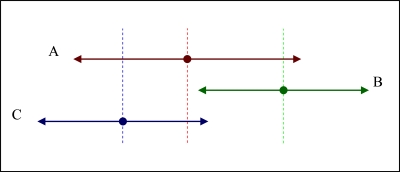
Figure 1. Agent interaction in the BC model: three agents ( A, B, and C) each have a particular opinion expressed as a point on a continuum—for clarity, the three agents are illustrated at different vertical heights, but conceptually all three lie on the same linear continuum. The "confidence zone" that each agent has in its own opinion, i.e. how susceptible each agent is to the influence of others, is represented by a bounded range to either side of its agent's opinion (illustrated as arrows to the left and right). For one agent X to influence the opinion of another agent Y, X's opinion point must be within the confidence bounds of Y. Thus, in this figure: B and C can both influence A; A can influence C but not B; B cannot influence C; and C cannot influence B. See text for further discussion. - 3.2
- We see in Figure 1 that Agent A has the lowest confidence in its opinion and therefore has the widest bounds. We can also see that Agent A will consider the opinion of both Agent B and Agent C at evaluation time, because both B and C's opinions lie within the opinion bounds of A. Clearly the opinion of agent B does not matter to agent C as B's opinions do not cross C's bounds. Note that while C will also consider the opinion of A, B will not as the opinion of A does not fall into the confidence zone of B. Now that we can know for any agent which opinions they will evaluate when generating their next opinion, we adjust them as before using a weighted sum. In the RA model, however, the weights are given by the size of the overlap between the two agents' boundaries as shown in Fig. 2 and are used to recalculate an agent's opinion and also its uncertainty (confidence) after the dual interaction.
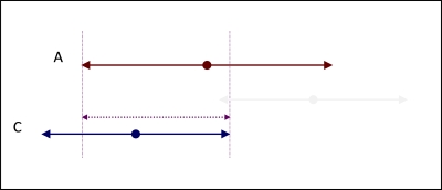
Figure 2. Agent interaction in the RA model. The degree of overlap between the confidence zones of the two agents is used to determine the weighting applied when updating opinions. - 3.3
- For completeness, a summary of the formal specification of the RA model is presented here, since this is the model that we examine in detail in the rest of this paper. We consider a group comprised of n agents. Each individual i possesses two variables; an opinion xi and an uncertainty ui, both of which are represented by a real numbers. The opinion of an individual is between 1.0 and -1.0 and its uncertainty is between 0.0 and 2.0. Randomly paired agent interactions are run until a stable population opinion state is reached. An agent interaction is calculated by first calculating the relative agreement between agents i and j by taking the overlap between the two agents' bounds hij, given by:
hij = min (xi + ui, xj + uj) -max(xi - ui, xj -uj) Followed by subtracting the size of the non-overlapping part given by:
2ui - hij So the total agreement between the two agents is given as:
hij - (2ui - hij) = 2(hij - ui) - 3.4
- Once that is calculated, the relative agreement is then given by:
2(hij - ui) / 2ui = (hij / ui) - 1 Then if hij > ui, then update of xj and uj is given by:
xj := xj + μ[(hij / ui) - 1](xi - xj) uj := uj + μ[(hij/ ui) - 1](ui - uj) where μ is a constant parameter that is responsible for controlling the speed of population convergence. When μ is low the population is less responsive to the opinions of others and when μ is high, a population will reach a convergence very quickly.
- 3.5
- The primary differences between the two models' specifications can be explained as a quest for increased realism. In a population, particularly a very large population, participants do not consider the opinion of every other member of that population. Therefore, the addition of the paired interactions makes good sense from a realism perspective although in practice it makes little difference to the outcome of the simulation. For this simulation to be run fairly, it must be running for a length of time such that the number of interactions that have taken place will allow stable clusters to form. The formation of stable clusters is caused by agents interacting with large numbers of other agents. In both models the agents will disregard opinions that are drastically different from their own and agree with opinions close to theirs, so over the course of an RA model simulation the interactions that take place will imitate the single group-wide interactions of the BC model. However, unlike the BC model, the asymmetries of influence dynamics in the RA model mean that it does not necessarily produce symmetric population-level results. The addition of the weights being linked to the proportion of agreement between the two agents makes complete sense: the nearer two agents are in agreement about their opinion and uncertainty, the more they should believe the other's opinion. The RA model's asymmetric influence rule, where agents that are more convinced of their own opinion are more persuasive to other agents (Deffuant 2006), also makes intuitive sense from a psychological perspective: uncertain people will probably not be as convincing as a person with a strong conviction.
Results of the RA Model
-
Comparison with the BC Model
- 4.1
- For their first set of simulations, Deffuant et al. tested how the model would perform under simple conditions. From there the model could be tested using more interesting values. The population was given random opinions between the range of 1.0 and -1.0 with identical uncertainties. The simulation was then repeated multiple times, exploring the effects of varying the uncertainty values. Deffuant et al. found that under these conditions the RA simulation performed in a manner that was very similar to the BC model. Typically the population converges to one or more stable clusters that are, on average, approximately the same size.
- 4.2
- Although not explicitly stated in any of literature on the RA model, it should also be noted that the population-wide opinion will always be close to 0. Indeed, over the course of one million simulation runs (performed to validate the results of the RA model under these parameters) the average population opinion was no further than ±0.1 from 0 on over 99.5% occasions and at no point did the average exceed ±0.2. Furthermore, over the course of the runs it became clear that the average would converge to 0. This is hardly surprising as the agents are initialised with random opinions distributed uniformly across the range. Therefore, we find that although stable clusters are forming, no actual population-wide shift occurs.
- 4.3
- Another observation that is worth noting from these experiments is that the number of clusters is linked to the initial uncertainty of the agents. Deffuant et al. stated the number of clusters found in the RA model would average around w/2u, where w is the width of the initial opinion distribution (between 1.0 and -1.0) and u is the initial uncertainty for the agents, which in this run was set to a constant. This is in contrast to the findings of the BC model where it was found that the number of clusters was better predicted as the integer floor of w/2u (Deffuant et al. 2000).
- 4.4
- The finding that the number of clusters is linked to the initial uncertainties is hardly surprising. Given that an agent will ignore an opinion outside the bounds of its confidence it feels quite reasonable that clusters would form with opinion distances approximately equal to twice the uncertainty. The reason for the doubling of the uncertainty is that the uncertainty value is applied both above and below the actual opinion of an agent. Therefore the range that an agent is willing to consider is 2u.
The RA model with Extremists
- 4.5
- Having demonstrated that the general results of the RA model were comparable to the BC model, Deffuant et al. (2002) added what they termed "extremist" agents to see if they could cause shifts in the opinions of entire population. An extremist agent was defined as an agent with an opinion above 0.8 or below -0.8 and a very low uncertainty. It follows that agents in possession of more extreme views are also more convinced of their opinion otherwise their views would be more moderate. This is a reasonable assumption that was also applied in subsequent work on the BC model (Hegselmann and Krause 2002). Conversely, a moderate agent is one whose opinion falls between 0.8 and -0.8 with a fixed, higher uncertainty who is therefore more willing to be persuaded by other agents.
- 4.6
- Deffuant argued that there were three possible outcomes from the simulation (Deffuant et al. 2002):
- The majority of the moderate agents converge towards the centre (central convergence);
- The body of moderate agents splits into two approximately equal sized groups one of which converges towards the positive and the other to the negative (bipolar convergence);
- The majority of the moderate agents converge towards a single extreme (single extreme convergence). In this case, it is not significant if the body converges to the positive or the negative as the dynamics behind these convergences are the same.
- 4.7
- As stated earlier, the details of the BC model published in Krause (2000) and Deffuant et al. (2002) showed that by modifying various input parameters it would be possible to increase the probability of central convergence and bipolar convergence, although single extreme convergence could not be simulated. Deffuant et al. aimed to discover how the RA model might allow for single extreme convergence. When the BC was modified in the manner presented by Hegselmann and Krause it became apparent that single extreme convergence did occur but only when the model's parameters were given very extreme values; and so the work of Deffuant et al. could also been seen as an attempt to produce single extreme convergence under more reasonable, more realistic, parameter-values.
Classifying Clustering
- 4.8
- Deffuant et al. defined the value y as a metric of the opinion clustering in a population of agents evolving over time according to the RA model. At the end of a simulation run, y is calculated by as
y = p'+2 + p'-2 where p'+ is the proportion of initially moderate agents that have finished with an opinion that is classified as extreme to the positive end of the scale and conversely p'- is given as the proportion of initially moderate agents that complete the simulation with an opinion classed as extreme-negative.
- 4.9
- For the characteristic classes of results of the simulation (i.e. central convergence, bipolar convergence and single extreme convergence) we find the y values as given by the following table.
Table 1: Convergence p'+ p'- y Central 0 0 0 Bipolar 0.5 0.5 0.5 Single Positive Extreme 1 0 1 Single Negative Extreme 0 1 1 - 4.10
- Deffuant et al. stated that this was an effective test to classify the results of a single run, but it should be noted that this is not always the case. For example, consider the case of a simulation run which results in a single extreme positive convergence, such that p'+ = 0.7 and p'- = 0. While intuitively we would be able to understand this to be a single convergence, in this case y = 0.49 thus classifying the run as a bipolar convergence. Clearly this is a very specific example, but it highlights that the problem with classifying the simulation run using only y, especially when considering that almost every simulation has some degree of variance through random fluctuations.
- 4.11
- One potential solution to this classification problem is to use the y value in addition to checking the final average group opinion. In our previous example, a genuine bipolar convergence would still have an average group opinion very close to 0, while we would expect that the single extreme convergence to have an average group opinion of close to 0.56 and no lower than 0.32. This however, is not a perfect solution since an extreme average group opinion for a bipolar convergence can reach as high as 0.55, although the likelihood of that occurring is very low. Therefore, using this extra value is only an extra assurance, not a guarantee. This improvement was later used by Deffuant (2006).
Convergence in the RA Model
- 4.12
- As would be expected, in simulations where extremist agents had little influence over the opinion of the other agents it was found that central convergence was a common occurrence; and in simulations where extremists held a large sway over the moderates, bipolar convergences and on occasion even single extreme convergences could occur. Parameters that control the degree of influence of extremist agents are: pe (the proportion of extremist agents); μ (the weight applied in addition to the relative agreement of another agent's opinion when an agent updates its own opinion); δ (the proportion of positive extremist agents compared with negative extremist agents); and ue and u (the uncertainties of extremist and moderate agents respectively). Many of the parameters were fixed for the majority of the initial simulations performed, typically: μ = 0.5, δ = 0, ue = 0.1 and N = 200.
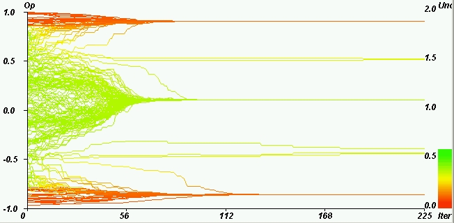
Figure 3. An example of central convergence with u = 0.4. Reproduced from Deffuant et al. (2002). The y-axis represents an agent's opinion while the colour represents the uncertainty of the agent (green is highly uncertain and red is confident). - 4.13
- In Fig 3 it can be seen that the majority of agents have converged toward the central opinion. This is the most common when initial uncertainties are low as the extremist agents are not as persuasive on the opinions of others. The reason behind this behavior is that when a moderate agent's uncertainty is initially that low, in order for there to be any agreement between an agent and a positive extremist agent, the agent must begin with an opinion of at least 0.4 (to reach the minimum positive extremist opinion of 0.8). In almost any case with u = 0.4, the average number of interactions for a moderate agent with other moderate agents will be higher than with extremists and there will be far more instances of agreement with other moderate agents than with extremists. Therefore the general result in these circumstances is that extremists are more or less ignored and the moderate agents converge toward the centre.
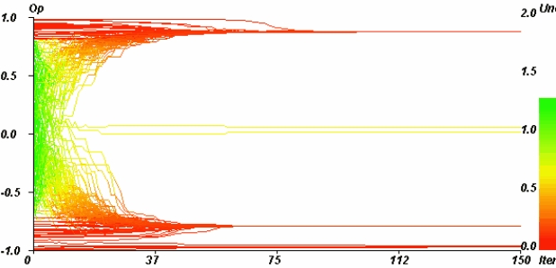
Figure 4. An example of bipolar convergence with u = 1.2. Reproduced from Deffuant et al. (2002) - 4.14
- When the uncertainty of the moderate agents is raised, we find that extreme agents are more persuasive to the moderate agents. This is because there is a far greater range of opinion that a typical agent is willing to consider. Under the parameter-values used for Fig. 4, an agent with an initial opinion of 0.0 would be willing to listen to the most extreme of both positive and negative extremist agents. As the extremist agents are generally more persuasive than moderate agents (due to their lower uncertainty) they then hold the most influence and this results in an approximately equal split of the population.
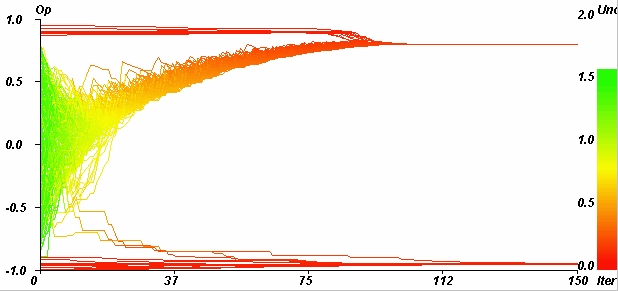
Figure 5. An example of single extreme convergence with u = 1.4. Reproduced from Deffuant et al. (2002). - 4.15
- Under very high uncertainties where virtually all of the moderate agents are willing to consider any extremist opinion, we see that an entire population can converge to a single extreme. That this result should have occurred at all was quite a surprise as it is rather counter intuitive and had not occurred in the work from which this model was based.
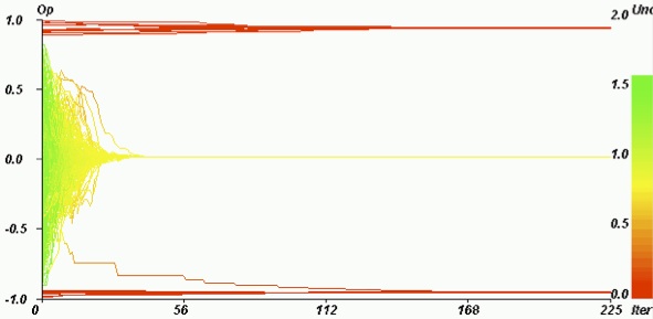
Figure 6. An example of central convergence occurring under parameters used in Fig 5. Reproduced from Deffuant et al. (2002). - 4.16
- When conditions are set to such extremes that they can produce outcomes as seen in Fig. 5 we also see that the other two types of convergence can occur. This variety of results demonstrates that these initial parameters make the "society" in the simulation interestingly unstable. To suggest that a society must be unstable in order for population-wide convergences to both or a single extreme is not particularly far-fetched. Indeed historically, countries that have experienced similar convergences have experienced sociological instability in some form. For instance, Germany in the 1930s converged to a single extreme after social unrest attributed to the signing of the Treaty of Versailles, the rise of the KPD (the German Communist Party), the Great Depression, etc. In the face of so much negativity the population faced high levels of uncertainty as to how the country could improve which led to the rise of an extremist power which affected the entire population. This could be seen as analogous to the uncertainty held by the agents in the model and the shows that the instability that arises in both can lead to extremist convergences.
- 4.17
- Following on from the success of finding clear, repeatable examples of single extreme convergence, Deffuant et al. set about testing all combinations of pe and u to see what typical y values were produced. For reasons that are not specified in their paper, the subsequent simulations also changed the value of μ to 0.2.
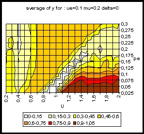
Figure 7. Average patterns of y with various u and pe. Reproduced from Deffuant et al. (2002). 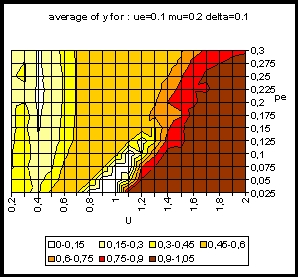
Figure 8. Average patterns of y with various u and pe with δ = 0.1. Reproduced from Deffuant et al. (2002). - 4.18
- A more complete interpretation of these results, comparing with those generated when trying to replicate them, can be found in the next section. At this stage, it suffices to say that the main finding of our re-implementation of this model was that, as δ increases, we find that in areas of instability the population becomes more likely to converge to the largest group of extremist agents. This is hardly surprising, as the larger that any one group becomes in comparison to the other, the more persuasive they become and the less persuasive the smaller one becomes.
Replication and Reproducibility
- 4.19
- In order to explore the work produced in Deffuant et al. (2002), we first set out to independently replicate he work presented in that paper. The first step was to ensure that our simulation demonstrated the three convergence types occurring in various areas of parameter-space. This proved itself to be a reasonably straightforward task: illustrative results from our simulation are presented in Figures 9, 10, and 11.
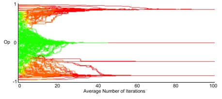
Figure 9. An example replication of results for central convergence. 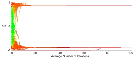
Figure 10. An example replication of results for bipolar convergence. 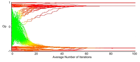
Figure 11. An example replication of results for the (uncommon) case of single extreme convergence. This graph highlights that, in our experience, the population converges to a single extreme only when the stochastic population dynamics favour one of the two extremes in early iterations. - 4.20
- Once our replication simulations had been developed to this point, one final test was needed to ensure their reliability: a comparison of typical values of y over the parameter space of pe and u as was illustrated in Deffuant et al.'s "heat-map" plots reproduced here in Figures 6 and 7 in the previous section. It was at this point that we found we could not replicate the results published by Deffuant et al. (2002). A comparison between our results and those of Deffuant et al. (2002) are illustrated in the heat-map plots of Figure 12.
- 4.21
- The original (u,pe) parameter-space heat-maps reproduced in Figures 6 and 7 show a very complex and apparently noisy pattern of average values of y. Furthermore, the original figures also show that the average value of y can reach values up to the maximum possible of 1; i.e. that all initially moderate agents finished converging to a single extreme. Given that the y value plotted in the heat-map is an average of fifty simulation runs, this suggests that over the course of the 50 simulation runs, every single run resulted in a single-extreme convergence. This seems to contradict Deffuant et al.'s earlier claims that single extreme convergence (SEC) can occur only under (u,pe) combinations that give initially uncertain populations, and that for SEC to be possible, the (u,pe) parameters should give sufficient instability that all three results (SEC, bipolar, and central convergence) have some likelihood of occurring. Thus it follows that although SEC can certainly occur in various areas of the parameter-space, the average y value could not be close to 1 because, if SEC can occur, then there should be some nonzero probability of bipolar and central convergences also occurring and hence the mean y value from a number of independent repetitions of the experiment should not reach 1, provided that sufficiently many samples have been taken to form a truly representative average.
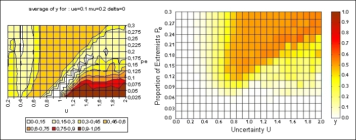
Figure 12. Conflicting (u,pe) "heat map" plots showing average values of y as u and pe are varied, using identical parameters for ue, µ and δ. The left-hand plot is copied from Deffuant et al. (2002); the right-hand plot is data from our simulation. The differences are significant, and are discussed further in the text. - 4.22
- In our replications of Deffuant et al.'s work using identical parameters, we see a much smoother gradation in the average value of y (i.e., the "heat"), with the average y-value peaking only at around 0.5. In the areas of (u,pe) parameter-space where mean y reaches 0.5, we found that instances of single extreme convergence also occurred. This is in agreement with our intuitive argument that in areas of parameter-space that allow single extreme convergence, the mean y-value would remain at a lower value due to the instability in the initial population leading not only to SEC but also to central and bipolar convergence. .
- 4.23
- One other very noticeable difference between the original results and those from our replications, apart from the maximum average y value being substantially different, is the extent of areas in the parameter-space at which high levels of instability occur. In the results presented by Deffuant et al. it is clear that instability occurs with higher initial general agent uncertainty. Our replications do agree with this, and intuitively also it is a relationship that seems to be borne out by historical evidence of sociological extremism too. Nevertheless, the difference between the original results and our replication in Deffuant et al.'s simulation the high y value occurs when pe is extremely low yet in our replications this only happens once pe is relatively high.
- 4.24
- Empirical evidence supporting either of these results would be hard to clarify. In many historical cases the pervading extremist minority has been very small in comparison to the population as a whole, and in these cases the reason the minority extremists have come to change the opinion of the population as a whole is because the members of the minority are in positions of power and influence. The RA model allows for agents that are more certain of their opinions to be more persuasive but it does not allow for agents (or groups of agents) to be more or less influential. This could possibly be rectified by allowing certain agents to have a higher bias in the random agent selection for the agent interaction, although a more comprehensive discussion of this refinement follows in the Further Work section, below. It could clearly be argued that the RA model emulates the effect of having higher influence by increasing pe, but the effect of increasing pe is simply that moderate agents are exposed to a greater number of extremist agents (although both positive and negative), which corresponds to a smaller number with a greater level of influence. On the basis of these observations, we believe that the results from our replication implementation of the RA model seem more natural, intuitive and justifiable than do those originally published by Deffuant et al.
- 4.25
- As a final demonstration of the problems present in Deffuant et al.'s published heat-maps, compared with the replication heat-maps presented in this paper, it is worth noting that there exists an area in Figure 12 that deserves detailed study. In the lower right hand segment of the figure (where all agents possess a moderate opinion and an uncertainty such that all other agents' opinions will be considered), the model is almost the same as the de Groot model save for the manner in which the agents interact, i.e. the model will perform identically to BC model without extremist agents. In the BC model without extremist agents, it was demonstrated that there was no single extreme convergence and indeed under these particular constraints a central consensus must always be reached. Indeed this has been proven mathematically and can be seen intuitively that if the only way for agents to update their opinion is toward each other then there is no way for a single agent, let alone the majority, to move outside the boundaries of the original maximal and minimal opinion values. Recall that when uncertainties are this high, every other agent's opinion will be agreed with (except in uninteresting cases of impractically low values μ) and so it becomes impossible for an agent to reject any opinion, thus hence agents are always moving towards a general consensus. In Figure 11 we see that Deffuant et al.'s claim that under these constraints the majority of agents will consistently converge to an initially non-existent extreme, something which is clearly not possible, while the results from our replication agree with the implications of de Groot's convergence proof and the findings of the BC model which state that a central convergence will be repeatedly reached.
- 4.26
- We believe that the reason for the differences present in our findings and those in Deffuant et al.'s work is most likely due to an accidental error on the part of Deffuant et al.. The two of us, the authors of this paper, have each run numerous simulations, from independent re-implementations (Meadows' written in Java, Cliff's in Python) of the formal model specification provided by Deffuant et al. that was summarised in Section 3. We used the same parameter-values as specified in Deffuant et al.'s paper and yet all our simulation-runs have resulted in results that show no significant differences between the Java and Python replications; while for both of us our results conflict with those presented by Deffuant et al. The source code for our Java and Python implementations is included in the Appendix, for completeness, and to encourage other authors to explore and replicate the results we present here.
Variations in number of agents
- 5.1
- Our next step was to test whether our heat-map results are sensitive to the number of agents n in the model system. The following graphs were generated using a series of tests running 50 i.i.d sample repetitions at each parameter setting testing n at 100 through to 1000, in increments of 50.
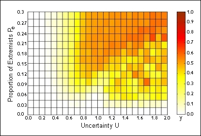
Figure 13. Heat-map showing mean value of y over (u,pe) parameter-space with n = 100. When pe is extremely low and uncertainties are high, the pattern of horizontal striations at bottom-right on the map emerges due to the proportionally larger asymmetry when there is an odd number of extremists (e.g. with 9 extremists, 5 positive and 4 negative, there are 25% more positive than negative—as the number of extremists increases but remains odd, the percentage difference between the positive and negative progressively decreases). - 5.2
- In Figure 13 we can easily see a similar pattern to that in Figure 12 but with a greater level of noise as u takes on higher values. This may appear to imply that although the proportion of moderate-to-extremist agents remains the same, the initial instability in the population has changed. In fact, with such small values of n, we also see that y can reach values almost as high as those plotted as routine in
- 9.1
- ), however it should be noted that these fluctuations occur solely as a result of the low value of n, as is explained in the caption of Figure 13.
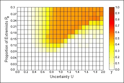
Figure 14. Heat-map over (u, pe) parameter-space showing mean value of y, with n = 300. 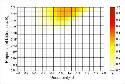
Figure 15. Heat-map over (u, pe) parameter-space showing mean value of y, with n = 1000. - 5.3
- We can see that as n increases the noise effects decrease as does the initial population instability (as shown by the vast area where y is consistently very close to 0). There are three reasons for this. The first is that zone of higher (> 0.3) mean-y values decreases in area as n increases; the second is that the 'noise' fluctuations due to small populations of extremists are lost; and the third is that the maximum y value across the whole parameter space is not as high when n is increased, although this seems mostly attributable to the decrease in noise.
- 5.4
- From this, we can see that the initial instability of the population is linked to initial uncertainty u and the proportion of extremist agents pe which admittedly was clear before but we now know that the significance of the role played by pe increases as n increases. When n is very large, u loses its significance because, if pe is not high, we will not create an initially unstable population. It should also be noted that this does not mean that with large values of n single extreme convergence will not occur; merely that the region of parameter space under which it is likely to occur becomes appreciably smaller. The reason that the area of instability shrinks is quite simple. As n grows, the number of moderate agents grows quicker than the number of extremist agents. Obviously this is due to the number of moderate agents constituting a larger proportion of the population than that of the extremists. In cases of bipolar and single extreme convergence, the influence of initially moderate agents on each other is very important, since it must be low enough overall to not restrain other moderate agents from forming a moderate opinion by the end of the experiment. As the number of moderate agents grows to large values, their influence can become increasingly strong and act as a stabilizer, even when uncertainties are very high. This is why although we may see the mean y-values reduce, that is largely due to the area of elevated mean-y values shifting upwards on the graph (i.e. linked with higher-pe regions of the parameter space), where the number of extremists is still large enough to exert an influence.
- 5.5
- It is curious to consider that while this influence may be true in a population that is fully connected, a population that has a distribution of connections that exhibits a high clustering coefficient could maybe become much more unstable if various clusters develop extreme opinions. It is of course possible that the much lower connectivity degree of the extremist agents may simply limit their influence and hence produce a more stable state. A serious examination of this would be beyond on the scope of this paper however, and so the next section will only briefly examine groups of populations.
Groups of Populations
- 6.1
- When the RA model is treated as a closed system, we obtain the results presented here, but what happens if we run several simulations simultaneously with occasional interaction between them? This would represent a more accurate picture of what happens in real life as it has been shown that social interaction is very often quite clustered. In a clustered model, we may find that although most groups can become centrally convergent there could be occasional instances of a single group demonstrating bipolar convergence or, more importantly for the arguments in this paper, single extreme convergence. If we could see occurrences whereby several of the groups converge centrally and a single or minority number of groups converge to a single extreme, then this could demonstrate the utility of such an extended model for succinctly describing the circumstances under which extremist groups may form in an otherwise rational and moderate population.
- 6.2
- However, after numerous experiments, our results suggest that unless the interaction between populations is minimal (to the extent that some populations may never interact, and those that do have less than a handful of interactions over the course of the tens of thousands of interactions that occur in total) each group will converge in a similar manner to the other groups, that is: the convergence is homogeneous. This implies that the structure of a system of groups (i.e., sub-populations) has a general influence over any single sub-population that is too strong to overcome and allow a breakaway result.
- 6.3
- While perhaps a superficially negative result, these results are encouraging for two reasons: first, a system of RA model sub-populations can be modeled by a single instance of the RA model, which saves any further complications; second, this has served to illuminate a missing piece of information in the RA model. In real human social systems, we know that clustering occurs naturally throughout society. We also know that a very small number of these clusters may become extreme (although a single cluster converging towards the bipolar situation is less common). We can see that, at least at this cursory examination, this does not occur under the original RA model's rules. Therefore, something must be modified in order to produce results that accurately reflect the nature of problem.
- 6.4
- Pursuing this avenue of research would involve changing the scope of the RA model from an examination of population-wide opinions to one that explores the effects that the clusters within the given population have on that population's opinion dynamics, and so is beyond the scope of this paper.
Further Work
- 7.1
- Having examined the role of low level interaction between agents and how that affects the dynamics of opinion formation among the population, the next logical step is to examine the role of external influences, such as propaganda. While there is already existing research into the role of propaganda on populace opinions, it has not been examined in the context of the BC or RA model. Extending the RA model to accommodate an approximation to propaganda could be sketched as follows: one agent may be selected at random and given extra interactions with other random agents or occasional one-way weakened interactions with all other agents. The interactions would have to be one-sided because in propaganda there is a few-to-many mapping where a relatively small number of individuals responsible for generating the propaganda do so in the expectation that it will influence the opinions of many more individuals in due course. A suitable tool for examining the success of the propaganda would be to compare the final population opinion against that of the "propagandist" agents. It would also be informative to explore how a single propagandist agent could affect the typical y-value patterns when initially primed with a particular given opinion.
Conclusion
- 8.1
- From the above experiments it is clear that the RA model has produced some interesting ideas and will continue to be a useful tool in the study of opinion dynamics, particularly in the examination of extremist opinion formation. It should also be clear however that the previously accepted view of the RA model's results was not entirely correct.
- 8.2
- There appear to be no conditions under which single extreme convergence will occur in the majority of the simulations. This is logical as the initial instability in the population that is required for single extreme convergence easily also allows for bipolar and central convergence.
- 8.3
- Furthermore it is clear that for single extreme convergence to occur there must be a large number of initially extreme agents, instead of a very low number. This too is logical; a large number of extremist agents will have a greater influence over the initially moderate agents compared to a lower proportion of extremists. This is still the case when it is noted that the group of extremist agents are competing against a larger group of opposite-extremist agents.
- 8.4
- While our results described here help to illuminate the dynamics of the RA model itself, there are some insights that can be taken from this work and applied to the real world. Now that we have seen that the influence of the extremist agents must be reasonably large in a highly uncertain population (particularly so in very large populations) we begin to understand at least one reason why in the whole of human history, relatively few populations have converged to have a bipolar or single extreme viewpoint (be it political, ideological or religious). It is also interesting to note that in instances where such convergences have occurred, the influence of the extremist viewpoint has been very strong combined with times when the average person would be considered highly uncertain or at the very least unsure and looking for ways to improve their circumstances. This certainly implies that the RA model offers a useful degree of realism in examining such population-level influences on opinion dynamics.
Appendix A: Source Code
-
Meadows' re-implementation of the Deffuant Model, in Java.
Agent.java
public class Agent {

	private double uncertainty;
	// Each agent is expected to interact (INTERACTIONS / N) * 2 times.  (Each interaction uses 2 agents.)
	// We double the expected length of history for safety.
	private double [] opinion;
	private int opinionCounter;

	public Agent(double o, double u) {
		this.opinion = new double[(RAModel.INTERACTIONS / RAModel.N) * 4];
		this.opinionCounter = 0;
		this.setOpinion(o);
		this.setUncertainty(u);
	} // Agent

	public double getUncertainty() {
		return this.uncertainty;
	} // getUncertainty
	public void setUncertainty(double u) {
		this.uncertainty = u;
	} // setUncertainty

	public double getOpinion() {
			return this.opinion[opinionCounter-1];
	} // getOpinion
	public double getOpinion(int i) {
		if (i < opinionCounter)
			return this.opinion[i];
		else
			return this.opinion[opinionCounter-1];
	} // getOpinion

	public void setOpinion(double o) {
		if (this.opinionCounter < this.opinion.length) {
			this.opinion[opinionCounter] = o;
			this.opinionCounter++;
		} else {
			System.out.println("Error:\tOpinion array not long enough.");
		}
	} // setOpinion

} // Agent
RAModel.java
import java.util.Random;
import java.io.*;

public class RAModel {

    public static final int SAMPLES = 50; // Number of repetitions at each parameter setting.
    public static final int INTERACTIONS = 40000; // Number of random agent interactions.

    public static final double OPINION_MIN = -1.0;
    public static final double OPINION_MAX = 1.0;

    public static final double EXTREMIST_OPINION_BOUNDARY = 0.8;
    public static final double EXTREMIST_UNCERTAINTY = 0.1;

    public static final double MU = 0.2; // How much agents affect each other.

    public static final int N = 200; // Number of agents
    public static final double Pe_MAX = 0.3; // Maximum proportion of Extremists.
    public static final double U_MAX = 2.0; // Maximum uncertainty.
    public static final int Pe_STEPS = 50; // Increments of Pe to test.
    public static final int U_STEPS = 10; // Increments of uncertainty to test.

    public static void main (String [] args) {

        Agent [] agent = new Agent[N];
        Random random = new Random();

        double [][] y = new double[Pe_STEPS][U_STEPS];

        double [] ySample = new double[SAMPLES];

        // Due to some hassle with the doubles, ints are used in the for loops with the doubles calculated immediately after.
        double Pe, U;
        for (int PeCounter = 0; PeCounter < Pe_STEPS; PeCounter++) {
        System.out.println("PeCounter " + PeCounter);
        Pe = (Pe_MAX / (double)Pe_STEPS) * (double)PeCounter;
        for(int UCounter = 0; UCounter < U_STEPS; UCounter++) {
        U = (U_MAX / (double)U_STEPS) * (double)UCounter;

        for (int sample = 0; sample < SAMPLES; sample++) {

            // Initialise agents (extremists then moderates).
            int numberOfExtremists = (int)(Pe * (double)N);
            if (numberOfExtremists % 2 == 1)
                numberOfExtremists++; // Maintain delta at 0 (p'+ == p'-).
            double randomOpinion;
            for (int i = 0; i < numberOfExtremists - 1; i = i + 2) {
                randomOpinion = (random.nextDouble() * (OPINION_MAX - EXTREMIST_OPINION_BOUNDARY)) + EXTREMIST_OPINION_BOUNDARY;
                agent[i] = new Agent(randomOpinion, EXTREMIST_UNCERTAINTY);
                randomOpinion = (random.nextDouble() * (OPINION_MAX - EXTREMIST_OPINION_BOUNDARY)) + EXTREMIST_OPINION_BOUNDARY;
                agent[i+1] = new Agent(-randomOpinion, EXTREMIST_UNCERTAINTY);
            }
            for (int i = numberOfExtremists; i < N; i++) {
                randomOpinion = (random.nextDouble() * (EXTREMIST_OPINION_BOUNDARY * 2)) - EXTREMIST_OPINION_BOUNDARY;
                agent[i] = new Agent(randomOpinion, U);
            }

            // Agents interact.
            for (int interaction = 0; interaction < INTERACTIONS; interaction++) {

                // Choose 2 random agents.
                int agenti, agentj;
                agenti = agentj = random.nextInt(N);
                do {
                    agenti = random.nextInt(N);
                } while (agenti == agentj);

                // Interact!
                double Xi, Xj, Ui, Uj;
                Xi = agent[agenti].getOpinion();
                Xj = agent[agentj].getOpinion();
                Ui = agent[agenti].getUncertainty();
                Uj = agent[agentj].getUncertainty();

                double Hji = Math.min(Xj + Uj, Xi + Ui) - Math.max(Xj - Uj, Xi - Ui);
                double Hij = Math.min(Xi + Ui, Xj + Uj) - Math.max(Xi - Ui, Xj - Uj);

                double RAji = (Hji / Uj) - 1.0;
                double RAij = (Hij / Ui) - 1.0;

                // Update
                if (Hji > Uj) {
                    agent[agenti].setOpinion( Xi + (MU * RAji * (Xj - Xi)) );
                    agent[agenti].setUncertainty( Ui + (MU * RAji * (Uj - Ui)) );
                } else {
                    agent[agenti].setOpinion(Xi); // For history.
                }
                if (Hij > Ui) {
                    agent[agentj].setOpinion( Xj + (MU * RAij * (Xi - Xj)) );
                    agent[agentj].setUncertainty( Uj + (MU * RAij * (Ui - Uj)) );
                } else {
                    agent[agentj].setOpinion(Xj); // For history.
                }
            } // interaction for loop end.

            // Calculate y.
            int newPositiveExtremists = 0;
            int newNegativeExtremists = 0;
            for (int i = numberOfExtremists; i < N; i++) { // Don't count original extremists.
                if (agent[i].getOpinion() > EXTREMIST_OPINION_BOUNDARY)
                    newPositiveExtremists++;
                if (agent[i].getOpinion() < -EXTREMIST_OPINION_BOUNDARY)
                    newNegativeExtremists++;
            }
            double pplus = (double)newPositiveExtremists / (double)(N - numberOfExtremists);
            double pminus = (double)newNegativeExtremists / (double)(N - numberOfExtremists);
            ySample[sample] = (pplus * pplus) + (pminus * pminus);

        } // sample for loop end.

            // Calculate and save average y for those parameters.
            double result = 0;
            for (int i = 0; i < ySample.length; i++)
                result += ySample[i];
            y[PeCounter][UCounter] = result / (double)SAMPLES;

        } // U for loop end.
        } // Pe for loop end.

        // Output results.
        try {
            FileWriter file = new FileWriter("results.txt");
            BufferedWriter buffer = new BufferedWriter(file);

            // Format and output data.
            // Pe \ Uncertainty 0.00 0.01 0.02 ...
            // 0.00                 x    x    x
            // 0.01                 x    x    x
            // 0.02                 x    x    x
            // ...
            for (U = 0.0; U < U_MAX; U = U + (U_MAX / (double)U_STEPS))
                buffer.write("\t" + ((Double)U).toString());
            int pe = 0;
            for (Pe = 0.0; Pe < Pe_MAX; Pe = Pe + (Pe_MAX / (double)Pe_STEPS)) {
                buffer.newLine();
                buffer.write( ((Double)Pe).toString() );
                for (int u = 0; u < y[pe].length; u++) {
                    buffer.write("\t" + ((Double)y[pe][u]).toString());
                }
                pe++;
            }

            buffer.close();
        } catch (IOException e) {
            System.out.println("Error:\tFile writing failed");
        }
    } // main
} // RAModel
Cliff's re-implementation of the Deffuant Model, in Python.
# a very simple implementation of Relative Agreement,
# aimed just at replicating Figure 9

import random
from math import sqrt

#range of uncertainty (U) values for moderate agents
u_min = 0.2
u_max = 2.0
#number of steps this u-range is divided into
u_steps = 19 #this was 19 in the original Fig 9

#range of global proportion of extremists (pe)
pe_min = 0.025
pe_max = 0.3
#number of steps the pe-range is divided into
pe_steps = 12 #this was 12 in the original Fig 9

#number of iid repetitions of the simulation at each (u,pe) point
sims_per_point = 50

#number of runs to dump as timeseries of opinion for each agent at each (u,pe)
n_dumps = 0

#opinion values
Max_Op = 1.0
Min_Op = -1.0

#population size
N = 200

#expected number of iterations per individual
n_iter = 250

#intensity of interactions
mu = 0.2

#extremism uncertainty
u_e = 0.1

#DC introduced this parameter:
#how close does the opinion value have to be to one of the extremes to count as extreme?
extreme_distance = 0.2

Min_mod_op=Min_Op+extreme_distance
Max_mod_op=Max_Op-extreme_distance

#calculate y value for a given u, pe pair
def calc_y(u, pe, dump, dumpid):

    if(dump>0):
        # write population values to file on this run
        filename='RA'+"_%2.3f"%u+"_%2.3f"%pe+"_%2d"%dumpid+'.csv'
        outfile=open(filename,'w')


    # generate initial population of individuals
    pop=[]
    for i in range(N):
        Op=Min_mod_op+(random.random()*(Max_mod_op-Min_mod_op))
        #pop structure is [opinion,certainty,start_opinion,n_iterations]
        pop.append([Op,u,"moderate",0])


    # use pe to determine number of extremists (and hence number of moderates)
    n_extremists=pe*N
    N_P_plus=int(0.5+(n_extremists/2.0))
    #assume symmetric plus/minus
    N_P_minus=N_P_plus
    n_moderate=N-(N_P_plus+N_P_minus)

    # create extremists: Max then Min
    for i in range(N_P_plus):
        pop[i][0]=Max_Op-(random.random()*extreme_distance)
        pop[i][1]=u_e
        pop[i][2]="extreme"

    for i in range(N_P_minus):
        pop[N_P_plus+i][0]=Min_Op+(random.random()*extreme_distance)
        pop[N_P_plus+i][1]=u_e
        pop[N_P_plus+i][2]="extreme"


    # this is the main experiment loop
    for iter in range(n_iter):

        # write the line of agent opinions for this iteration
        if(dump>0):
            outstr=""
            for i in range(N):
                if(i<(n-1)):
                    outstr+="%2.3f"%pop[i][0]+", "
                else:
                    outstr+="%2.3f"%pop[i][0]+"\n"
            outfile.write(outstr)


        #now do n updates

        for i in range(n):

            # randomly pick an individual to be influenced
            agent=random.randint(0,N-1)

            # randomly pick a different individual to be the influencer
            influencer=agent
            while(influencer==agent):
                influencer=random.randint(0,N-1)

            # allow them to interact and possibly alter opinions
            # switching to variable names used by deffuant et al
            x_j=pop[agent][0]
            u_j=pop[agent][1]
            x_i=pop[influencer][0]
            u_i=pop[influencer][1]
            h_ij=min(x_i+u_i, x_j+u_j) - max(x_i-u_i, x_j-u_j)
            if(h_ij>u_i):
                relagree=(h_ij/u_i)-1
                delta_x_j=mu*relagree*(x_i-x_j)
                delta_u_j=mu*relagree*(u_i-u_j)
                pop[agent][0]=x_j+delta_x_j
                pop[agent][1]=u_j+delta_u_j
                # print "influence! dx, du=",delta_x_j,delta_u_j

            # update the counts
            pop[agent][3]=pop[agent][3]+1
            pop[influencer][3]=pop[influencer][3]+1


    # now do the post-experiment analysis
    # compare current opinion and initial opinion
    p_prime_plus_count=0
    p_prime_minus_count=0

    for i in range(N):

        # increment p_prime_plus_count if this is a moderate that went +ve extreme
        if((pop[i][2]=="moderate")&((Max_Op-pop[i][0])<=extreme_distance)):
            p_prime_plus_count+=1;

        # increment p_prime_minus_count if this is a moderate that went -ve extreme
        if((pop[i][2]=="moderate")&((pop[i][0]-Min_Op)<=extreme_distance)):
            p_prime_minus_count+=1


    p_prime_plus=p_prime_plus_count/float(n_moderate)
    p_prime_minus=p_prime_minus_count/float(n_moderate)

    y=(p_prime_plus*p_prime_plus)+(p_prime_minus*p_prime_minus)
    print "y=",y

    #write the number of interactions each agent has had
    if(dump>0):
        outstr="\n"
        for i in range(N):
            if(i<(n-1)):
                outstr+="%3d"%pop[i][3]+", "
            else:
                outstr+="%3d"%pop[i][3]+"\n"
                outfile.write(outstr)

        outfile.close()

    return y


#calculate min, max, avg & stdev of y value for a given u, pe pair over n trials

def calc_y_stats(u,pe):
    y_max=-10.0
    y_min=10.0
    y_sum=0.0
    y_sumsq=0.0
    for sim in range(sims_per_point):
        if(sim<n_dumps):
            dump=1
        else:
            dump=0
        y=calc_y(u, pe, dump, sim)
        y_sum=y_sum+y
        y_sumsq=y_sumsq+(y*y)
        if(y>y_max):
            y_max=y
        if(y<y_min):
            y_min=y
    y_avg=y_sum/sims_per_point
    y_sd=sqrt((y_sumsq/sims_per_point)-(y_avg*y_avg))
    return (y_max, y_min, y_avg, y_sd)


#main: calc avg + sd for y at each (u,pe) point

u_delta=(u_max-u_min)/(u_steps-1)
pe_delta=(pe_max-pe_min)/(pe_steps-1)
mindata=[]
maxdata=[]
avgdata=[]
sdvdata=[]

for u_i in range(u_steps):
    u=u_min+(u_i*u_delta)
    minrow=[]
    maxrow=[]
    avgrow=[]
    sdvrow=[]
    for pe_i in range(pe_steps):
        pe=pe_min+(pe_i*pe_delta)
        y_stats=calc_y_stats(u, pe)
        print (u_i, pe_i), (u, pe), y_stats
        minrow.append(y_stats[1])
        maxrow.append(y_stats[0])
        avgrow.append(y_stats[2])
        sdvrow.append(y_stats[3])
    mindata.append(minrow)
    maxdata.append(maxrow)
    avgdata.append(avgrow)
    sdvdata.append(sdvrow)

#print it all out
outfile=open('RAout_min.csv','w')
for u_i in range(u_steps):
    outstr=""
    for pe_i in range(pe_steps):
        if(pe_i<(pe_steps-1)):
           outstr+="%2.4f"%mindata[u_i][pe_i]+", "
        else:
           outstr+="%2.4f"%mindata[u_i][pe_i]+"\n"

    outfile.write(outstr)
    print outstr
outfile.close()

#print it all out
outfile=open('RAout_max.csv','w')
for u_i in range(u_steps):
    outstr=""
    for pe_i in range(pe_steps):
        if(pe_i<(pe_steps-1)):
           outstr+="%2.4f"%maxdata[u_i][pe_i]+", "
        else:
           outstr+="%2.4f"%maxdata[u_i][pe_i]+"\n"

    outfile.write(outstr)
    print outstr
outfile.close()

#print it all out
outfile=open('RAout_avg.csv','w')
for u_i in range(u_steps):
    outstr=""
    for pe_i in range(pe_steps):
        if(pe_i<(pe_steps-1)):
           outstr+="%2.4f"%avgdata[u_i][pe_i]+", "
        else:
           outstr+="%2.4f"%avgdata[u_i][pe_i]+"\n"

    outfile.write(outstr)
    print outstr
outfile.close()

#print it all out
outfile=open('RAout_stdev.csv','w')
for u_i in range(u_steps):
    outstr=""
    for pe_i in range(pe_steps):
        if(pe_i<(pe_steps-1)):
           outstr+="%2.4f"%sdvdata[u_i][pe_i]+", "
        else:
           outstr+="%2.4f"%sdvdata[u_i][pe_i]+"\n"

    outfile.write(outstr)
    print outstr
outfile.close()
References
-
CHATTERJEE, S. and Seneta, E. (1977). Towards Consensus: Some Convergence Theorems on Repeated Averaging. Journal of Applied Probability , 14(1): 88-97. [doi:10.2307/3213262]
DE GROOT, M. (1974). Reaching a Consensus. Journal of the American Statistical Association 69 (345): 118-121. [doi:10.1080/01621459.1974.10480137]
DEFFUANT, G., Neau, D. and Amblard, F. (2000). Mixing beliefs among interacting agents. Advances in Complex Systems , 3:87-98. [doi:10.1142/S0219525900000078]
DEFFUANT, G., Amblard, F., Weisbuch, G. and Faure, T. (2002). How can extremism prevail? A study based on the relative agreement interaction model. Journal of Artificial Societies and Social Simulation , 5(4): 1 https://www.jasss.org/5/4/1.html.
DEFFUANT, G. (2006). Comparing Extremism Propagation Patterns in Continuous Opinion Models. Journal of Artificial Societies and Social Simulation , 9(3):8 https://www.jasss.org/9/3/8.html.
FRIEDKIN, N. (1999). Choice Shift and Group Polarization. American Sociological Review 64(6): 856-875 . [doi:10.2307/2657407]
HEGSELMANN, R. and Krause, U. (2002). Opinion dynamics and bounded confidence: models, analysis and simulation. Journal of Artificial Societies and Social Simulation , 5(3) 2 https://www.jasss.org/5/3/2.html
KRAUSE, U. (2000). A Discrete Nonlinear and Non-Autonomous Model of Consensus Formation. Communications in difference equations: Proceedings of the Fourth International Conference on Difference Equations, Poznan, Poland, August 27-31, 1998, 227-236. [doi:10.1201/b16999-21]
LORENZ, J. (2005). A stabilization theorem for dynamics of continuous opinions. Physica A: Statistical Mechanics and its Applications , 355(1). [doi:10.1016/j.physa.2005.02.086]
LORENZ, J. (2007). Continuous Opinion Dynamics under Bounded Confidence: A Survey. International Journal of Modern Physics C 18:1-20. [doi:10.1142/S0129183107011789]