
Segismundo S. Izquierdo, Luis R. Izquierdo and Nicholas M. Gotts (2008)
Reinforcement Learning Dynamics in Social Dilemmas
Journal of Artificial Societies and Social Simulation
vol. 11, no. 2 1
<https://www.jasss.org/11/2/1.html>
For information about citing this article, click here
Received: 21-Jan-2007 Accepted: 17-May-2007 Published: 31-Mar-2008

 Abstract
Of several responses made to the same situation those which are accompanied or closely followed by satisfaction to the animal will, other things being equal, be more firmly connected with the situation, so that, when it recurs, they will be more likely to recur; those which are accompanied or closely followed by discomfort to the animal will, other things being equal, have their connections to the situation weakened, so that, when it recurs, they will be less likely to occur. The greater the satisfaction or discomfort, the greater the strengthening or weakening of the bond. (Thorndike 1911, p. 244)
|
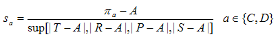
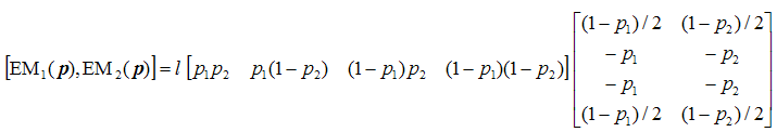
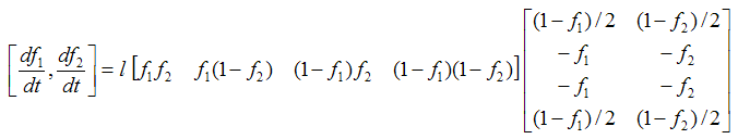
where πa is the payoff obtained having selected action a, A is the player's aspiration level[1], and T , R , P , S are the possible payoffs the player might receive, as explained above. Hence the stimulus is always a number in the interval [-1, 1]. Secondly, having calculated their stimulus sai , each player i updates her probability pai of undertaking the selected action a as follows (where every variable is indexed in i):
|
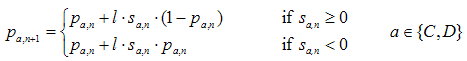
where pa,n is the probability of undertaking action a in time-step n, sa,n is the stimulus experienced after having selected action a in time-step n, and l is the learning rate (0 < l < 1). Thus the higher the stimulus (or the learning rate), the larger the change in probability. The updated probability for the action not selected derives from the constraint that probabilities must add up to one.
|
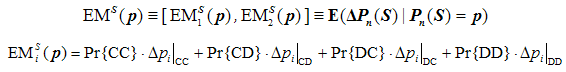
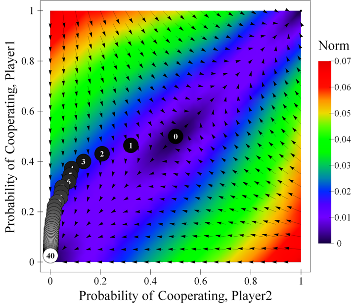
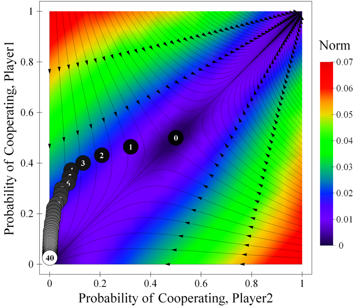
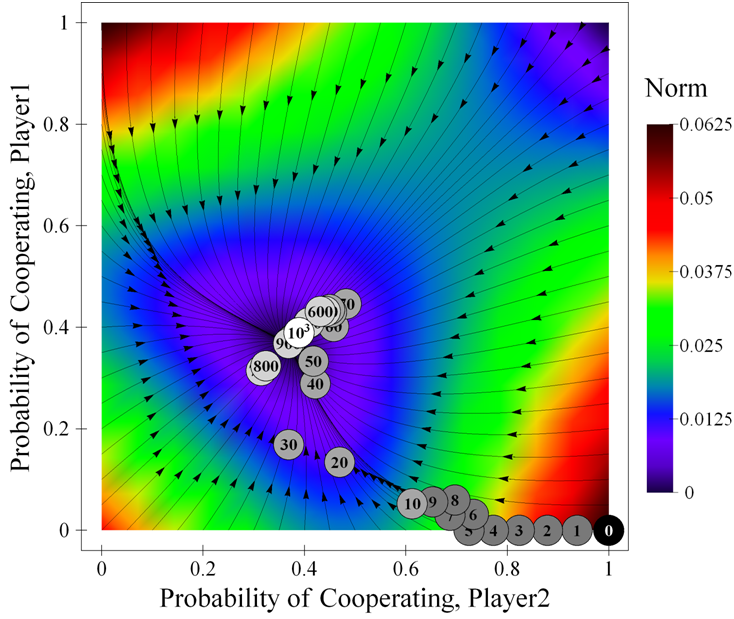
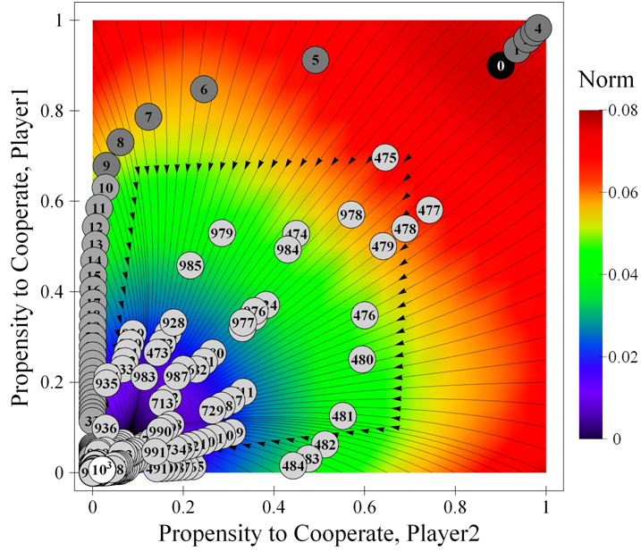
where {CC, CD, DC, DD} represent the four possible outcomes that may occur. Note that in general the expected change will not reflect the actual change in a simulation run, and to make this explicit we have included the trace of a simulation run starting in state [ 0.5 , 0.5 ] in figure 1. The expected change —represented by the arrows in figure 1— is calculated considering the four possible changes that could occur (see equation above), whereas the actual change in a simulation run —represented by the numbered balls in figure 1— is only one of the four possible changes (e.g. Δpi|CC, if both agents happen to cooperate).
|
| Figure 1. Expected motion of the system in a Stag Hunt game parameterised as [ 3 , 4 , 1 , 0 | 0.5 | 0.5 ]2, together with a sample simulation run (40 iterations). The arrows represent the expected motion for various states of the system; the numbered balls show the state of the system after the indicated number of iterations in the sample run. The background is coloured using the norm of the expected motion. For any other learning rate the size of the arrows would vary but their direction would be preserved. The source code used to create this figure is available in the Supporting Material. |
|
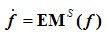
(1) |
or, equivalently,
|
|
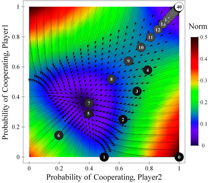
| Figure 2. Trajectories in the phase plane of the differential equation corresponding to a Stag Hunt game parameterised as [ 3 , 4 , 1 , 0 | 0.5 | 0.5 ]2, together with a sample simulation run (40 iterations). The background is coloured using the norm of the expected motion. The source code used to create this figure is available in the Supporting Material. |
|
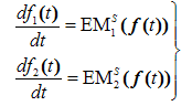
And the associated differential equation is
|
|
| Figure 3. Trajectories in the phase plane of the differential equation corresponding to the Prisoner's Dilemma game parameterised as [ 4 , 3 , 1 , 0 | 2 | l ]2, together with a sample simulation run ( l = 2-4 ). This system has an SCE at [ 0.37 , 0.37 ]. The background is coloured using the norm of the expected motion. The source code used to create this figure is available in the Supporting Material. |
|
| Figure 4. Expected motion of the system in a Prisoner's Dilemma game parameterised as [ 4 , 3 , 1 , 0 | 2 | 0.5 ]2, with a sample simulation run. The background is coloured using the norm of the expected motion. The source code used to create this figure is available in the Supporting Material. |
|
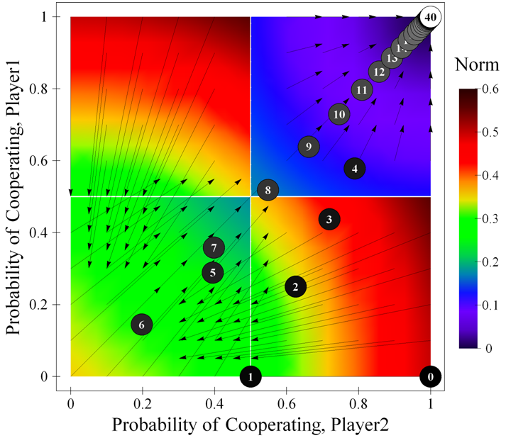
| Figure 5. Figure showing the most likely movements at some states of the system in a Prisoner's Dilemma game parameterised as [ 4 , 3 , 1 , 0 | 2 | 0.5 ]2, with a sample simulation run. The background is coloured using the norm of the expected motion. The source code used to create this figure is available in the Supporting Material. |
|
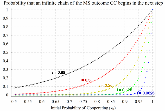
| Figure 6. Probability of starting an infinite chain of the Mutually Satisfactory (MS) outcome CC in a Prisoner's Dilemma game parameterised as [ 4 , 3 , 1 , 0 | 2 | l ]2. The 5 different (coloured) series correspond to different learning rates l. The variable x0, represented in the horizontal axis, is the initial probability of cooperating for both players. The source code used to create this figure is available in the Supporting Material. |
By the ultralong run, we mean a period of time long enough for the asymptotic distribution to be a good description of the behavior of the system. The long run refers to the time span needed for the system to reach the vicinity of the first equilibrium in whose neighborhood it will linger for some time. We speak of the medium run as the time intermediate between the short run [i.e. initial conditions] and the long run, during which the adjustment to equilibrium is occurring. (Binmore, Samuelson and Vaughan 1995, p. 10)
|
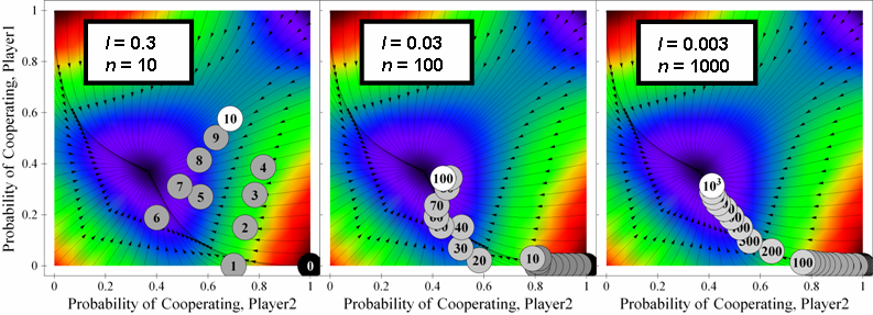
| Figure 7. Three sample runs of a system parameterised as [ 4 , 3 , 1 , 0 | 2 | l ]2. for different values of n and l. The product n·l is the same for the three simulations; therefore, for low values of l, the state of the system at the end of the simulations tends to concentrate around the same point. The source code used to create this figure is available in the Supporting Material. |
|
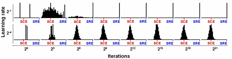
| Figure 8. Histograms representing the probability of cooperating for one player (both players' probabilities are identical) after n iterations for different learning rates l in a Prisoner's Dilemma game parameterised as [ 4 , 3 , 1 , 0 | 2 | l ]2, each calculated over 1,000 simulation runs. The initial probability for both players is 0.5. The source code used to create this figure is available in the Supporting Material. |
|
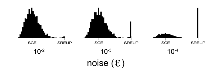
| Figure 9. Histograms representing the propensity to cooperate for one player (both players' propensities are identical) after 1,000,000 iterations (when the distribution is stable) for different levels of noise (εi = ε) in a Prisoner's Dilemma game parameterised as [ 4 , 3 , 1 , 0 | 2 | 0.25 ]2. Each histogram has been calculated over 1,000 simulation runs. The source code used to create this figure is available in the Supporting Material. |
|
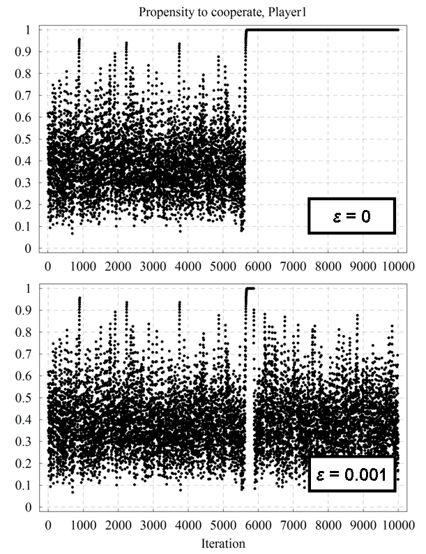
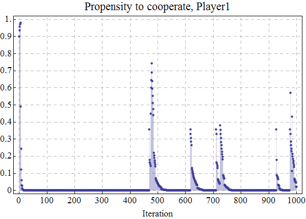
| Figure 10. A representative time series of player 1's propensity to cooperate over time for the Prisoner's Dilemma game parameterised as [ 4 , 3 , 1 , 0 | 2 | 0.5 ]2 with initial conditions [ x0 , x0 ] = [ 0.5 , 0.5 ], both without noise (top) and with a noise level εi = 10-3 (bottom). The source code used to create this figure is available in the Supporting Material. |
|
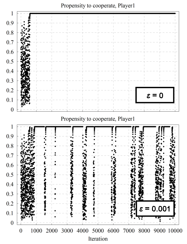
| Figure 11. A representative time series of player 1's propensity to cooperate over time for the Prisoner's Dilemma game parameterised as [ 4 , 3 , 1 , 0 | 2 | 0.25 ]2 with initial conditions [ x0 , x0 ] = [ 0.5 , 0.5 ], both without noise (top) and with a noise level εi = 10-3 (bottom). The source code used to create this figure is available in the Supporting Material. |
|
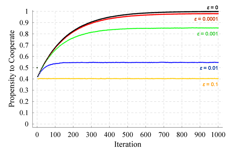
| Figure 12. Evolution of the average probability / propensity to cooperate of one of the players in a Prisoner's Dilemma game parameterised as [ 4 , 3 , 1 , 0 | 2 | 0.5 ]2 with initial state [ 0.5 , 0.5 ], for different levels of noise (εi = ε). Each series has been calculated averaging over 100,000 simulation runs. The standard error of the represented averages is lower than 3·10-3 in every case. The source code used to create this figure is available in the Supporting Material. |
|
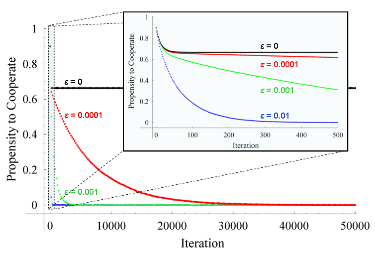
| Figure 13. Evolution of the average probability / propensity to cooperate of one of the players in a Prisoner's Dilemma game parameterised as [ 4 , 3 , 1 , 0 | 0.5 | 0.5 ]2 with initial state [ 0.9 , 0.9 ], for different levels of noise (εi = ε). Each series has been calculated averaging over 10,000 simulation runs. The inset graph is a magnification of the first 500 iterations. The standard error of the represented averages is lower than 0.01 in every case. The source code used to create this figure is available in the Supporting Material. |
|
| Figure 14. One representative run of the system parameterised as [ 4 , 3 , 1 , 0 | 0.5 | 0.5 ]2 with initial state [ 0.9 , 0.9 ], and noise εi = ε = 0.1. This figure shows the evolution of the system in the phase plane of propensities to cooperate, while figure 15 below shows the evolution of player 1's propensity to cooperate over time for the same simulation run. The background is coloured using the norm of the expected motion. The source code used to create this figure is available in the Supporting Material. |
|
| Figure 15. Time series of player 1's propensity to cooperate over time for the same simulation run displayed in figure 14. The source code used to create this figure is available in the Supporting Material. |
2 The concept of SRE is extensively used by Macy and Flache but we have not found a clear definition in their papers (Macy and Flache 2002; Flache and Macy 2002). Sometimes their use of the word SRE seems to follow our definition (e.g. Macy and Flache 2002, p. 7231), but often it seems to denote a mutually satisfactory outcome (e.g. Macy and Flache 2002, p. 7231) or an infinite sequence of such outcomes (e.g. Macy and Flache 2002, p. 7232).
3 The specification of the model is such that probabilities cannot reach the extreme values of 0 or 1 starting from any other intermediate value. Therefore if we find a simulation run that has actually ended up in the lock-in state [ 1 , 1 ] starting from any other state, we know for sure that such simulation run did not follow the specifications of the model (e.g. perhaps because of floating-point errors). For a detailed analysis of the effects of floating point errors in computer simulations, with applications to this model in particular, see Izquierdo and Polhill (2006), Polhill and Izquierdo (2005), Polhill et al. (2006), Polhill et al. (2005).
4 Maximin is the largest possible payoff players can guarantee themselves. In the three 2×2 social dilemmas maximini = max(Si, Pi).
5 Recall that each player's aspiration level is assumed to be different from every payoff the player may receive.
6 Excluded here is the trivial case where the initial state is an SRE.
7 We exclude here the meaningless case where the payoffs for some player are all the same and equal to her aspiration (Ti = Ri = Pi = Si = Ai for some i).
|
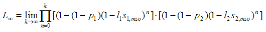
where li denotes player i's learning rate, and si,mso denotes player i's stimulus after the mutually satisfactory outcome mso. The following result can be used to estimate L∞ with arbitrary precision:
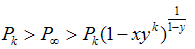
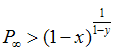
LetThis result is based on the bound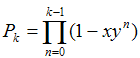
and let.
Then, for x, y in the interval (0, 1),
BENDOR J, Mookherjee D and Ray D (2001b) Reinforcement Learning in Repeated Interaction Games. Advances in Theoretical Economics 1(1), Article 3.
BINMORE K and Samuelson L (1993) An Economist's Perspective on the Evolution of Norms. Journal of Institutional and Theoretical Economics 150, 45-63.
BINMORE K, Samuelson L and Vaughan R (1995) Musical Chairs: Modeling Noisy Evolution. Games and Economic Behavior 11(1), 1-35.
BÖRGERS T and Sarin R (1997) Learning through Reinforcement and Replicator Dynamics. Journal of Economic Theory 77(1), 1-14.
BUSH R and Mosteller F (1955) Stochastic Models of Learning. John Wiliey & Son, New York.
CAMERER C F (2003) Behavioral Game Theory: Experiments in Strategic Interaction. Russell Sage Foundation, New York.
CASTELLANO C, Marsili M, and Vespignani A (2000) Nonequilibrium phase transition in a model for social influence. Physical Review Letters, 85(16), pp. 3536-3539.
CHEN Y and Tang F (1998) Learning and Incentive-Compatible Mechanisms for Public Goods Provision: An Experimental Study. Journal of Political Economy 106(3), 633-662.
CROSS J G (1973) A Stochastic Learning Model of Economic Behavior. Quartertly Journal of Economics 87(2), 239-266.
DAWES R M (1980) Social Dilemmas. Annual Review of Psychology 31, 169-93.
DUFFY J (2006) Agent-Based Models and Human Subject Experiments. In: Tesfatsion, L., Judd, K. L. (Eds.), Handbook of Computational Economics II: Agent-Based Computational Economics, chapter 19, 949-1011. Amsterdam: Elsevier.
EDWARDS M, Huet S, Goreaud F and Deffuant G (2003) Comparing an individual-based model of behaviour diffusion with its mean field aggregate approximation. Journal of Artificial Societies and Social Simulation 6(4)9. https://www.jasss.org/6/4/9.html.
ELLISON G (2000) Basins of Attraction, Long-Run Stochastic Stability, and the Speed of Step-by-Step Evolution. Review of Economic Studies 67, 17-45.
EREV I and Roth A E (1998) Predicting How People Play Games: Reinforcement Learning in Experimental Games with Unique, Mixed Strategy Equilibria. American Economic Review 88(4), 848-881.
EREV I, Bereby-Meyer Y and Roth A E (1999) The effect of adding a constant to all payoffs: experimental investigation, and implications for reinforcement learning models. Journal of Economic Behavior and Organization 39(1), 111-128.
EREV I and Roth A E (2001) Simple Reinforcement Learning Models and Reciprocation in the Prisoner's Dilemma Game. In: Gigerenzer, G., Selten, R. (Eds.), Bounded rationality: The Adaptive Toolbox. MIT Press, Cambridge.
FLACHE A and Macy M W (2002) Stochastic Collusion and the Power Law of Learning. Journal of Conflict Resolution 46(5), 629-653.
FOSTER D and Young H P (1990) Stochastic Evolutionary Game Dynamics. Theoretical Population Biology 38, 219-232.
GALÁN J M and Izquierdo L R (2005) Appearances Can Be Deceiving: Lessons Learned Re-Implementing Axelrod's 'Evolutionary Approach to Norms'. Journal of Artificial Societies and Social Simulation 8(3)2. https://www.jasss.org/8/3/2.html.
HUET S, Edwards M, and Deffuant G (2007) Taking into Account the Variations of Neighbourhood Sizes in the Mean-Field Approximation of the Threshold Model on a Random Network. Journal of Artificial Societies and Social Simulation 10(1)10. https://www.jasss.org/10/1/10.html.
IZQUIERDO L R, Polhill J G (2006). Is Your Model Susceptible to Floating-Point Errors?. Journal of Artificial Societies and Social Simulation 9(4)4. https://www.jasss.org/9/4/4.html.
IZQUIERDO L R, Izquierdo S S, Gotts N M and Polhill J G (2007) Transient and Asymptotic Dynamics of Reinforcement Learning in Games. Games and Economic Behavior 61(2), pp. 259-276.
KARANDIKAR R, Mookherjee D, Ray D and Vega-Redondo F (1998) Evolving Aspirations and Cooperation. Journal of Economic Theory 80(2), 292-331.
KIM Y (1999) Satisficing and optimality in 2×2 common interest games. Economic Theory 13(2), 365-375.
MACY M W (1989) Walking out of social traps: A stochastic learning model for the Prisoner's Dilemma. Rationality and Society 1(2), 197-219.
MACY M W (1991) Learning to cooperate: Stochastic and tacit collusion in social exchange. The American Journal of Sociology 97(3), 808-843.
MACY M W and Flache A (2002) Learning Dynamics in Social Dilemmas. Proceedings of the National Academy of Sciences USA 99(3), 7229-7236.
MCALLISTER P H (1991) Adaptive approaches to stochastic programming. Annals of Operations Research 30(1), 45-62.
MOHLER R R (1991) Nonlinear Systems, Volume I: Dynamics and Control. Prentice Hall, Englewood Cliffs.
MOOKHERJEE D and Sopher B (1994) Learning Behavior in an Experimental Matching Pennies Game. Games and Economic Behavior 7(1), 62-91.
MOOKHERJEE D and Sopher B (1997) Learning and Decision Costs in Experimental Constant Sum Games. Games and Economic Behavior 19(1), 97-132
NORMAN M F(1968) Some Convergence Theorems for Stochastic Learning Models with Distance Diminishing Operators. Journal of Mathematical Psychology 5(1), 61-101.
NORMAN M F(1972) Markov Processes and Learning Models. Academic Press, New York.
PALOMINO F and Vega-Redondo F (1999) Convergence of Aspirations and (partial) cooperation in the Prisoner's Dilemma. International Journal of Game Theory 28(4), 465-488.
PAZGAL A (1997) Satisficing Leads to Cooperation in Mutual Interests Games. International Journal of Game Theory 26(4), 439-453.
POLHILL J G and Izquierdo L R (2005) Lessons learned from converting the artificial stock market to interval arithmetic. Journal of Artificial Societies and Social Simulation 8(2) 2. https://www.jasss.org/8/2/2.html
POLHILL J G, Izquierdo L R, and Gotts N M (2005) The ghost in the model (and other effects of floating point arithmetic). Journal of Artificial Societies and Social Simulation 8(1) 5. https://www.jasss.org/8/1/5.html
POLHILL J G, Izquierdo L R, and Gotts N M (2006) What every agent based modeller should know about floating point arithmetic. Environmental Modelling and Software 21(3), 283-309.
ROTH A E and Erev I (1995) Learning in Extensive-Form Games: Experimental Data and Simple Dynamic Models in the Intermediate Term. Games and Economic Behavior 8(1), 164-212.
SELTEN R (1975) Re-examination of the Perfectness Concept for Equilibrium Points in Extensive Games. International Journal of Game Theory 4(1), 25-55.
THORNDIKE E L (1898) Animal Intelligence: An Experimental Study of the Associative Processes in Animals (Psychological Review, Monograph Supplements, No. 8). MacMillan, New York.
THORNDIKE E L (1911) Animal Intelligence. New York: The Macmillan Company.
WEIBULL J W (1995) Evolutionary Game Theory. Cambridge, MA: MIT Press.
YOUNG H P (1993) The evolution of conventions. Econometrica 61(1), 57-84
 Return to Contents of this issue
© Copyright Journal of Artificial Societies and Social Simulation, [2008]