©Copyright JASSS

JASSS logo ----

Stéphane Airiau, Sabyasachi Saha and Sandip Sen (2007)

Evolutionary Tournament-Based Comparison of Learning and Non-Learning Algorithms for Iterated Games

Journal of Artificial Societies and Social Simulation vol. 10, no. 3 7
<https://www.jasss.org/10/3/7.html>

For information about citing this article, click here

Received: 06-Dec-2005    Accepted: 09-Jun-2007    Published: 30-Jun-2007

PDF version


* Abstract

Evolutionary tournaments have been used effectively as a tool for comparing game-playing algorithms. For instance, in the late 1970's, Axelrod organized tournaments to compare algorithms for playing the iterated prisoner's dilemma (PD) game. These tournaments capture the dynamics in a population of agents that periodically adopt relatively successful algorithms in the environment. While these tournaments have provided us with a better understanding of the relative merits of algorithms for iterated PD, our understanding is less clear about algorithms for playing iterated versions of arbitrary single-stage games in an environment of heterogeneous agents. While the Nash equilibrium solution concept has been used to recommend using Nash equilibrium strategies for rational players playing general-sum games, learning algorithms like fictitious play may be preferred for playing against sub-rational players. In this paper, we study the relative performance of learning and non-learning algorithms in an evolutionary tournament where agents periodically adopt relatively successful algorithms in the population. The tournament is played over a testbed composed of all possible structurally distinct 2×2 conflicted games with ordinal payoffs: a baseline, neutral testbed for comparing algorithms. Before analyzing results from the evolutionary tournament, we discuss the testbed, our choice of representative learning and non-learning algorithms and relative rankings of these algorithms in a round-robin competition. The results from the tournament highlight the advantage of learning algorithms over players using static equilibrium strategies for repeated plays of arbitrary single-stage games. The results are likely to be of more benefit compared to work on static analysis of equilibrium strategies for choosing decision procedures for open, adapting agent society consisting of a variety of competitors.

Keywords:
Repeated Games, Evolution, Simulation

* Introduction

1.1
Learning and reasoning in single or multi-stage games has been an active area of research in multiagent systems (Banerjee, Sen, & Peng 2001;Bowling & Veloso 2001; Claus & Boutilier 1998; Greenwald & Hall 2003; Hu &Wellman 1998; Littman 1994, 2001; Littman & Stone 2001). In particular, iterative versions of single-stage bimatrix games have been used to evaluate learning algorithms by multiagent researchers. Particular games like the Prisoner's Dilemma (PD) have received widespread attention both in game theory (Axelrod 1985, 1987) and in multiagent systems (Sandholm & Crites 1995). The goals of multiagent learning research include the design of algorithms that converge to an equilibrium strategy and that play a best response to an opponent playing a stationary strategy (Bowling & Veloso 2002). Another goal is the prevention of the exploitation of learning algorithms (e.g., Bully (Littman & Stone 2001) tries to exploit any learning algorithm). A desirable property of learners is that they should not exhibit regret (Jafari et al. 2001;Bowling 2005). Solution concepts like Nash Equilibrium (NE) have been proposed as desired outcome for rational play. We refer to a player who always plays a Nash strategy as a Nash player. Playing a Nash strategy is not, in general, the best response to a sub-rational strategy. Against an unknown opponent, the use of a learning algorithm that adapts to the opponent algorithm can be preferable to playing a pre-determined static strategy.

1.2
Prior learning research has largely focused on one-on-one play. Our goal is to identify approaches, learning or otherwise (for example, using static equilibrium strategies), that will perform well in an open environment containing both rational and sub-rational algorithms, and when evaluated over an extensive range of challenging games. We believe that real-life open environments will include a large diversity of agent algorithms including rational and sub-rational, static and learning players. In particular, we study the evolution of a population of agents repeatedly participating in a round-robin competition involving a varied set of representative games and periodically adopting relatively successful algorithms, resulting in an evolutionary tournament. We believe that such evolutionary tournaments mimic real-life situations where users adapt their decision mechanism based on their observed performance in the environment. The results in this paper help us understand and predict the dynamics in the marketplace given realistic assumptions about initial algorithm distribution, stability of agent populations and selection schemes used by agents. The equilibrium reached via such a dynamic, evolutionary process provides better characterization of real-world environments composed of heterogeneous agents than static analysis of games to obtain rational equilibrium strategies. We believe that a study of such evolutionary equilibrium is more useful for selecting a preferred decision mechanism compared to static equilibrium analysis like Nash equilibrium. In such dynamic contexts, a preferred algorithm should be able to perform well over many situations and against many opponents, including itself, which ensures that the algorithm performs robustly in different heterogeneous agents populations.

1.3
To ensure a diversity of algorithms in the population, agents using representative learning and non-learning algorithms are used to form the initial population. At each generation of the evolutionary tournament, a round-robin competition is held where each agent plays against all other agents and itself on a neutral but extensive testbed of games: the testbed is composed of all possible conflicted two-action, two-player games with a total preference order over the four outcomes of the game [1]. This testbed represents a wide variety of situations, including often-studied games like PD, the chicken game, battle of the sexes, etc. There are other testbeds for arbitrary number of players, arbitrary number of actions (Nudelman et al 2004), but the class of conflicting two-action, two-player games provides a sufficiently rich environment for our purpose. Learners typically know only their own payoff matrices but are assumed to be able to observe opponent actions. We, however, allow players like the Nash player or Bully, to access the opponent's payoffs, which is necessary for the computation of their strategy. Lack of knowledge of opponent payoff is a more realistic assumption in an open environment. To compensate for the disadvantage given to these static players, several iterations are played for a given game, which gives the learning players an opportunity to adapt and respond effectively to the algorithm used by their opponent. We are interested not in the outcome of individual games, but in evaluating the performance of a set of algorithms over all games. Consequently in the iteration of the evolutionary tournament, the performance of an agent is measured by the cumulative payoff received over all iterations, games, and opponents. All the games and opponents are equally important in this metric. For a given pair of algorithms, some games may impact the score more than others, but we will not consider this level of detail in this paper. An agent selects the algorithm to use in the next generation of the evolutionary tournament with the knowledge of the performance and algorithms of all (or a subset of) the agents. Also, we are not attempting to construct an algorithm that would perform well in this environment. Our work is similar to Axelrod's work with a genetic algorithm in the context of the prisoners' dilemma tournament (Axelrod 1987). In our experiments, the algorithms remains fixed throughout the evolutionary process. Surviving algorithms from such evolutionary process are more robust and effective than extinct ones. Results from such tournaments show that learning algorithms are more robust than non-learning algorithms and are preferable for such dynamic, heterogeneous populations.

1.4
In Section 2, we present the evolutionary tournament structure with the testbed, the setting of the round-robin competition used during each generation of the evolutionary tournament and the selection mechanism used to determine the distribution of the algorithms in the successive generations. In Section 3, we present the algorithms that are present in the initial population. Section 4 contains experimental results: first we discuss results from a round-robin competition with one player per algorithm, and then we present results from the evolutionary tournament with different selection mechanisms. Section 5 summarizes the main findings of this research and presents future research possibilities.

* Tournament Structure

2.1
In this section, we describe the evolutionary tournament structure. We start with the description of the matrices that will be used in the round-robin competition in each generation along with the performance metric. Finally, we introduce the evolutionary tournament and present the different selection mechanisms that determine the algorithm distribution in the population for successive generations.

Testbed: Structurally distinct 2×2 conflicted games with ordinal payoffs

2.2
We consider a subset of two-player, two-action games where agents have a total preference order over the four possible outcomes. We use one of the numbers 1, 2, 3, and 4 as the preference of an agent for an outcome of the 2×2 matrix, 4 being the most preferred. Though these numbers correspond to ordinal payoffs, we treat them as cardinal payoffs. We do not consider games where both agents have the highest preference for the same outcome. These games are trivial to solve since no agent has any incentive to play anything but the action yielding the most preferred outcome. The testbed contains only situation where a conflict exists and therefore is made of 57 structurally distinct (i.e., no two games are identical by renaming the actions or the players) 2×2 conflict games as described in Brams (1994).

2.3
Nash equilibrium has been proposed as a solution concept for general-sum games. Strategies constitute a Nash Equilibrium when no player can benefit by changing its strategy while the other players retain their current strategies. More formally, for a two-player game with payoffs given by R and C, a pure-strategy Nash Equilibrium is a pair of actions (r*,c*) such that R(r*,c*) ≥ R(r, c*) ∀r and C(r*,c*) ≥ C(r*,c) ∀c. In a Nash equilibrium, the action chosen by each player is the best response to the opponent's current strategy and no player in this game has any incentive for unilateral deviation from its current strategy. A general-sum bimatrix game may not have any pure-strategy Nash Equilibrium. A mixed-strategy Nash Equilibrium is a pair of probability vectors (π1*, π2*) over the respective action space of each player such that ∀π1, tπ*1·R·π*2tπ1·R·π*2 and ∀π2, tπ*1·C·π2*tπ*1·C·π2. Every finite bimatrix game has at least one mixed-strategy Nash Equilibrium. Another relevant concept is Pareto optimality: an outcome is Pareto optimal if no player can improve its payoff without decreasing the payoff of any other player. If a single player deviates from a Pareto optimal equilibrium to increase its payoff, the payoff of another player will decrease.

2.4
The testbed of 57 matrices represents all the distinct conflicted games with ordinal payoffs. 51 of these games have a unique Nash equilibrium (9 of these games have a mixed strategy equilibrium and 42 have pure strategy equilibrium), the remaining 6 have multiple equilibria (two pure and a mixed strategy). Of the 42 games that have a unique pure strategy Nash equilibrium, in 4 games the Nash equilibrium is not Pareto-optimal.

2.5
A given algorithm might perform well against some opponents in particular games, i.e., an algorithm might be more suitable in some situations than others. A robust solution, however, should do well in a wide variety of games against a diverse set of opponents. We can expect the winner of a tournament between a diverse set of algorithms and involving a wide variety of games to be a useful, robust solution applicable in a variety of environments. In the context of a sizable population, an algorithm might be well suited to exploit some algorithms and in turn be exploited by others. The net performance, therefore, will depend on the proportions of the different algorithms in the population. Hence, it is also important to test the performance of the algorithms in evolutionary tournaments where the composition of the population varies over time with agents adopting relatively successful algorithms at each generation.

Round-robin competition and performance metric

2.6
To eliminate the bias in the construction of the testbed matrices[2], each player plays every other player both as a column and a row player for each of the matrices. Each agent must use the same algorithm for each game played against each opponent throughout the duration of the round-robin competition. Some algorithms may be better than others against certain opponents and in some games. However, we are interested in evaluating a set of algorithms over a variety of opponents and games. Although the agents can observe their own payoff matrices and the opponent's, we do not allow the player to choose different algorithms for each game. To collect meaningful results with the learning agents, each game is iterated n times. The net score of one player is the cumulative score obtained over all iterations of the games played against all players, including itself. To summarize, for each pairing of two players, a player will play n iterations as a row player and n iterations as a column player on each of the 57 game matrices. The score of a player is computed by accumulating the payoffs of the n iterations for each game, i.e. over 57·2·n = 114n decisions, for a particular opponent. When one algorithm is represented by one agent in the population, the round-robin competition provides us a head-to-head performance comparison between any two algorithms. In addition, these results enable the computation of relative performance of any algorithm given an arbitrary algorithm distribution in the population.

Evolutionary Tournament

2.7
The evolutionary tournament is run over a fixed-size population of agents over several generations and simulates a scenario where agents periodically adopt more successful strategies in the environment. During each generation, agents in the population engage in round-robin competition play and do not change their algorithm. We assume that players have no prior knowledge of the algorithm used by its opponent during a game. At the end of a round-robin competition, the cumulative score represents the performance of the player in that generation of the tournament. We assume that agents have knowledge of and can execute all algorithms. A round-robin competition provides relative performance of any two algorithms, and a ranking of the algorithm for a specific distribution of the algorithms in a population. We assume that agents can observe the ranking or the performance of the population (or a subset of the population). Under this assumption, an agent can decide to change its algorithm in the next generation of the evolutionary tournament by adopting one that has been relatively effective in the current generation. In the round-robin competition, a given algorithm may exploit some algorithms and may be exploited by others. An algorithm A might rank very well by exploiting few specific algorithms and having only average performance against other algorithms. Agents using an algorithm that ranks poorly may change it in favor of one that ranked well. After some generations, poor algorithms might become extinct and algorithms that once had good cumulative score might no longer rank well, i.e. if the weak algorithms exploited by A were no longer present in the population, A may no longer rank well. This can produce interesting algorithm distribution dynamics as the population evolves. We are interested in the nature of the equilibrium that will be reached by the population: a single algorithm might be used by all agents, or a set of algorithms might coexist because of mutual dependence. Agents in a population can use several selection procedures to choose their algorithm for the next generation. We want to test different selection mechanisms and study the corresponding population dynamics. To select the algorithm distribution in the population for the next generation, we considered three different schemes: fitness proportionate selection and tournament selection (Deb & Goldberg 1991) and a third scheme that combines these two schemes.

Figure
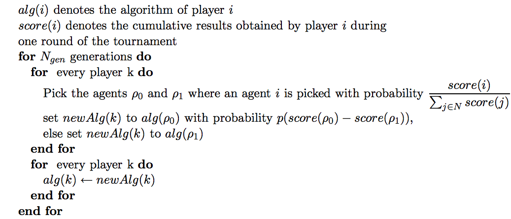
Figure 1. Modified Tournament Selection Algorithm for a population of N agents

2.8
The tournament selection mechanism presented in (Deb 1991) selects the best of the two algorithms with a fixed probability p with 0.5 < p ≤ 1 . In order to facilitate convergence to an equilibrium distribution, we replace this fixed probability by an increasing function p of the score difference. When the score difference is large, the best of the two algorithms is selected with a high probability. This models the situation that a player will be able to differentiate more readily between two players if the score difference is large. If the score difference is small, however, this difference may not be convincing enough to prefer one algorithm over the other. Accordingly, when the score difference is small, we select the best algorithm with a probability close to 0.5. For intermediate score difference, an interpolated probability for selecting the better performing algorithm can be used (see below for more detail).

* Game-playing Algorithms

3.1
We chose well-known learning and non-learning algorithms for the agent populations in our tournaments. We also include one algorithm that was the winner in a local competition among university students. The algorithms used in our tournaments are:

3.2
We believe that not all of these algorithms would be used equally often in an open environment. It seems reasonable to assume that simple algorithms such as R, GTFT, BR and M would be commonly used. In addition, Nash, because of the popularity of the concept of the Nash equilibrium, and FP, as the basic learning approach, are also likely to be used. Under the assumption that a large proportion of agents are learning, a minority of agents can possibly consider using Bully. We consider Saby as an algorithm that may be used by a very small minority of players, since it is not a well-known algorithm. We have not considered pure strategy players, i.e., players who always choose a specific action, as the semantics of any action varies considerably over the different games.

3.3
In our study, we are interested in two properties for characterizing the game-playing algorithms: the sophistication of the algorithm and whether learning is used.

Simple versus Sophisticated algorithms

3.4
Random (R), Generalized-Tit-For-Tat (GTFT), Best Response (BR) and MaxiMin (M) are considered to be simple algorithms. The random algorithm can be interpreted as the ensemble of behavior of a collection of different unidentified algorithms as well as behavior exhibited by inconsistent players. On the other hand, we hypothesize that playing Nash equilibrium (N) is a sophisticated algorithm since there is no known algorithm that computes a Nash equilibrium for an arbitrary game in polynomial-time (Conitzer & Sandholm 2003). In addition, fictitious play (FP), Best Response to FP, Bully and Saby are considered to be sophisticated algorithms as familiarity with the game theory literature is probably necessary for someone to develop or encode them.

Learning versus Non-learning algorithms

3.5
Random, Nash, MaxiMin, and Bully are static algorithms that do not respond to the opponent. GTFT and BR are simple, purely reactive algorithms that can be considered as primitive learning algorithms. An agent using GTFT mimics the last action of the opponent. Instead of mimicking the last action, an agent using BR plays the best response to that action. The remaining algorithms are learning algorithms. The FP algorithm is the basic learning approach widely studied in the game theory literature. If we assume that many agents are using this basic learning approach, it can be beneficial to use an algorithm which plays optimally against FP. Hence we use BRFP. The Saby algorithm presented above is also a learning approach that assumes its opponent to consistently respond to its move in the immediately previous iteration.

* Experimental results

4.1
In the following, we first present results from a round-robin competition with one player per algorithm. This provides a ranking between all the algorithms and head-to-head results that can be used to simulate runs of the evolutionary tournament. Then, we present results from the evolutionary tournament with different selection mechanisms.

Round-robin competition with one player per algorithm

4.2
In this section, our goal is to evaluate relative performances of representative learning and non-learning approaches on a neutral but extensive testbed against a collection of opponents. In the tournament we ran, each algorithm introduced in the previous section is represented by one player. The maximum (minimum) possible payoff to an agent in any iteration is 4 (1). Each player plays every other player including itself, both as row and column player for n iterations of each of the 57 games of the testbed. We first ran experiments to determine the number of iterations to be used for the tournament. For a given number of iterations, we ran 20 tournaments, and the corresponding scores are presented in Figure 2. The ranking of FP and Saby oscillates early on. With more iterations (more than 200), FP ranks first. This result suggests that the learning strategies are performing well, even with a small number of itereations. More iterations enable the learning strategies to be better tuned. Also, since the score is the total number of points accumulated over all the games played, increasing the number of iterations minimizes the impact of the initial period of exploration for the learners. Large number of iterations gives an advantage to learning strategies over fixed strategies. We can also note that BRFP and BR reach the same performance level after 500 iterations. The rankings of Nash and Bully remains the same thereafter.

Figure Figure
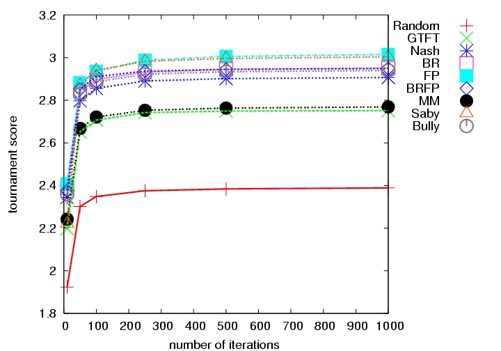
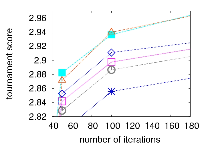
Zoom around iteration 100
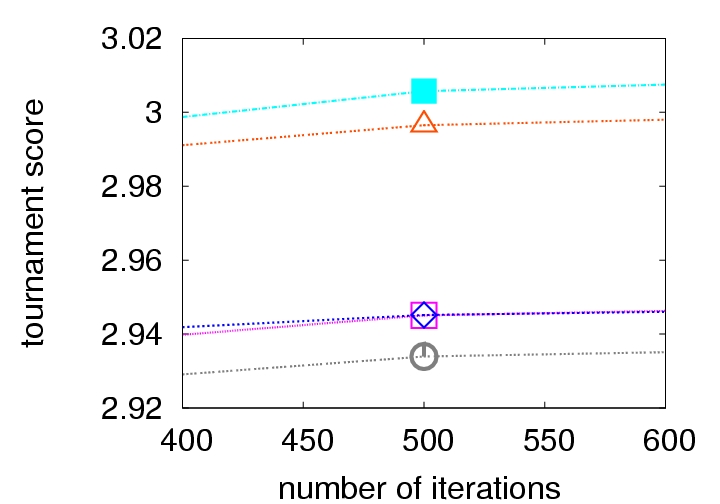
Figure
All iterations Zoom around iteration 500
Figure 2. Choice of the number of iterations

4.3
For all the following experiments, we use the results of the tournament with 1000 iterations. Table 1 contains the average score and standard deviation over all the games of the testbed for one round-robin competition. The player using fictitious play wins the tournament, followed closely by a player using Saby. Note that BRFP, FP and Saby, which are learning approaches that model their opponent's behavior, take three of the first four places. It was surprising to see that best response to last move (BR), a simple, reactive algorithm, outperforms the Nash player. Also, there is no statistical difference between BR and BRFP. The Nash player, which models its opponent as a rational player, comes in at the sixth position. The generalized tit-for-tat player (GTFT), a good choice in a tournament setting involving only the Prisoners' Dilemma game, turns in a relatively disappointing performance and finishes ahead of only the random player.

Table 1: Algorithm ranking based on round-robin competition with one player per algorithm

Rank Avg Score Algorithm std
1 FP 3.014 0.002
2 Saby 3.003 0.004
3 BR 2.951 0.003
BRFP 2.949 0.000
5 Bully 2.939 0.000
6 Nash 2.906 0.000
7 M 2.768 0.000
8 GTFT 2.751 0.008
9 R 2.388 0.001

4.4
Two observations are noteworthy in these results. First, the three learning players perform better than the Nash player. It might be the case that the other players are taking advantage of the randomness introduced in the Nash player (in the cases where there are multiple Nash equilibria, or in the case when the Nash equilibrium is a mixed strategy) [3]. It can also be the case that learning players play better against sub-rational algorithms like BR. The second point of interest was the high ranking of BRFP: one can expect that the performance of the best response to fictitious play will outperform FP. However, it was not clear how well BRFP would do against other players. One possible explanation is that perhaps BRFP is exploiting FP to obtain a large payoff, and performing only satisfactorily against other players. To understand better this overall result, we analyze the head-to-head performance of the algorithms in the round-robin competition, presented in Table 2.

Table 2: Head to head results - mean of the score over all interactions, obtained by the row player in the table, while playing against the column player in the table.

Rank Avg Score Algorithm FP SabyBRBRFPBullyNashMGTFTR
1 3.014 FP 2.950 2.950 3.027 2.999 3.081 2.943 3.081 3.101 2.994
2 3.003 Saby 3.090 2.986 3.040 2.934 3.080 2.929 3.079 2.989 2.904
3 2.951 BR 3.016 2.995 2.901 2.919 3.081 2.931 3.081 2.720 2.910
4 2.949 BRFP 3.040 3.122 3.133 2.906 2.797 2.921 2.884 2.858 2.879
5 2.939 Bully 3.116 3.116 3.116 2.871 2.696 2.891 2.783 2.976 2.888
6 2.906 Nash 2.908 2.930 2.926 2.930 2.811 2.933 2.898 2.922 2.899
7 2.768 M 2.696 2.698 2.696 2.713 2.626 2.734 2.626 3.134 2.994
8 2.751 GTFT 2.728 2.921 2.830 2.880 2.880 2.932 2.582 2.510 2.495
9 2.388 R 2.375 2.391 2.402 2.355 2.311 2.363 2.310 2.494 2.494


Table 3: Head-to-head performance - net score difference of the row player in the table when playing against the column player in the table

Algorithm FP SabyBRBRFPBullyNashMGTFTR
FP   -0.140 0.011 -0.040 -0.035 0.035 0.385 0.373 0.618
Saby 0.140   0.044 -0.188 -0.035 -0.001 0.380 0.067 0.513
BR -0.011 -0.044   -0.214 -0.035 0.004 0.385 -0.110 0.508
BRFP 0.040 0.188 0.214   -0.074 -0.009 0.170 -0.021 0.524
Bully 0.035 0.035 0.035 0.074   0.080 0.157 0.096 0.577
Nash -0.035 0.001 -0.004 0.009 -0.080   0.163 -0.010 0.535
M -0.385 -0.380 -0.385 -0.170 -0.157 -0.163   0.551 0.683
GTFT -0.373 -0.067 0.110 0.021 -0.096 0.010 -0.551   0.000
R -0.618 -0.513 -0.508 -0.524 -0.577 -0.535 -0.683 -0.000  


Table 4: Head to head results - standard deviation of the score obtained by the row player in the table while playing against the column player in the table (the value of the standard deviation is the value of an entry times 10-3)

Algorithm FP SabyBRBRFPBullyNashMGTFTR
FP 0.00 0.21 0.00 0.00 0.00 0.50 0.00 6.34 0.42
Saby 0.20 2.69 3.04 0.18 0.00 0.36 0.02 0.29 0.59
BR 0.00 3.15 0.00 0.00 0.00 0.41 0.00 9.69 0.49
BRFP 0.00 0.22 0.00 0.00 0.00 0.34 0.00 0.00 0.39
Bully 0.00 0.00 0.00 0.00 0.00 0.36 0.00 0.00 0.47
Nash 1.55 0.40 0.39 0.29 0.24 0.34 0.21 0.53 0.53
M 0.00 0.02 0.00 0.00 0.00 0.50 0.00 0.00 0.73
GTFT 9.28 8.03 6.36 0.00 0.00 0.35 0.00 0.56 0.53
R 1.92 0.62 0.49 0.45 0.52 0.77 0.45 0.51 0.50

4.5
We now describe head-to-head results over the 57 games, presented in Table 2. This table contains the average score obtained by the algorithm whose name is on a row while playing against the algorithm whose name is on a column averaged over 20 instances of the tournament. We can then compute the net difference of scores of the players by subtracting from Table 2 its transpose, and these results are presented in Table 3. When an entry of Table 3 is positive, the row player is winning against the column player, whereas the opposite is true when the entry is negative. The head-to-head results have a small standard deviation (see Table 4) due to the use of learning and random players. These head-to-head results lead to the following conclusions:

Evolutionary Tournament

4.6
In this section, we investigate the effect of an evolutionary mechanism upon the algorithm distribution in a finite-size population playing a round-robin competition at each generation. We want to find out the existence and the nature of the equilibrium algorithm distribution of the population and the rate of convergence to that distribution when agents adopted relatively successful algorithms in the previous generation. These simulations correspond to real life marketplace dynamics where agents adopt relatively successful decision mechanisms in their environments. We investigate a sequence of scenarios where we incrementally introduce more sophisticated algorithms in the initial population.

4.7
We run tournaments with a population of 10,000 agents where the algorithms may or may not be uniformly distributed (all algorithms have equal representation). To save computational cost, we simulate the tournament to avoid running the actual round-robin competition at each generation. For a game between two players p1 and p2, the score obtained by pi, i ∈{1,2}, is a sample drawn from a normal distribution of the corresponding mean and variance from Table 2 and Table 4 respectively. This approximates the actual tournament since we draw the scores from independent distributions.

4.8
For the function p , the probability to pick the best of the two algorithms, in Figure 1, we chose a linear function of the score difference. Table 3 provides the score difference between the algorithms. We picked a value δmax that is larger than any score difference, and we used the function p(δ)=½(1+δ/δmax). When δ is close to zero, p is close to ½ and when the score difference is larger, tends to 1. In the experiments presented in this paper, we use δ=0.7.

Experimental results from evolutionary tournaments

4.9
We now present results from evolutionary tournaments with different initial population compositions. We start by showing results of a population that uses only simple algorithms. We then present experiments where more sophisticated algorithms are present in the initial population. We show that a small number of agents using sophisticated algorithms can substantially alter the dynamics of the evolution of the population. These experiments are performed using the traditional and modified tournament selection mechanisms. The last set of experiments compares the populartion dynamics when the three different selection mechanisms are used.
Simple Algorithms and injection of few rational players

4.10
In the first set of experiments, we consider a population of agents using simple algorithms: the initial population is composed of agents using R, GTFT, M, and BR, with 2,500 agents representing each algorithm. This population quickly converges to a population using exclusively BR. To observe the effects of a more complex algorithm in a mixed of these simple algorithms, we introduce a small number of agents using Nash (N): 1% of the agents initially uses N, the rest of the population uses the other algorithms in equal proportions. We observe that even with such small initial proportion of agents using N, N takes over the entire population. The corresponding population dynamics is represented in Figure 3. We show the results with two selection mechanisms: tournament selection and its modification. We can see that convergence is faster with the modified tournament selection. This conclusion will also be corroborated in other experiments later in the paper.

4.11
From the head-to-head results of Table 2, we can infer that the performance of BR and Nash should be similar in this population. The payoffs obtained by these two algorithms against the other algorithms are very close except against M and GTFT: compared to N, BR gets a higher payoff against M, but N does better against GTFT compared to BR. From Table 2 again, we can see that BR should perform better than M (M is better than BR against GTFT and R, but BR is better in self-play and against N, M and GTFT), which explains why the percentage of agents using BR grows faster than the percentage of agents using M in the first iteration. R, GTFT and M, which perform worse than N and BR, become extinct. When only BR and N remain, BR is slightly better than N in head-to-head matches, but the difference is negligible compared to the self-play performance where N does slightly better. Hence, the population converges to N.

4.12
These results show that the Nash algorithm dominates the population when pitted against static or simple reactive algorithms and this result is primarily due to better self play. This is akin to the tit-for-tat strategy's success in PD tournaments involving heterogeneous strategies.

Figure Figure
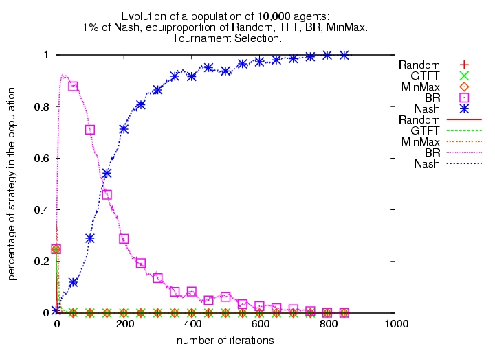
Figure 3. Evolutionary Tournament with 5 algorithms (1% Nash and equal proportion of R, GTFT, BR and M) with tournament selection (left) and modified tournament selection (right)

Introducing FP

4.13
In the next set of experiments (see Figure 4), the initial population contains 1% of learning agents using the FP algorithm, and the remaining population uses R, GTFT, N, BR and M in an equal share. This configuration gives rise to an interesting dynamics: 1) the Nash algorithm is initially adopted by a significant portion of the population, but thereafter decreases in popularity and becomes rapidly extinct; 2) the population of agents using BR first increases and then stabilizes at a slightly lower value; 3) the learning algorithm FP, even when initially used by a minority of the population, is ultimately preferred by a majority of the population members and reaches a mixed equilibrium with BR.

4.14
During the first few generations, agents using FP obtain the best score. From Table 2 and 3, we see that FP scores more than N against all opponents. In addition, FP scores more than BR against BR, N, GTFT and R. Also, FP and BR perform equally well when they play against M, but BR scores more than FP when playing against FP. This explains that, during early generations, FP scores better, hence more agents adopt this algorithm. Among the remaining algorithms, as noticed above, agents using BR and N perform the best, with a marginal advantage for N, and the other algorithms are exploited. During the first few iterations, since the number of agents using FP is small, the behavior of the Nash and BR algorithm resembles the dynamics in Figure 3: the Nash algorithm is preferred by most of the population. When R, GTFT and M become extinct, some agents in the population are still using the BR algorithm. Thereafter, when only BR, N and FP are present, the population converges to a mixed population of agents using FP and BR. We can see in Table 3 that N loses head-to-head competing against BR and FP. Although Nash performs better than BR in self-play, it is not enough to counter the head-to-head losses and hence the agents abandon the Nash algorithm. Note that BR loses head-to-head against FP (by a small margin) and that FP performs better in self-play. Hence when an equal number of agents use each algorithm, more agents will adopt FP. From Table 2, we see that when the opponent is an FP player, an agent using BR scores more than an agent using FP, and the results are reversed when the opponent is a BR player. These performance differences allow for a mixed equilibrium, when 65.6% of the population uses FP[4], as observed in Figure 4. We do observe minor fluctuations around the theoretical fixed point due to sampling error from a finite population. The convergence to a stable population with different strategies is an interesting example of mutual dependence of these strategies.

There are two important observations from this representative population:

Figure Figure
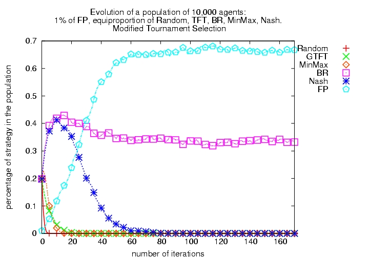
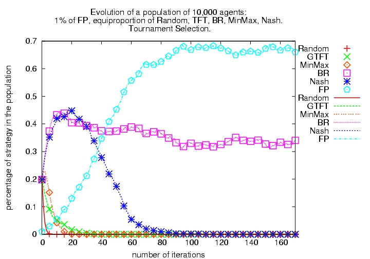
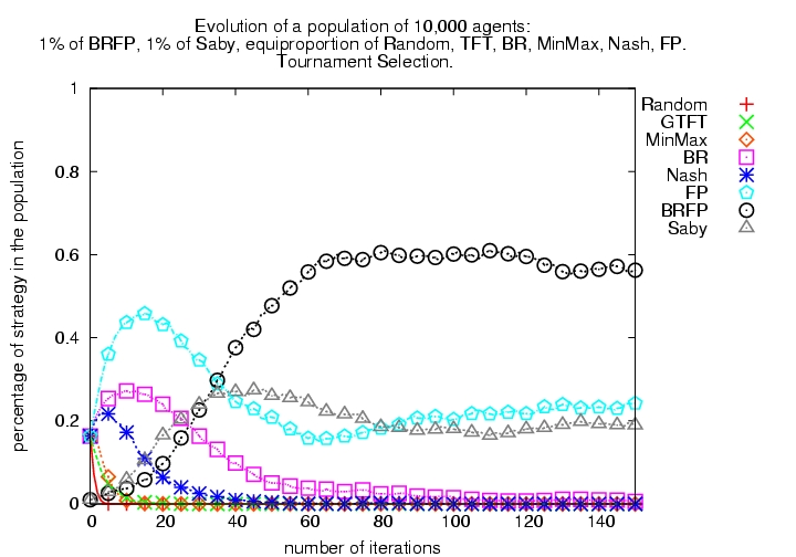
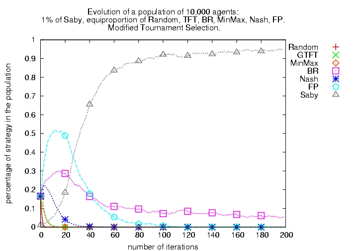
Figure 4. Evolutionary Tournament with 6 algorithms (1% FP and equiproportion of R, GTFT, BR, MaxMin, Nash each) with tournament selection (left) and modified tournament selection (right)

Introducing BRFP and Saby

4.15
Next, we ran an experiment where Saby and BRFP are used by 1% of the population each and R, GTFT, BR, M, Nash and FP are used in equal proportion by the remaining population. The outcome of the evolutionary tournament (see Figure 5) is a mixed population of agents using Saby, FP, and BRFP. We conclude that more sophisticated learning players will eventually dominate the population if agents adopt algorithms that are more successful. The theoretical equilibrium occurs for 21.8% of agents using FP, 58.1% of agents using BRFP, and 20.1% of agents using Saby. Given the results of the round-robin competition (4.2), it is not as a surprise that these three algorithms do well. It is interesting, however, to observe a mixed equilibrium distribution. It is also interesting that the algorithm that wins the round robin competition (4.2) does not have the larger share of the population. This is due to the fact that, if the competition was limited to only these three strategies, BRFP would place first, followed by FP and then Saby. From Tables 2 and 3 we can see that BRFP wins head-to-head against both FP and Saby, and it is therefore not surprising that BRFP is used by the majority of agents. It is interesting to note, however, that although FP loses head-to-head against both Saby, and BRFP, it still survives the evolutionary process. When we examine the scores obtained by FP, Saby and BRFP against BRFP in Table 2, we see that FP's results are higher than Saby and BRFP. Hence, if the proportion of BRFP is large, FP agents will be able to gain from their presence. Saby agents are losing head-to-head against BRFP agents, but they can make up by exploiting FP agents.

Figure Figure
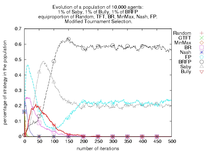
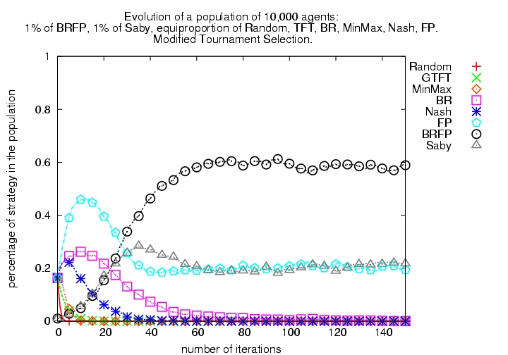
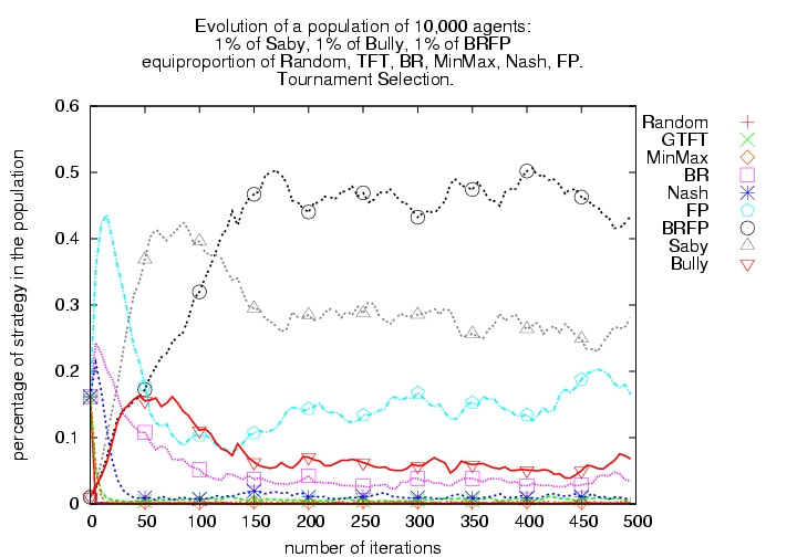
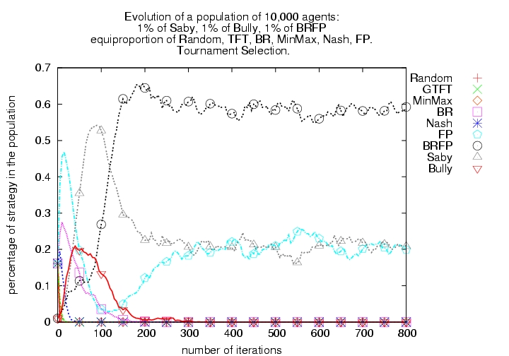
Figure 5. Evolutionary Tournament with 8 algorithms (1000 each of R, GTFT, BR, M, Nash, FP, BRFP, Saby), using modified tournament selection

Experiments with Bully

4.16
BRFP agents assume that a significant proportion of agents in the population use FP and plays optimally against these agents. If a significant proportion of agents are using learning algorithms, one can use the static Bully algorithm that leads the learner to play an action that is beneficial to Bully. In the next set of experiments, we first consider an initial population containing the simple algorithms with FP and Saby, but no agent using BRFP. This population converges to a mixed population where agents using Saby and BR algorithms coexist (see Figure 6). We next introduce a few agents using Bully. Interestingly, the corresponding graph from Figure 6 shows that even when a small initial proportion of agents use Bully, they are able to survive by exploiting agents using Saby. In both of these situations, agents using FP are exploited mainly by agents using Saby, and FP becomes extinct after a few iterations. In the presence of the Bully algorithm, the population converges to a distribution where Saby, BR and Bully coexist. Even though Bully is not able to dominate the population, its presence has a tangible impact on the evolutionary dynamics. It is also interesting to note, as shown in Table 3, that Bully does not lose head-to-head against any other algorithm. It, however, does not perform well in self play. These experiments show that stationary algorithms can survive by exploiting learning ones.
Tournament Selection Modified Tournament Selection
No Bully initially present Figure Figure
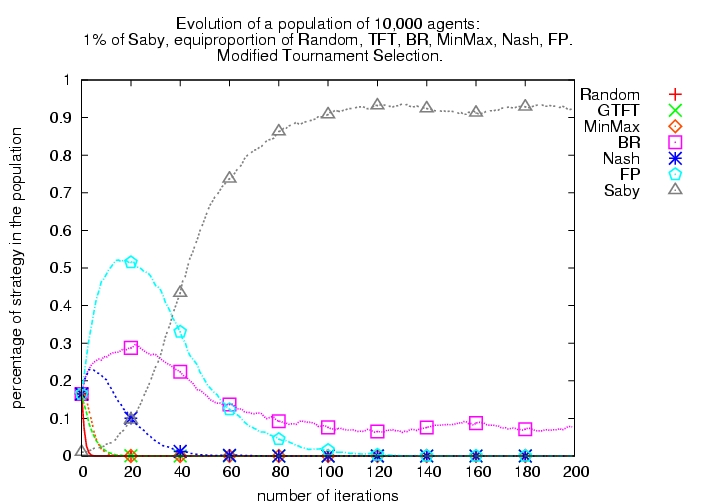
Small proportion of Bully initially present Figure Figure

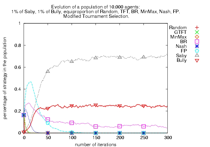
Figure 6: Evolutionary tournaments including learning algorithms with or without Bully

Comparison of different selection mechanisms when all the algorithms are present.

4.17
In the previous experiments (Figure 3, 4, 5 and 6), we provided results from the Tournament selection and its modification. These figures show that the modified tournament selection scheme converges faster in general than the traditional tournament selection and that both schemes produce the same equilibrium. In this section, we describe results from simulations where all algorithms listed in section 3 are present in the initial population and we study the dynamics of the population with three different selection mechanisms. We assume that a relatively small proportion of agents (1%) use the complex algorithms Bully, BRFP, and Saby in the initial population while the rest of the population is equally distributed among the simple algorithms. Results from experiments with different selection mechanisms are presented in Figures 7a, 8a and 9. All the three selection mechanisms converge to a mixed population of agents using Saby, FP and BRFP algorithms. It is also interesting to note that the three selection mechanisms have similar dynamics, albeit on different scales. At the beginning, as expected from the head-to-head results presented in Table 2, Nash, BR, FP, Saby, BRFP and Bully increase in proportion in the population. Random, MinMax and GTFT decrease and disappear from the population. Then, as observed in previous cases, the percentage of agents using Nash decreases, due to its exploitation by the learning strategies. The next "victim" of the presence of the learner and Bully is BR. Subsequently, because of the presence of more agents using FP, BRFP agents profit from the increased exploitation opportunity. Hence, the proportion of FP agents decreases and the proportion of BRFP agents increases. Then, the proportion of Bully, which was growing at the same speed as the proportion of Saby, starts to decrease due to its relatively low score on self play and because there are less BR and FP agents that Bully can exploit. When the proportion of Bully agents starts to decrease, the proportion of BRFP increases at a faster rate. Bully is the only algorithm that defeats BRFP in the current population. As BRFP increases, Saby starts to decrease (from Table 2 and 3, BRFP defeats Saby). Finally, with lower percentage of Saby, FP makes a comeback and the population reaches a mixed equilibrium with a large fraction of BRFP agents and a smaller, roughly equal, share of Saby and FP agents. This equilibrium is the same as above.

Figure Figure
(a) Modified tournament selection (b) 99% Modified tournament selection and 1% random selection

Figure 7: Modified tournament selection with all algorithms.

Figure Figure
(a) Tournament selection (b) 99% Tournament selection and 1% random selection

Figure 8: Tournament selection with all algorithms.

4.18
Tournament selection needs 300 iterations to converge when the modified tournament selection needs 200 iterations to reach equilibrium (see Figure 7a and Figure 8a respectively). As expected, the modification of the selection scheme with stronger selection bias leads to faster convergence. Experiment using the fitness proportionate selection mechanism (see Figure 9) produces near-equilibrium distributions after more than 1,200 iterations. This is much slower compared to the other selection mechanisms. The equilibrium reached by the fitness proportionate selection mechanism is 'smoother' than the equilibrium obtained by the tournament selections: tournament selection and its variant result in populations oscillating around the theoretical equilibrium distribution, which is due to higher sampling noise in those schemes.

Figure
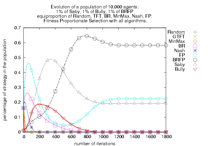
Figure 9. Fitness Proportionate Selection with all algorithms

4.3.6 Noisy Selection

4.19
We also performed experiments where agents select a strategy at random with a probability of 0.01 for the tournament-based selection mechanisms. This corresponds to random error or noise in the selection procedure and can ensure preservation of all algorithms in the population. Hence, the nature of the equilibrium is slightly different. Addition of random selection does not significantly alter the speed or nature of convergence (see Figures 7b and 8b), although we observe small oscillations around the equilibrium in both tournament selection and its modification. We believe that the random selection of the two agents in the tournament selection incorporates some noise in the selection process and hence, the effect of minor additional noise has no substantial effect. The additional random selection, however, ensures that all algorithms are present in the final population, albeit in very small proportion. The primary beneficiary of this process is the Bully algorithm as it has the highest surviving percentage among algorithm s that did not survive without this selection noise. Compared to experiments without random selection where Saby and FP have almost an equal share at equilibrium, the introduction of noise increases Saby's share and decreases FP's share.

* Conclusion

5.1
We have evaluated several representative learning and non-learning algorithms using an evolutionary tournament where agents adopt relatively successful algorithms from the previous generation. During each generation, a round-robin competition is played over a testbed of two-player two-action iterative single stage games. The testbed consists of all structurally distinct 2×2 conflicted ordinal-preference games and provides a fair and extensive set of testing scenarios. Evolutionary tournaments provide valuable insights into the performance of decision mechanism in real-life marketplaces where users are likely to adopt those strategies that have been observed to return higher payoff in their environment. Correspondingly, these results also allow us to choose decision strategies to use in such dynamic market conditions. Hence, experiments like ours are likely to be of more benefit compared to work on static analysis of equilibrium strategies for choosing decision procedures for open, adapting marketplaces consisting of a diversity of competitors with varying expertise, knowledge and capabilities.

5.2
When we consider only a round-robin competition with one player per algorithm, the Nash player is dominated by learning approaches. Though the actual ranking is dependent on the exact set of players involved, it can be argued that the learning players will typically outperform non-learning players when there is a variety of players in the tournament. We also notice that the learning players perform better in self-play. This is because most static strategies and even Nash equilibrium are not necessarily efficient, i.e. they may not produce Pareto-optimal outcomes. It also came as a surprise that, averaged over all the games in the testbed, the Nash player could significantly outperform only the random player. In addition, the fictitious play player loses out to the player who plays best response to it, and can only fare well by outperforming the random player.

5.3
In the evolutionary tournament, the learning algorithms, including fictitious play and a best response to it, outperform players like Nash and survive the evolutionary process: the Nash algorithm cannot survive when learning algorithms are present in the initial population. Learning algorithms may not always take over the entire population and some stationary algorithms, like Bully can coexist with them. To test the robustness of these results, we ran experiments using three different selection mechanisms: fitness proportionate, tournament selection, and a hybrid algorithm designed to increase the speed of convergence that adds a flavor of fitness proportionate in tournament selection. Although the speed of convergence differs, the modified tournament selection being the fastest, the nature of the equilibrium reached with the three selection schemes is similar.

5.4
The performance of the algorithms in this study is aggregated over many games. It would be interesting to provide an analysis tailored for individual or a given subset of games. Also, while the current sets of experiments are run over all structurally distinct conflicted 2×2 games with ordinal payoff, it would be interesting to see if these results generalize to large samples of randomly generated n×n games with cardinal payoff. In this paper, we studied the evolution of population using different initial algorithm distributions. In some cases few good agents can take over an entire population. We are planning to further investigate the effect of initial algorithm distributions on equilibrium distributions and the importance of the selection mechanism used in the evolutionary process. Running similar tournaments with more sophisticated learning algorithms developed recently (Bowling 2005; Barnerjee & Sen 2007; Crandall & Goodrich 2005) can also produce useful insights for their effectiveness in open environments.

* Acknowledgements

This work has been supported in part by an NSF award IIS-0209208.

* Notes

1 A conflicted game is a game where no joint action can provide the most preferred outcome to all players.

2 For a given game in the testbed, there exists structurally equivalent games (that can be obtained by renaming the actions or the players), but none of the equivalent games is present in the testbed. All the games in the testbed are therefore structurally distinct. For each game structure, our selection of the representing matrices has introduced a bias: playing as a column player introduces an advantage.

3 Games with multiple Nash equilibria, rational agents will face a problem of equilibrium selection. Since the agents do not communicate, they may often select different equilibria and hence reach an undesirable outcome. A simple example is the coordination game, where each of the two agents gets 1 if they play the same action and 0 otherwise. There are three Nash equilibria, two pure strategies and one mixed strategy. One pure strategy equilibrium is when both players play the first action and other pure strategy equilibrium is when both players play the second action. In the mixed equilibrium, both the players play each action with probability 0.5. Therefore there is a significant chance that both players end up playing different actions and get 0.

4When there are two algorithms i and j present in the population, we can easily compute the score obtained by any agent as a function of the proportion fi of algorithm i in the population (1-fi is the proportion of algorithm j in the population). From Table 2, let hij denote the score obtained by an agent using algorithm i when playing against an agent using algorithm j. The score of an agent using algorithm i is si(fi)=fi·hii+(1-fi)·hij and the score for agent using algorithm j is sj(fi) = fi·hji+(1-fi)·hjj. If si(fi)>sj(fi) or si(fi)<sj(fi) for all fi∈[0,1], one algorithm will be ultimately used by all agents in the population. Otherwise, there exists a fixed point fi* where the two algorithms coexist: ∃fi*∈[0,1] | si(fi*)=sj(fi*): all the agents have the same score. Let us consider the case where si(fi) is a decreasing function of fi (sj(fi)=1-si(fi) is then an increasing function) and we have ∀fi < fi*, si(fi)>sj(fi) and ∀fi > fi*, si(fi)<sj(fi). For fi < fi*, the number of agents using algorithm i increases since those agents have better performance. However, with the increase in the number of agents using i, the performance of agents using i decreases whereas the performance of agents using algorithm j increases. When fi >fi*, agents using the algorithm j outperform those using algorithm i and hence, the proportion of algorithm j now increases. This process repeats until the population reaches the equilibrium point. This shows that the fixed point is an attractor. Similarly, a theoretical equilibrium can be calculated for n strategies by solving the following problem: ∀ (i,j) ri = rj where rij fj hij, Σifi=1 and fi ∈ [0,1] ∀i.


* References

AXELROD R (1985) The Evolution of Cooperation, Basic Books, New York.

AXELROD R (1987) The Evolution of Strategies in the Iterated Prisoner's Dilemma. In Genetic Algorithms and Simulated Annealing, Lawrence Davis (ed.) (London: Pitman, and Los Altos, CA: Morgan Kaufman, 1987), pp. 32-41. Reprinted as Evolving New Strategies, pp. 10-39. in Axelrod, R. M. (1997).

BANERJEE B, Sen S and Peng J (2001) Fast concurrent reinforcement learners. In Proceedings of the Seventeenth International Joint Conference on Artificial Intelligence, 825–830.

BANERJEE D and Sen S (2007) Reaching pareto-optimality in prisoner's dilemma using conditional joint action learning. In Autonomous Agents and Multi-Agent Systems, Volume 15, number 1, August 2007, 91-108, Springer Netherlands

BOWLING M (2005) Convergence and no-regret in multiagent learning. In Advances in Neural Information Processing Systems 17 , 209-216

BOWLING M and Veloso M (2001) Rational and convergent learning in stochastic games. In Proceedings of the Seventeenth International Joint Conference on Artificial Intelligence, 1021–1026.

BOWLING M and Veloso M (2002) Multiagent learning using a variable learning rate. Artificial Intelligence, 136:215–250.

BRAMS S J (1994) Theory of Moves. Cambridge University Press, Cambridge: UK.

CLAUS C and Boutilier C (1998) The dynamics of reinforcement learning in cooperative multiagent systems. In Proceedings of the Fifteenth National Conference on Artificial Intelligence, 746–752. Menlo Park, CA: AAAI Press/MIT Press.

CONITZER V and Sandholm T (2003) Complexity results about Nash equilibria. In Proceedings of the Eighteenth International Joint Conference on Artificial Intelligence (IJCAI), 2003.

CRANDALL J W and Goodrich M A (2005) Learning to Compete, Compromise, and Cooperate in Repeated General-Sum Games. In Proceedings of the 22nd International Conference on Machine Learning, 161-168.

DEB K and Goldberg D (1991) A comparative analysis of selection schemes used in genetic algorithms. In Rawlins, G. J., ed., Foundations of Genetic Algorithms, 69–93. San Mateo, CA: Morgan Kaufman.

NUDELMAN E, Wortman J, Shoham Y and Leyton-Brown K (2004) Run the GAMUT: A Comprehensive Approach to Evaluating Game-Theoretic Algorithms. In Proceedings of the third International Joint Conference on Autonomous Agents and Multiagent Systems(AAMAS'04).

FUDENBERG D and Levine K (1998) The Theory of Learning in Games. Cambridge, MA: MIT Press.

GREENWALD A and Hall K (2003) Correlated-q learning. In Proceedings of the Twentieth International Conference on Machine Learning, pages 242-249.

HU J and Wellman M P (1998) Multiagent reinforcement learning: Theoretical framework and an algorithm. In Shavlik, J., ed., Proceedings of the Fifteenth International Conference on Machine Learning, 242–250. San Francisco, CA: Morgan Kaufmann.

JAFARI A, Greenwald A, Gondek D and Ercal G (2001) On no-regret learning, fictitious play and Nash equilibrium. In Proceedings of the Eighteenth International Conference on Machine Learning, 226-233, San Francisco, CA: Morgan Kaufmann.

LITTMAN M L and Stone P (2001) Implicit negotiation in repeated games. In Intelligent Agents VIII: AGENT THEORIES, ARCHITECTURE, AND LANGUAGES, 393–404. Littman, M. L. 1994. Markov games as a framework for multi-agent reinforcement learning. In Proceedings of the Eleventh International Conference on Machine Learning, 157–163. San Mateo, CA: Morgan Kaufmann.

LITTMAN M L (1994) Markov games as a framework for multi-agent reinforcement learning. In Proceedings of the Seventh International Conference on Machine Learning, 157-163.

LITTMAN M L (2001) Friend-or-foe q-learning in generalsum games. In Proceedings of the Eighteenth International Conference on Machine Learning, 322–328. San Francisco, CA: Morgan Kaufmann.

MCKELVEY R D, McLennan A M, and Turocy T L (2005) Gambit: Software Tools for Game Theory, Version 0.2005.06.13. http://econweb.tamu.edu/gambit

MUNDHE M and Sen S (2000) Evaluating concurrent reinforcement learners. In Proceedings of Fourth International Conference on MultiAgent Systems, 421–422. Los Alamitos, CA: IEEE Computer Society.

SANDHOLM T and Crites R (1995) Multiagent Reinforcement Learning in the Iterated Prisoner's Dilemma. In Biosystems 37(1:2).

----

ButtonReturn to Contents of this issue

© Copyright Journal of Artificial Societies and Social Simulation, [2007]