Jijun Zhao, Ferenc Szidarovszky and Miklos N. Szilagyi (2007)

Finite Neighborhood Binary Games: a Structural Study

Journal of Artificial Societies and Social Simulation vol. 10, no. 3 3
<https://www.jasss.org/10/3/3.html>

For information about citing this article, click here

Received: 22-Jun-2006    Accepted: 11-Feb-2007    Published: 30-Jun-2007

Abstract

The purpose of this study is to present a systematic analysis of the long-term behavior of the agents of an artificial society under varying payoff functions in finite neighborhood binary games. By assuming the linearity of the payoffs of both cooperating and defecting agents, the type of the game is determined by four fundamental parameters. By fixing the values of three of them and systematically varying the fourth one we can observe a transition from Prisoner's Dilemma to Leader Game through Chicken and Benevolent Chicken Games. By using agent-based simulation we are able to observe the long-term behavior of the artificial society with different and gradually changing payoff structure. The difference between different games is explored and the effect of the transition from one game to the other on the society is investigated. The results depend on the personality types of the agents. In this study greedy and Pavlovian agents are considered. In the first case, we observe the most significant change in trajectory structure between Prisoner's Dilemma and Chicken Games showing significant difference in the behavioral patterns of the agents. Almost no changes can be observed between Benevolent Chicken and Leader Games, and only small change between Chicken and Benevolent Chicken. The trajectories change from always converging to regularly oscillating patterns with systematically altering amplitude and central values. The results are very similar whether the agents consider themselves as members of their neighborhoods or not. With Pavlovian agents no significant difference can be observed between the four games, the trajectories always converge and the limits smoothly and monotonically depend on the value of the varying parameter.

Keywords:

Agent-Based Simulation, N-Person Games, Structure Analysis, Equilibrium

Introduction

1.1

One of the most commonly used methods of investigating multiperson games is agent-based simulation. There is a large literature (see for example Rapoport and Guyer 1966) on the different types of games, the different types of behavior of the players in those games and how this behavior affects the outcomes. The simplest games are those that are symmetric, in which the players (or agents) have only two available choices and only the preference orderings of the payoffs are taken into account. Rapoport and Guyer (1966) have shown that there are 576 different types of such two-person games, or 78 if the players and their payoffs are interchanged. In the case of N-person games, this number is much larger. It is assumed that the payoff for each agent depends on the ratio of agents having a particular choice. If we call the choices cooperation (C) and defection (D) and the number of cooperators among the N agents is k, then the payoff for a cooperating agent is C(k/N) and that for a defecting agent is D(k/N) where C and D are real valued functions in the unit interval [0, 1]. Therefore the outcome and the entire evolution of the game depend on only the relative order of the values C(0),C(1/N), … ,C(N/N),D(0), D(1/N), … ,D(N/N). If no special condition is assumed about functions C and D, then there are (2N+2)! possible orderings of these values, so this is the total number of possible game outcomes and dynamic evolutions. 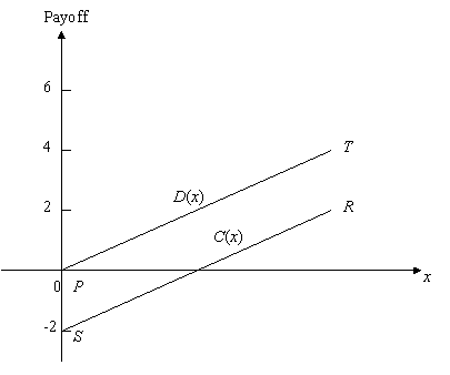If we assume that both functions C and D are strictly monotonic then the orders of subsequences C(0),C(1/N), … ,C(N/N) and D(0), D(1/N), … ,D(N/N) are given, so there are only possibilities for mixing the two sequences. If we assume furthermore that both functions are linear, then this number can be reduced. Merlone et al. (2007) discuss this case and give a tight upper bound for this number. Similar situations occur if the payoffs of each agent depend on the ratio of cooperators in a defined neighborhood about the agent. In this case N has to be replaced by the number of agents located in the neighborhood. If both functions C and D are linear (see Figure 1, where C(x)=(R-S)x+S and D(x)=(T-P)x+P), then the games are well defined by the numbers P=D(0), T=D(1), S=C(0) and R=C(1).

Figure 1. Payoff functions

1.2

There are 4!=24 different orderings of these values which generate 24 different games. The most frequently discussed game is the Prisoners' Dilemma, in which S<P<R<T. A comprehensive summary of N-person Prisoners' Dilemmas is given in Szilagyi (2003) and a special simulation tool designed for unlimited number of agents with user-defined parameters is introduced in Szilagyi and Szilagyi (2000). There is also a large variety of behavior types of the agents. For some particular types see for example, Helbing et al. (2000), Kitts (1999), Panzarasa et al. (2001) and Panzarasa and Jennings (2001). A continuous time scale version of N-person prisoners' dilemma is developed and analyzed in Zhao et al. (2007). Other game types are also frequently discussed in the literature; however there has not been any attempt to the systematic analysis of the different games as parameter values change. This analysis would show how one game evolves into another game, how the outcomes and dynamic evolution of the games depend on the changing parameter values and what happens at and around the boundary between two games. This structural analysis can serve several purposes. It presents a systematic analysis of the transition between certain pairs of games, shows the properties of the game at and around the border line between games, and helps to design special parameter values to ensure desired behavioral patterns of the agents. Moreover, the examination of the boundary region between two games provides similar information than those obtained in the bifurcation theory of dynamic systems, which have significant theoretical interest.

1.3

In this paper we will present the first attempt of such structural analysis. We selected four games, the Prisoners' Dilemma, Chicken, Benevolent Chicken and Leader Games from the large set of binary games. The reason for this choice is as follows. Szilagyi (2005) claims that a game can be considered a dilemma only if reward for mutual cooperation is greater than the punishment for mutual defection, but the temptation to defect, that is, defecting alone, gives the largest possible outcome. Mathematically these conditions can be given as P<R<T. Fixing the values of P, R and T and gradually changing the value of S we have 4 possibilities (excluding the border-line cases). If S<P, then the game is the well-known Prisoners' Dilemma (Szilagyi 2003), if P<S<R, then it is the Chicken Game (Szilagyi 2007). The case of R<S<T gives the Benevolent Chicken Game (Zizzo 2006) and if S>T, then we have the Leader Game (Guyer and Rapoport 1969). By using agent-based simulation we will give a systematic description of the transformation of the game from Prisoners' Dilemma to the Leader Game and present the characteristics of changing from one game to another. Other cases can be examined in a similar way and they will be the subjects of our future works. In this study we will concentrate mainly on the effect of neighborhood structure, different updating strategy is also an interesting topic. For particular game classes it has been already examined and known from the literature (see for example,Szilagyi 2003). The simulation process and the computational results will be presented in the next two sections and final conclusions will be outlined in Section 4.

Simulation Methodology

2.1

We assume that the agents are distributed on and fully occupy a finite two-dimensional space. In this study we select the integer points (i, j) with 1≤ i ≤100 and 1≤ j ≤100. Therefore the number of agents is N=10,000. The neighborhood of each agent is given by one layer, so that an agent (k, l) belongs to the neighborhood U(i, j) of agent (i, j), if and only if |k-i|≤1 and |l-j|≤1. Notice that U(i, j) has 9 neighbors (including agent (i, j)) unless agent (i, j) is on the boundary. In this case U(i, j) has 4 or 6 neighbors depending on whether agent (i, j) is located on a corner or not. We fix the values of P=D(0)=0, R=C(1)=2 and T=D(1)=4 and systematically vary the value of S=C(0) from -2 to 6. Only linear functions C and D are considered. Let x denote the ratio of cooperators in the neighborhood of agent (i, j), then its payoff is C(x) if it is a cooperator, and D(x) if a defector. As it was mentioned earlier, there are many possible behavior types of the agents. In our study we assume a special adjustment process. At each time period t=0,1,2,…,T, the state of the system consists of the choices (C or D) of the agents. Therefore there are 2^N possible states of the system. The dynamic process starts at a given initial state and its evolution depends on the personality of the agents. In this paper, we will consider two types of personalities: greedy and Pavlovian. A greedy agent always imitates the action of its neighbor with the highest reward. For a Pavlovian agent, if its action is followed by a satisfactory state of affairs, then its tendency to produce that particular action is reinforced. It is assumed first that all agents are greedy (Szilagyi and Szilagyi 2000). At each time period t≥1, each agent (i, j) looks at the payoffs of all agents in its neighborhood (including its own) and selects all those agents who received the highest payoff in the previous time period. If the agent (i, j) is among them, then it keeps the same choice as before. Otherwise it checks the previous choices of the best-awarded neighbors. If all of them had different choice than agent (i, j), then this agent changes its choice to the best-awarded one, otherwise it keeps the same choice what was its selection in the previous time period. Based on this rule, all agents select new choices (by keeping or changing the previous choice) for the new time period. This step is repeated for t=1,2,…,T, so complete choice-trajectories are obtained for all agents and the ratio of cooperators x(t) can be computed at each time period t. Our main concerns are the properties and possible convergence of sequence x(t). In the simulation study to be described in the next section we will illustrate how these properties change if we gradually alter the value of S=C(0) and show how transitions occur between different games. We will later briefly discuss the case of Pavlovian agents.

Simulation Results and Analysis

3.1

As mentioned earlier, we select linear functions for C and D with the fixed values of P=D(0)=0, R=C(1)=2 and T=D(1)=4 and vary the value of S=C(0) from -2 to 6 with a small step size 0.01. The initial state is defined by the initial ratio of cooperators x(0). The cooperating agents are uniformly distributed in the given 100×100 grid according to the initial ratio. Figure 2 shows the final ratios x(100) for the varying values of S and x(0). The patterns of the final ratios as functions of S are very similar for different values of x(0).

3.2

If S<0, the game is the Prisoners' Dilemma, the trajectories x(t) converge immediately or after a few iterations and the limit depends on the initial ratio of cooperators x(0). The effect of S on converging limit is trivial. This is the case even at the boundary with the Chicken game (S=0). The trajectories always converge to 0 when x(0) varies from 0 to a certain value below 0.7, however the limit slightly increases if x(0) becomes larger; for example, it increases from 0.01 (or from 0.0016 depending on S) with x(0)=0.7017 to about 0.051 with x(0)=0.8991. Hence, in a society of only greedy agents with one layer neighborhood, if the environment is for Prisoners' Dilemma, then initial majority of defectors will lead the entire society to defection, while initial majority of cooperators might stabilize the society with a small number of cooperators.

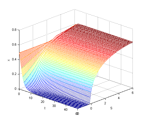
Figure 2. x(100) as a function of S with varying value of x(0)

3.3

For S>0 there is a gap: within the gap, the trajectory x(t) still behaves as Prisoners' Dilemma; after the gap, there is a sudden change in the behavior of the trajectory. If x(0)=0.1, then the trajectory behaves as in the case of Prisoners' Dilemma even for 0<S≤0.25, afterwards the trajectories start oscillating as they should in Chicken Games. The gap keeps the same while x(0) increases until x(0)=0.13. From x(0)=0.13 to x(0)=0.9, the gap is 0<S<0.01. After the gap the trajectories follow the pattern of Chicken Games with oscillations. Figure 3 shows different oscillatory patterns with S=0.01, 1.0 and 1.99 by selecting the initial value x(0)=0.9, and the comparison of these three trajectories indicate that the frequency increases with larger value of S. Table 1 shows the averages of the x(t) values of the last 20 iterations for different values of S and x(0). The elements of the right most column are the calculated standard deviations of the specific rows (averaged x(t) when S is fixed). The elements of the last row are the calculated standard deviations of the specific columns (averaged x(t) when x(0) is fixed). By comparing these two types of standard deviations, it can be observed that the effect of the initial ratio of cooperators to the final result is much smaller than that of the value of S. It is also interesting to notice from the Table that when S is very close to the value of P or R shown in Figure 1 (see the values of S=0.01, 0.1 and 0.2 and also S=1.8, 1.9 and 1.99), there is no change in the center of the trajectories for a certain range of S. For a greedy agent's society, the one-layer neighborhood Chicken Game environment leads to oscillatory patterns of the ratio of cooperators around a range from 29% to 39% with any initial ratio x(0).

Table 1: The trajectory center of the last 20 iterations for different values of S and x(0)
S	average of x							std
	x0=0.2031	x0=0.2999	x0=0.4	x0=0.5898	x0=0.7017	x0=0.7969	x0=0.8991
0.01	0.3309	0.305	0.3171	0.3142	0.3137	0.3183	0.3097	0.008128
0.1	0.3309	0.305	0.3171	0.3142	0.3137	0.3183	0.3097	0.008128
0.2	0.3309	0.305	0.3171	0.3142	0.3137	0.3183	0.3097	0.008128
0.3	0.3151	0.3195	0.3311	0.3189	0.3215	0.3226	0.3282	0.00554
0.4	0.3193	0.3073	0.3205	0.3063	0.3188	0.3119	0.3158	0.005841
0.5	0.2993	0.3001	0.2931	0.3116	0.2928	0.3011	0.2918	0.006929
0.6	0.2838	0.2846	0.2923	0.2919	0.2791	0.3023	0.2927	0.007663
0.7	0.3009	0.3064	0.3064	0.293	0.2988	0.2927	0.3013	0.005599
0.8	0.2929	0.2905	0.2941	0.2985	0.2905	0.2905	0.2897	0.003122
0.9	0.293	0.2905	0.2917	0.2985	0.294	0.2905	0.2877	0.003411
1	0.3157	0.3147	0.3152	0.3209	0.3137	0.3158	0.3216	0.003126
1.1	0.3468	0.347	0.3411	0.3457	0.3491	0.3448	0.3438	0.002571
1.2	0.3651	0.3531	0.3542	0.342	0.3548	0.3497	0.3618	0.007605
1.3	0.3612	0.3544	0.3592	0.3597	0.3577	0.3578	0.36	0.002213
1.4	0.3565	0.3594	0.364	0.3602	0.3565	0.3646	0.3626	0.003336
1.5	0.369	0.3695	0.3741	0.3723	0.3664	0.3697	0.3701	0.002458
1.6	0.3575	0.3571	0.3594	0.3609	0.3542	0.3593	0.3624	0.002697
1.7	0.384	0.3786	0.3867	0.3911	0.3834	0.3826	0.3782	0.004494
1.8	0.3909	0.3922	0.3889	0.3818	0.3852	0.3836	0.3899	0.003966
1.9	0.3909	0.3922	0.3889	0.3818	0.3852	0.3836	0.3899	0.003966
1.99	0.3909	0.3922	0.3889	0.3818	0.3852	0.3836	0.3899	0.003966
std	0.035286	0.037074	0.035114	0.033596	0.035327	0.033676	0.036484

3.4

Figure 4 shows some x(t) trajectories for both the Prisoners' Dilemma and the Chicken Game. The initial value of x(0)=0.9 is selected and the trajectories for S=0.01 and some cases for S≤0 are illustrated. The case S=0.01 is a Chicken Game with oscillating trajectories, all other cases behave as they should in a Prisoners' Dilemma: they converge and the limit slightly changes in S.

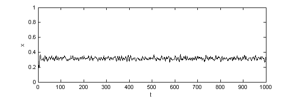
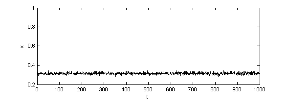
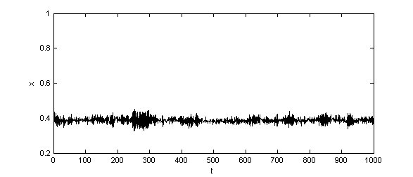
Figure 3. Time series of x with different values of S (a)S=0.01 (b)S=1 (c)S=1.99

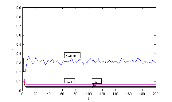
Figure 4. Time series of the ratios of cooperators when S<0, S=0 and S=0.01

3.5

There is a different kind of transition between the Chicken Game and the Benevolent Chicken Game around S=2. The transition gap is much larger than in the transition between Prisoners' Dilemma and Chicken Game. For all the cases, the gap remains the same as [2, 2.28]. Inside the gap the games behave like a Chicken Game, after the gap (when S>2.28) the oscillation continues with two major differences. The frequency seems to be the same for all later values of S for both the Benevolent Chicken and Leader Games. The amplitude has a decreasing tendency in S for the Benevolent Chicken Game but an increasing tendency in the Leader Game after some initial steps. These properties are illustrated in Figure 5, 6 and 7 with the values 0.1, 0.5 and 0.9 for x(0). We can also notice that there is no significant pattern change between the Benevolent Chicken and Leader Games. Three particular trajectories are shown in Figure 8 for x(0)=0.1 and S=2.3, 4 and 6 comparing the last two games.

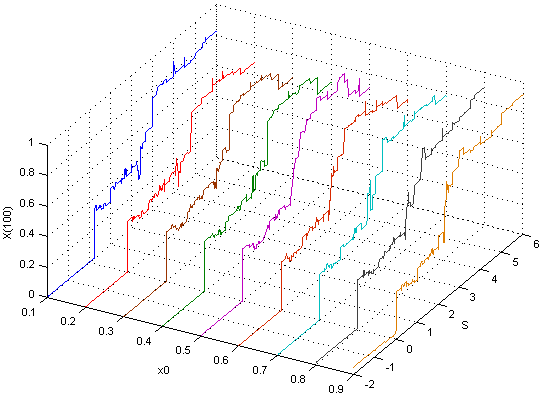
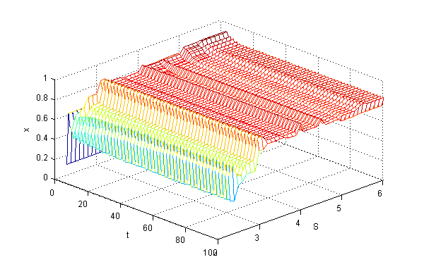
Figure 5. 3D plot of x as function of t and S, 2.3≤S≤6, x(0)=0.1

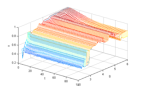
Figure 6. 3D plot of x as function of t and S, 2.3≤S≤6, x(0)=0.5

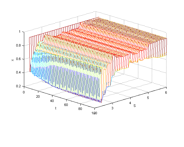
Figure 7. 3D plot of x as function of t and S, 2.3≤S≤6, x(0)=0.9

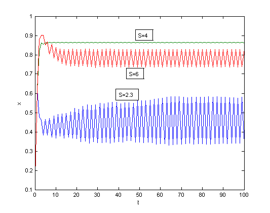
Figure 8. Comparison of time series patterns of x with different S values, x(0)=0.1

3.6

We have also performed the same series of computations by assuming that the agents do not consider themselves as members of their neighborhoods. In all cases we had very similar results to those presented earlier with the only difference that the boundaries between the different games slightly move up.

3.7

In the previous experiments we have assumed greedy agents, when changes in the behaviors of the agents were deterministic. We also repeated the computer study with Pavlovian agents. Here the behavior of each agent changes according to a well defined probabilistic rule. If P(t) denotes the probability of cooperation by a given agent at time t, then probability changes in time as:

(1)

While in the case of greedy agents all trajectories are deterministic, in the case of Pavlovian agents they are random, since the behavior of the agents is determined by the probability values (1). Each simulation can produce different trajectory, therefore we made 16 runs with identical P(0)=0.5 for all agents and computed the average values of the x(t) ratios for all t. If x*(t) denotes the "true" expectation and x_average(t) the average value computed from NS simulation runs, then from the Chebyshev inequality we know that with any ε>0,

(2)

where σ²(t) is the variance of the x(t) values. In our case σ²(t) was approximated by the sample variance, which was very small, less than 10^-6, since the different simulation runs were very similar. Notice that we had 10,000 agents, therefore, the relative frequencies were calculated from a very large sample size. The values of x(t) are then accurate for at least 2 decimal figures with 99.9% probability.

3.8

In the simulation we selected α=β=0.1. The trajectories for x(t) are very similar for all of the four games. Figure 9 summarizes the average trajectories for -2≤S≤6 and 0≤t≤50, from which a clear convergence can be noticed in all cases. It is also noticeable that the limit is increasing and very smooth in S.

Figure 9. 3D plot of x as function of t and S, agents are Pavlovian

Conclusions

4.1

In this paper we presented a first attempt of the systematic analysis of N-person finite neighborhood binary games. Linear payoff functions, C and D, were considered and it was assumed that they depend on the ratio of cooperators in the one-layer neighborhood of the agents. All agents were first assumed to be greedy. By fixing three parameters (D(0), D(1) and C(1)), the fourth parameter, C(0), was gradually increased giving transitions from Prisoners' Dilemma to Leader Game through Chicken and Benevolent Chicken games.

4.2

The largest change in trajectory patterns was observed between Prisoners' Dilemma and Chicken Game, almost no change between Benevolent Chicken and Leader Games, and a small change between Chicken and Benevolent Chicken Games. There was always a small interval of the varying parameter after the border line, in which the trajectory had the characteristics of the previous game. We could also observe how the properties of oscillating trajectories depend on the varying parameter value.

4.3

In this study we assumed that the agents consider themselves as members of their neighborhoods. We repeated the simulation study when the agents are excluded from their neighborhoods. Only slight differences could be observed in comparison to the previous case.

4.4

We also repeated the experiments with Pavlovian agents. There was no difference in the trajectory patterns, they always converged, and the limit changed as the model parameter was varied. This dependence was smooth and monotonic.

4.5

In this paper we considered and examined only a small portion of the possible cases of sensitivity analysis, when systematically varying parameter values change the type of the game and therefore the long-term evolution of the artificial society. We analyzed only the transition from Prisoner's Dilemma to Leader Game through Chicken and Benevolent Chicken games, however our future research will focus on examining the transitions between other game classes.

Acknowledgements

Sponsored by the U.S. Air Force Office of Scientific Research. Grant number: MURI Grant N00014-03-1-0510.

References

GUYER M J and Rapoport A (1969) Information Effects in Two Mixed Motive Games. Behavioral Science, 14. pp. 467-882.

HELBING D, Farkas I and Vicsek T (2000) Simulating Dynamical Features of Escape Panic. Nature, 407. pp. 487-490.

KITTS J A (1999) Structural Learning: Attraction and Conformity in Task-Oriented Groups. Computational & Mathematical Organization Theory, 5(2). pp. 129-145.

MERLONE U, Szidarovszky F and Szilagyi M N (2007) Finite Neighborhood Games with Binary Choices. Submitted to Mathematica Pannonica.

PANZARASA P, Jennings N R and Norman T J (2001) Social Mental Shaping: Modeling the Impact of Sociality on the Mental States of Autonomous Agents. Computational Intelligence, 17(4). pp. 738-782.

PANZARASA P and Jennings N R (2001) Social Influence and the Generation of Joint Mental Attitudes in Multi-agent Systems. Proceeding of the Eurosim Workshop on Simulating Organisational Processes, Delft, The Netherlands.

RAPOPORT A and Guyer M (1966) A Taxonomy of 2*2 Games. General Systems, 11. pp. 203-214.

SZILAGYI M N and Szilagyi Z C (2000) A Tool for Simulated Social Experiments. Simulation, 74. pp. 4-10.

SZILAGYI M N (2003) An Investigation of N-person Prisoners' Dilemmas. Complex Systems, 14. pp. 155-174.

SZILAGYI M N (2005) From Two-Person Games to Multi-Player Social Phenomena (in Hungarian). Beszelo, 10(6-7). pp. 88-98.

SZILAGYI M N (2007) Agent Based Simulation of the N-person Chicken Dilemma Game. In Jorgensen S, Quincampoix M and Vincent T L (Eds.) Advances in Dynamic Game Theory, Birkhauser: Boston. pp. 695-703.

ZHAO J, Szilagyi M N and Szidarovszky F (2007) A Continuous Model of N-Person Prisoners' Dilemma. Game Theory and Applications (in press).

ZIZZO D J (2006) You Are Not in My Boat: Common Fate and Discrimination Against Outgroup Members. Working Paper, School of Economics, University of East Anglia, Norwich, U.K.

Return to Contents of this issue

© Copyright Journal of Artificial Societies and Social Simulation, [2007]