©Copyright JASSS

JASSS logo ----

Stephen Wendel and Catherine Dibble (2007)

Dynamic Agent Compression

Journal of Artificial Societies and Social Simulation vol. 10, no. 2, 9
<https://www.jasss.org/10/2/9.html>

For information about citing this article, click here

Received: 01-Jan-2007    Accepted: 09-Jan-2007    Published: 31-Mar-2007

PDF version


* Abstract

We introduce a new method for processing agents in agent-based models that significantly improves the efficiency of certain models. Dynamic Agent Compression allows agents to shift in and out of a compressed state based on their changing levels of heterogeneity. Sets of homogeneous agents are stored in compact bins, making the model more efficient in its use of memory and computational cycles. Modelers can use this increased efficiency to speed up the execution times, to conserve memory, or to scale up the complexity or number of agents in their simulations. We describe in detail an implementation of Dynamic Agent Compression that is lossless, i.e., no model detail is discarded during the compression process. We also contrast lossless compression to lossy compression, which promises greater efficiency gains yet may introduce artifacts in model behavior. The advantages outweigh the overhead of Dynamic Agent Compression in models where agents are unevenly heterogeneous — where a set of highly heterogeneous agents are intermixed with numerous other agents that fall into broad internally homogeneous categories. Dynamic Agent Compression is not appropriate in models with few, exclusively complex, agents.

Keywords:
Agent-Based Modeling, Scaling, Homogeneity, Compression

* Introduction

1.1
This paper introduces a new method for processing agents in agent-based models that significantly improves the computational and memory efficiency of certain models. It accomplishes this by selectively compressing the agents' attributes, based on their changing levels of heterogeneity. The technique builds on the long tradition of compression in other fields and on the work on Stage et al. (1993) with respect to multi-scale agent-based models.

Considering Agent Attributes as Data

1.2
Compression algorithms are commonly used in a wide variety of applications that confront the layperson, from listening to digital music (e.g., the mp3 algorithm) to watching videos on DVD (e.g., the mpeg-2 algorithm). The concept is straightforward: compression algorithms find similarities or patterns in data and store that information in a more compact form. The compact form speeds up transfer times and makes it possible, for instance, to store a movie on a single DVD. John Cage's (in)famous composition 4'33", which consisted of 4 minutes and thirty-three seconds of silence, had a clear pattern — a long stretch of silence. It can be compressed into a trivially small representation.

1.3
Compression algorithms come in both lossless and lossy varieties. Lossless algorithms retain the integrity of the original data, so that absolutely no information is lost in the compression process. Lossless compression looks for perfect replicas of information, and replaces them with a tag that describes the replicated information and its extent. On the other hand, lossy algorithms combine similar pieces of information. The algorithm throws away a portion of the detail to create an even more compact form. A song may lose some of its nuanced tones, for example, or an image may lose some of its subtle shading.

1.4
Dynamic Agent Compression was developed out of the observation that in many models, agents are unevenly heterogeneous. While some agents are truly unique, a significant portion of the others may fall into a few broad internally homogeneous categories. In order words, there are patterns in the agents' data that can be stored in a more compact form through compression.

1.5
Dynamic Agent Compression is an extension of Stage et al.'s (1993) work on static agent compression, in which he used compression to tackle the problem of large-scale models with prohibitive resource requirements. His algorithm works as follows: Consider each agent as a point in a multi-dimensional attribute space with dimensions such as location, age, and health status. Find clusters of agents with similar attributes and replace them with aggregated agents. Assign the aggregated agent attributes that represent the core of the cluster and an expansion factor to represent the number of agents within the cluster. Use of these aggregated agents can save computational and memory resources either throughout the entire model or within expensive sub-models.

1.6
Where Stage et al. (1993) utilizes a once-off static compression of agents,[1] we propose a dynamic method that adapts to agents' changing heterogeneity during model execution. Moreover, we describe an extensible architecture where the individual modeler need only specify a limited set of parameters and where multiple compression algorithms (including Stage et al.'s (1993) COMPRESS algorithm) can be made available. These innovations lead to potentially much greater gains in efficiency and increase the potential scope of the algorithm's application. The initial concept is the same, however — treat agent attributes as data that can be compressed to ease the model's resource constraints.

Other Methods of Easing Resource Constraints in Agent-Based Models

1.7
In addition to Stage et al.'s (1993) COMPRESS algorithm, a number of related methods have been used to address the computational resource requirements of extremely large numbers of agents. As with Stage et al. (1993), many of the early efforts occurred in the ecology field as researchers modeled massive numbers of trees, fish, or bacteria. The most popular way of handling this problem is the Super Individual method (Scheffer et al. 1995), where a single agent in the model represents multiple entities in the real world such as bacteria. Rose et al. (1993), for example, employed a sampling and re-sampling algorithm to represent varying numbers of fish larvae, juveniles, and adults in his models. Hellweger and Kianirad (2006) recently expanded upon this literature with a location-specific method that addresses distortions caused by the scarcity of super agents in localized pockets of the model. Research into multi-scale models has also examined the creation of aggregate agents (e.g., Servat et al. 1998), but without the particular use of formal compression techniques.

1.8
Researchers have also sought to reduce constraints on their simulations by expanding the available resources. An obvious technique has been to purchase a sufficiently high-end machine or purchase compute-cycles on a high-end shared-use machine. Others have surpassed the resource constraints of a single CPU through parallel and distributed computing. Notably, the Los Alamos National Labs parallelized their agent-based simulation of transportation, TranSims (Nagel and Rickert 2001), by segmenting the geographical area under consideration and processing each segment on a different CPU. Unfortunately, decomposition is not feasible for all researchers due to a lack of expertise with parallelization techniques or the presence of complex interdependencies among agents in their models.

* Methodology

Overview

2.1
Dynamic Agent Compression is an efficient internal representation for groups of similar agents that adapts over time as the agents change their attributes. The key to Dynamic Agent Compression is that agents are compressed and decompressed as the simulation progresses, while the model interacts with all agents as if they were in a traditional agent-based environment. To accomplish this, Dynamic Agent Compression relies upon two components: a Compression Manager and a set of Agent Containers. The Compression Manager filters calls from the model to create, modify, and query agents, and passes them to the appropriate agent or Agent Container. Each Agent Container represents a cluster of similar or identical agents and holds a counter for the number of agents it contains.

2.2
Throughout the simulation, the Compression Manager handles the Dynamic Agent Compression process and frees the model from direct involvement in the details. At the start of the simulation, similar agents are grouped by the Compression Manager into Agent Containers while agents with particularly unique attributes are left ungrouped. During the simulation, the Compression Manager passes queries from the model to the uncompressed, individual agents and the Agent Containers. The Agent Containers in turn query the contained agents and monitor changes in their attributes. As agents differentiate themselves from their group, the Compression Manager extracts them from the Agent Containers and instantiates them as unique, individual agents. If uncompressed agents join an existing group of agents in attribute space, the Compression Manager adds them to an existing Agent Container or forms a new Agent Container. Under the supervision of the Compression Manager, Agent Containers behave like their component agents; they accept time ticks, can be visualized, can be check-pointed, and can answer queries from data collection probes. In each circumstance, they respond like a set of individually instantiated agents.

Calibration of the Compression Manager

2.3
As with other compression techniques, Dynamic Agent Compression can be implemented in a lossless or lossy manner and the user can set the desired level of compression. In lossless compression, only agents that are strictly identical from the perspective of model behavior are combined into a single entity. In lossy compression, similar agents are combined and the user specifies the degree of compression used, i.e., the degree of heterogeneity that the compression algorithm allows within clusters. Lossless compression provides an inexpensive way to make a model more efficient, but the efficiency gains are limited by the degree of heterogeneity in the model. Lossy compression discards information about the agents in pursuit of greater efficiency. Lossy compression can be applied to any agent-based model, but researchers must balance the efficiency gains against the potential for bias in model outcomes.[2]

2.4
In addition, the modeler can categorize agent attributes into three groups: compressible, state-dependent-compressible, and storable. Most numeric attributes should be marked as compressible, allowing the compression algorithm free reign to find patterns in the data. The modeler may know, however, that agents in certain states are likely to change frequently and thus should not be aggregated. These state variables should be labeled state-dependent-compressible, and the values corresponding to particular volatile states tagged to indicate that the agent should not be compressed when it is in those states. State-dependent-compressible variables, while necessary in these circumstances, should be otherwise avoided because they constrain the ability of the Compression Manager to find compressible categories of agents. Other attributes, such as agent names, do not directly affect model behavior but uniquely identify the agents. These attributes can be labeled storable, and the model will retain them within the container and assign them to agents as they decompress. Since the agents in the container are otherwise homogeneous, random selection from this list of stored attributes is functionally equivalent to random selection from the list of individual agents who originally had the stored attributes.

2.5
For illustration purposes, consider how agent attributes would be categorized in a simple model of agents foraging for food over a network. Agents in this model have three attributes: Name, Location, and HealthStatus. Location is compressible; otherwise identical agents can be compressed when they are located on the same node of the network or on sufficiently clustered nodes when lossy compression is used.[3] HealthStatus is an enumerated state variable that is state-dependent-compressible — hungry agents should never be compressed, because, in this simple model, hungry agents randomly move around the environment looking for food. Satiated agents will stay in place for a randomly determined period of time, and are compressible, i.e., they can be held in a single container at a location until a satiated agent randomly becomes hungry again or is otherwise activated and decompresses. Names are special in that when there are two satiated agents at the same location, i.e., that are otherwise identical in this simple model, it does not matter which identical agent has which name. Once one of the agents moves or changes health status, however, the name could be important; the agents' names must be stored during the compression process and retrieved upon decompression.

Sample Java Implementation

2.6
We implemented lossless Dynamic Agent Compression by adapting a previously developed sample model to use a generic Agent Compression library. We then customized the generic library with two model-specific extensions to test their impacts on performance. The Agent Compression Library contained an Agent Compression Manager and an Agent Container class which interacted with the model and agents via two simple class interfaces. These components functioned as follows:

2.7
The agent-creation process required minor modifications to the sample model. Calls to the Agents' constructors were replaced with calls to the Agent Compression Manager's agent creation function. The generic library included functionality to dynamically generate Agent Containers as individual agents were added to the model. In addition, we implemented an extension to the Agent Compression Manager that created empty Agent Containers for known categories during the initialization process, and filled them as the model sought to create new agents.

2.8
In the updated agent-creation process, the model would tell the Agent Compression Manager that it wanted to create each Agent based on a set of input parameters. The Compression Manager examined these parameters and either:

2.9
The main event loop of the model required similar changes to integrate the Dynamic Agent Compression library. Whenever the model called the Agents directly, we replaced those calls with calls to the equivalent function of the Agent Compression Manager. For example, at each time increment, the original model called its step function, which updated its internal information and then randomly activated each of the agents. We changed the model's step function to call the Agent Compression Manager's step function. Unbeknownst to the model, this function then called step on each unique Agent and on each Agent Container. The generic library provided functionality for the Agent Container to call the step function on its internal Compressible Agent once for each agent contained in the container. The first time it called the step function, it was a normal function call, unmodified from the Agent's normal procedure. The agent updated its internal information and interacted with the environment. The subsequent calls within the same time tick were timeless steps, where the Agent was asked simply to test for interaction with its environment but not update its internal information based on the passage of time. We implemented an extension to the generic library to take advantage of the statistical properties of the timeless steps of this sample model, and aggregate multiple timeless steps into a single random number draw.

2.10
In both the generic and customized versions, the Agent Container monitored its Compressible Agents it see if they changed attributes after they were activated. When they did change, the Agent Container extracted them from the container, and gave them to the Agent Compression Manager as individually instantiated Agents. The Agent Compression Manager checked the attributes of the newly-extracted Agents to see if they could join another existing Agent Container, trigger the formation of new Agent Containers, or remain as individually instantiated Agents.

2.11
When the model needed to gather information about the agents, for data-logging or other purposes, it similarly queried the Agent Compression Manager instead of the individual agents. As with the step function, the Agent Compression Manager queried the Agent Containers and the individual agents to gather the required information.

2.12
Figures 1 and 2 below illustrate the program execution flow of the model before and after adaptation for Dynamic Agent Compression, respectively.

Figure
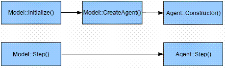
Figure 1. Program Execution Before Implementing Dynamic Agent Compression

Figure
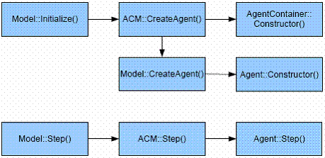
Figure 2. Program Execution After Implementing Dynamic Agent Compression (ACM = Agent Compression Manager)

* Sample Results

3.1
We tested the implementation of lossless Dynamic Agent Compression on the sample model and compared the model's execution time with and without compression. In this model, up to 5% of the agents were heterogeneous and uncompressed at a given instant and the remaining agents were categorizable and compressed. Agents transitioned frequently between the homogeneous and heterogeneous states; the set of heterogeneous agents completely turned over fifteen times during the simulation, making a majority of the agents heterogeneous and uncompressed at some point. The sample model was stochastic and simulations were run with ten random number seeds. While simulation outcomes varied from seed to seed, the time required to execute the model did not vary significantly.

3.2
Figure 3, below, gives the execution times for the sample model with and without Dynamic Agent Compression. With low numbers of agents (i.e., 100-500 agents, or 102-102.7 as in Figure 3), the overhead of Dynamic Agent Compression slowed down the model's total execution time slightly. As the number of agents increases (i.e., to 1,000-1,000,000 agents, or 103-106 as in Figure 3), both versions of the model showed increased execution times. The model with Dynamic Agent Compression, however, showed a significant improvement in efficiency over the normal model.

Figure
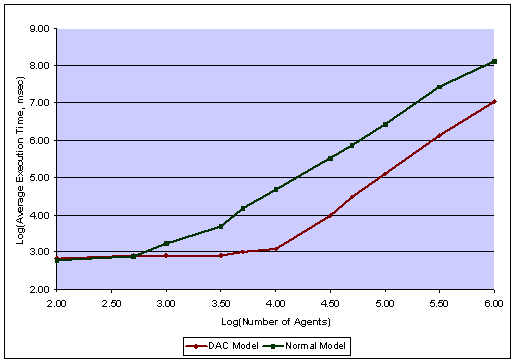
Figure 3. Execution Time of the Sample Model with and without Dynamic Agent Compression (DAC)

3.3
Figure 4, below, provides another perspective on the efficiency gains from Dynamic Agent Compression. Here, the relative speed of the model with Dynamic Agent Compression is given, as compared to the same model without compression. While improved efficiency from Dynamic Agent Compression was expected, the shape of the curve warrants some consideration. From our analysis of the execution logs, it appears that Dynamic Agent Compression begins to lose its edge over an uncompressed model as the number of agents passes a certain threshold and the model is too large to fit into memory even in its compressed state. Beyond this threshold, the application needs to write page files to the hard-drive, significantly increasing the overall runtime and diluting the gains from compression. As stated at the beginning of the article, Dynamic Agent Compression can reduce the resource constraints facing agent-based models; it cannot remove them altogether. Nonetheless, a 10× speed improvement for a 1,000,000 agent model is a notable accomplishment.

Figure
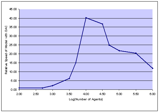
Figure 4. Relative Improvement in Execution Time due to Dynamic Agent Compression ( = Execution Time without Compression Divided by Execution Time with Compression)

3.4
We also found that model-specific customizations of the generic Dynamic Agent Compression library could have a noticeable impact on the model's performance. As noted above, we made two customizations: one to the initialization procedure to pre-generating Agent Containers, and another to the agent activation procedure within containers. The modification to the initialization procedure had no impact on model performance. The modification to agent activation provided a 30% improvement in efficiency, and illustrated the benefit of customizing Dynamic Agent Compression.

* Analysis

Gains from Dynamic Agent Compression

4.1
The computational gains from Dynamic Agent Compression will depend on the specifics of the model. A summary of that analysis is provided here, and a detailed discussion can be found in the Appendix.
  1. The time required to execute each tick t in a traditional agent-based model with N agents can be written as:

    Equation (1)

    Or the time to step each of the agents plus the time to step the rest of the model (graphics, data logging, control logic, etc.).

  2. With lossless compression, the time required to update the model on each tick can be broken down into the time required to step compressed and uncompressed agents and the time required to make transitions between these states (see Appendix for the derivation). Where:
    • N is the total number of agents in the simulation,
    • Ct is the number of Agent Containers at tick t,
    • at is the percentage of agents that are in a uncompressed state at the start of tick t,
    • bt is the percentage of compressed agents that are decompressed, i.e., become heterogeneous, during tick t, and
    • ct is the percent of uncompressed agents that are compressed, i.e., become homogeneous, during tick t,
    the formula for the time required to execute each tick becomes:

    Equation (2)

  3. When we simplify the equation by removing the relatively minor term for compressing agents,[4] and compare this function to that of a traditional model, Dynamic Agent Compression can be shown to improve the time required per tick of the model when:

    Equation (3)

    Or, equivalently: Dynamic Agent Compression improves the run-time efficiency of a model when the benefit from compression (the time required to step containers minus the cost that would have been incurred by stepping each of the agents within the containers individually) is greater than the cost of handling the flow of agents that decompress on each time tick.

  4. The relative speed of a Dynamic Agent Compression (DAC) implementation versus a traditional implementation can be expressed as:

    Equation (4)

  5. While the full equation is somewhat daunting (see Appendix), it has an important lesson: the relative speed improvement to be gained from Dynamic Agent Compression is bounded. If we consider the most extreme situation in which Dynamic Agent Compression completely eliminates the time required to handle agents, we can determine the upper bound on Dynamic Agent Compression's efficiency improvement with the following simplified equation:

    Equation (5)

  6. In a model where initialization took 0.1% of the total execution time, stepping the agents took 98.9% of the time, and stepping the rest of the model took 1% of the time, Dynamic Agent Compression would give a maximum improvement of 91×. In a model where initialization took 1% of the total execution time, stepping the agents took 94% of the time, and stepping the rest of the model took 5% of the time, Dynamic Agent Compression would give a maximum improvement of 17×.[5]
  7. Considering the lower bound on Dynamic Agent Compression's efficiency, it could theoretically slow down the total execution of the model when the initialization procedure (i.e., creating the Agent Containers and Agent Compression Manager) or the per-tick overhead (i.e., primarily the time required to decompress agents, as in Equation 3) exceed the total efficiency gains from handling compressed agents. Naturally, the modeler should not use Dynamic Agent Compression if it degrades performance.

4.2
In general, Dynamic Agent Compression is appropriate, i.e., the increased efficiency in agent storage outweighs the overhead of compression, in models where agents are unevenly heterogeneous — where a set of highly heterogeneous agents are intermixed with numerous other agents that fall into broad internally homogeneous categories. The greater the number of categorizable agents as a fraction of the total number of agents, the greater the potential gains from Dynamic Agent Compression. The more frequent the transitions of agents from compressed to uncompressed states, however, the smaller the gains. Sample applications include modeling the life-cycle of extremely large populations (e.g., fish-larvae or bacteria) or modeling the spread of ideas or diseases through a population. By compressing these otherwise homogeneous agents and handling updates to the compressed agents appropriately, the model can save significant computational cycles and memory resources without compromising the model's behavior.

Lossy Compression

4.3
While we have not discussed the implementation of lossy compression in detail here, a number of observations can be made. In terms of architecture, lossy compression is not fundamentally different from lossless compression. Instead of requiring that compression occur only when agents were identical, the Compression Manager would compress based on the clustering of agents in their multi-dimensional attribute space. It could perform a thorough analysis at the initialization of the model then use simpler cluster-boundary conditions to handle the compression and decompression of agents during the execution of the model, perhaps augmented by periodic re-analysis. The Compression Manager could use existing clustering algorithms for agent-attribute space (e.g., Stage et al. 1993) or implement new techniques.

4.4
While the architecture is straightforward, the benefits of lossy compression are much less clear. On the one hand, compression based on similarity instead of homogeneity would create more efficient representations of the agents. On the other hand, the cluster analysis process would require more overhead and the loss of detail would obviously affect model behavior. Much of the burden of addressing this problem rests with the clustering algorithm. A good clustering algorithm will maximize variation between clusters and minimize variation within clusters, thus minimizing the amount of agent detail it sacrifices. Clustering algorithms cannot guarantee, however, that the information they discard is unimportant to the model. At a basic level, the modeler can limit this distortion by decreasing the compression level, by flagging selected variables as state-dependent-compressible, or by choosing lossless compression. At a more advanced level, the modeler can customize the compression algorithm using detailed knowledge of the situation to avoid distortion.

4.5
While there may not be a way to completely eliminate the distortions caused by lossy Dynamic Agent Compression, there are methods to quantify and evaluate its effects. As with ordinary model parameters, those for Dynamic Agent Compression should be evaluated with a rigorous sensitivity analysis.[6] For example, in a Computational Laboratory setting (Dibble 2006), researchers could evaluate the effects of lossy compression on the model's behavior.

4.6
Nonetheless, it is important to put the consequences of lossy Dynamic Agent Compression in context. When lossy Agent Compression is not used (and lossless compression is not feasible), modelers of large-scale agent-based systems are often forced to manage resource requirements by decreasing the total number of simulations used in their study, decreasing the number of agents in their model, or using the common Super Individual approach (Scheffer et al. 1995). When researchers compensate for slower execution speeds by running fewer simulations, they sacrifice thorough and rigorous exploration of the model's behavior. Similarly, decreasing the number of agents in the model out of computational necessity risks having too few agents to elicit key effects, or otherwise distorting model behavior. Alternatively, the use of Super Individuals implicitly imposes a static agent compression regime without providing opportunities to evaluate the associated tradeoffs. Dynamic Agent Compression and Computational Laboratories support informed evaluation of the tradeoffs involved in the process.

Overuse of Scaling Techniques

4.7
A less obvious pitfall of Dynamic Agent Compression is that it can provide a tempting "solution" where none is needed. Many modelers naively presume that models require a strict one-to-one relationship between the number of agents in their model and the number of entities in the domain of study. In reality, many models do not require a one-to-one relationship because their behavior stabilizes after a certain number of agents are added to the population. Beyond this threshold the relevant characteristics of the system's behavior remain fundamentally unchanged or scale in an easily predictable manner. Using Dynamic Agent Compression or any other technique to unnecessarily scale a model up to a one-to-one relationship could waste programming effort, computational resources, and analysis time.

4.8
How is a modeler to know that the system stabilizes at a certain threshold of agents such that a one-to-one relationship is unnecessary? In some situations the only way to evaluate a model's sensitivity with respect to the number of agents is to take the model up to the full ideal number of agents and compare with results from the same model executed with fewer agents. In these cases, the modeler can use a simple generic implementation of Dynamic Agent Compression to test the model's behavior as the numbers of agents increases. If it turns out that the model requires the higher number of agents, then the modeler can customize Dynamic Agent Compression to improve its efficiency. If the higher numbers of agents are not necessary, then the generic Dynamic Agent Compression implementation has answered a valuable question, and saved resources for all future simulations.

* Conclusion

5.1
Dynamic Agent Compression can help agent-based modelers decrease the memory and computational resources required for certain models. We found that Dynamic Agent Compression allowed a sample one-million agent model to run in one tenth the time of the otherwise identical uncompressed model, with no impact on the model's behavior. In general, this approach is ideally suited for improving the efficiency and scalability of models in which a small number of unique agents co-exist with a larger number of agents that fall into internally homogeneous categories. We have also noted that a solid understanding of the operation of a model is advisable before endeavoring to scale a model up to incorporate extremely large numbers of agents. A generic Dynamic Agent Compression library, such as presented in this article, can help to evaluate the importance of such scaling.

5.2
Nonetheless, the discussion provided here is simply a beginning. Extensions could include a comprehensive analysis of the relative efficiency and tradeoffs of Dynamic Agent Compression versus alternative methods. We have briefly discussed the implications of lossy compression, but significant further research is needed before pursuing this perilous yet potentially rewarding path. Finally, the use of Dynamic Agent Compression in emergent multi-scale modeling seems especially promising.

* Acknowledgements

We would like to thank the Office of Naval Research, Grant N000140310062, for supporting this work. This paper expands upon a preliminary paper by Stephen Wendel and Catherine Dibble entitled "Dynamic Agent Compression" and presented at the Agent 2006 Conference "Social Agents: Results and Prospects," 21-23 September 2006, Chicago USA.


* Notes

1 Stage et al.'s (1993) process can be repeated for each execution of an expensive sub-model, but is nonetheless an inherently static method.

2 Bias in model behavior would be considered a compression artifact. As with any lossy compression technique, the goal is to provide modelers with the fewest artifacts for the desired level of compression. Artifacts can never be completely avoided, however, and the modeler should perform a thorough sensitivity analysis to evaluate tradeoffs.

3 The meaning of sufficiently clustered depends on the level of compression chosen. In a lossless implementation, agents would have to be on the same point in space. Lossless compression would be suitable for grid and network landscapes, but not for continuous real-valued landscapes. In a lossy compression, agents could be clustered if they were located in nearby points in space.

4 For example, compressing an agent in the sample implementation given above only entails incrementing the relevant Agent Container's counter and storing the agent's name in a list.

5 This is the maximum improvement if all else were constant; disk-paging and garbage collection issues can complicate the analysis. If the model is too large to fit into physical memory, and the computer is forced to use a page-file, then the simulation would run significantly slower. When Dynamic Agent Compression allows the computer to avoid paging, the realized gains would naturally be much higher.

6 Following similar robustness analyses that modelers already apply to input parameters, a la Steven Bankes's use of a Latin Hyber-cube to sample and analyze parameters (see www.evolvinglogic.com/el_news.html for an example).

7 A simple hash lookup can be used to see if they fit into an existing container.


* References

DIBBLE C. (2006) 'Computational Laboratories for Spatial Agent-Based Models'. In Leigh Tesfatsion and Kenneth L. Judd (Eds.) Handbook of Computational Economics, Volume 2: Agent-Based Computational Economics, Amsterdam: Elsevier/North-Holland, Chapter 31, pages 1511-1548.

HELLWEGER F. L. and Kianirad E. (2006) 'Spatially Explicit Individual-Based Modeling: Global vs. Local Fixed Agent Number Methods'. SwarmFest 2006 Presentation, June 2006, Notre Dame, Indiana.

NAGEL K. and Rickert M. (2001) 'Parallel implementation of the TRANSIMS micro-simulation'. Parallel Computing, 27(12):1611-1639.

ROSE K. A., Christensen S. W., and DeAngelis D. L. (1993) 'Individual-based modeling of populations with high mortality: A new method based on following a fixed number of model individuals'. Ecological Modelling 68(3-4):273-292.

SCHEFFER M., Baveco J. M., DeAngelis D. L., Rose K. A., and Nes E. H. (1995) 'Super-individuals a simple solution for modelling large populations on an individual basis'. Ecological Modelling 80(2):161-170.

SERVAT D., Perrier E., Treuil J. P., and Drogoul A. (1998) 'When Agents Emerge from Agents: Introducing Multi-scale Viewpoints in Multi-agent Simulations'. Lecture Notes in Computer Science 1534:183-198.

STAGE, A. R., Crookston N. L., and Monserud R. A. (1993) 'An aggregation algorithm for increasing the efficiency of population models'. Ecological Modelling 68(3-4):257-271.


* Appendix: Potential Time Gains From Lossless Dynamic Agent Compression

Initial Analysis

A.1
The time required to run any agent-based model can be divided into the time required for model initialization and the time required for model execution at each time step until the model's conclusion at time T:

Equation (1)

Dynamic Agent Compression is primarily designed to improve the execution time of the model at each time step, and will be the focus of the discussion here. Moreover, the initialization cost of lossless Dynamic Agent Compression as presented in the main paper is trivial.

A.2
The time required to execute each tick t in a traditional agent-based model with N agents can be written as:

Equation (2)

Or the time to step each of the agents plus the time to step the rest of the model (graphics, data logging, control logic, etc.).

A.3
In a model with Dynamic Agent Compression, the time required to step compressed and uncompressed agents and make transitions between these states can be considered separately:

Equation (3)

With terms:

  1. Time required to step the rest of the model
  2. Time to step the at% of the agents who are in an uncompressed state at the start of time t
  3. Time to step Ct containers holding (1- at)*N compressed agents at time t, including the time to check if agents should decompress
  4. Time to decompress bt% of the (1- at)*N compressed agents who become heterogeneous at time t
  5. Time to test the at * N uncompressed agents to check if they should compress at time t
  6. Time to compress ct% of the at*N uncompressed agents who become homogeneous at time t

A.4
For most Dynamic Agent Compression implementations, including the one used by the authors, we can make the simplifying assumption that the time required to compress an uncompressed agent is trivial, since the process only requires the storage of some unique information and the incrementing of a counter. In that case, Equation 3 simplifies to:

Equation (4)

With terms:

  1. Time required to step the rest of the model
  2. Time to step the at% of the agents who are in an uncompressed state at the start of time t
  3. Time to step Ct containers holding (1- at)*N compressed agents at time t, including the time to check if agents should decompress
  4. Time to decompress bt% of the (1- at)*N compressed agents who become heterogeneous at time t
  5. Time to test the at * N uncompressed agents to check if they should compress at time t

Specific Analysis of Lossless Dynamic Agent Compression

A.5
With lossless compression, it is trivial to test whether uncompressed agents should be compressed.[7] Thus, we are left with:

Equation (5)

With terms:

  1. Time required to step the rest of the model
  2. Time to step the at% of the agents who are in an uncompressed state at the start of time t
  3. Time to step Ct containers holding (1- at)*N compressed agents at time t, including the time to check if agents should decompress
  4. Time to decompress bt% of the (1- at)*N compressed agents who become heterogeneous at time t

A.6
Comparing this function with that of the traditional model from Equation 2, the time required per tick of the model is better with Dynamic Agent Compression if:

Equation (6a)

Or, equivalently,

Equation (6b)

I.e., when the time required to step the (1-at)*N agents compressed within containers plus the time required to decompress bt% of the compressed agents is less than the time it would have taken to just step the same number of uncompressed agents. Finally, we can restate this equation as:

Equation (6c)

Dynamic Agent Compression improves the run-time efficiency of a model when the benefit from compression (the time required to step containers minus the cost that would have been incurred by stepping each of the agents within the containers individually) is greater than the cost of handling the flow of agents that decompress and are instantiated as new individual agent on each time tick.

Relative Gains From Lossless Dynamic Agent Compression

A.7
The speed of a lossless Dynamic Agent Compress implementation relative to a traditional implementation is thus:

Equation (7)

A.8
Or, substituting Equations 2 and 5 into Equation 7,

Equation (8a)

See 4.1 for an analysis of these equations, including the upper and lower bound on efficiency to be expected from Dynamic Agent Compression.

Equation (8b)

----

ButtonReturn to Contents of this issue

© Copyright Journal of Artificial Societies and Social Simulation, [2007]