
Introduction
Agent-Based Modeling (ABM) and simulation are becoming increasingly common as a scientific method to examine complex phenomena (Bonabeau 2002; Epstein 2009; Grimm et al. 2005; Maglio, Sepulveda, & Mabry 2014; Thiele & Grimm 2015; Wilensky & Rand 2015). The value of ABM as a means for building theory and gaining a better understanding of mechanisms driving complex phenomena is becoming widely recognized. The computational nature of these models allows them to be run frequently (with varying parameters), making ABM a particularly useful tool for exploring the parameter space of dimensions that drive the phenomena under study, and conducting computational experiments on the impact of changes in these dimensions.
This ability of ABM to explore a large parameter space makes it a valuable tool for decision-making and policy development. ABM’s ability to examine both impact at local and higher systems level makes it increasingly used as a decision support tool in complex social systems. When using ABMs to guide decision-making and policy development, it becomes critical to ensure that these models accurately capture the nuances of the phenomenon, so that their behavior becomes increasingly realistic, and they can be used to make predictions about the phenomenon in practice.
We classify the resulting models as high-fidelity models, and loosely define them as being more inclusive and detailed, incorporating a higher number of dimensions, being strongly grounded in empirical data, with model behavior that produces realistic behavior when compared to observed data, all with the aim of supporting decision making. In contrast to Janssen (2009) who identifies two types of models, we identity a spectrum for models ranging from completely abstract to including many elements and in greater detail based on empirical data, without a clear cut-off as to when exactly models become high-fidelity. Models aimed at highlighting the dependence relationships, so-called theory-driven models, reside towards the abstract side of this spectrum. Whereas high-fidelity models are placed closer to the real-world side. As high-fidelity models aim to support decision making in practice, for them to be useful one will need to demonstrate that these models produce realistic findings by validating model behavior against empirical data. Only when validity is shown one can use the models to make accurate projections and support decision making.
The relatively high number of (interacting) mechanisms in high-fidelity models make it challenging to associate the system-level behavior, which is generally used as a source for validation of model behavior, to the behavior of underlying mechanisms. This means that to ensure the model behaves as intended, we need to validate each mechanism (and module capturing that mechanism) individually as well as their interactions with other, related mechanisms. This makes accurate replication of high-fidelity models more laborious, to such an extent that we propose that it requires a different set of replication and documentation strategies as compared to those presented in the current replication literature. Thus, there is a significant gap in our scientific protocols for the process of replicating high-fidelity ABMs.
Our paper aims to fill this gap by providing best practices distinct for replication of high-fidelity models, and highlight which practices are shared with research focused on replicating theory-generating models (e.g. Wilensky & Rand 2007; Rand & Rust 2011; Fachada & Rosa 2017). Specifically, in this paper, we address two fundamental questions. First, what are successful approaches, procedures, and practices for replicating high-fidelity models? And second, what can those who build high-fidelity models do to facilitate replication of their models?
To address these questions, we report on our efforts in replicating a modeling research study conducted by Jenness and colleagues (Jenness et al. 2016). In this study, a network-based model of HIV transmission dynamics, parameterized with empirical data on sexual partnership network structure, sexual behaviors within partnerships, and HIV transmission risks given sexual activity, was used to evaluate different scenarios of scaling up of HIV Preexposure Prophylaxis (PrEP) among men who have sex with men (MSM) in the United States. PrEP is a highly effective preventive medication, which has to date seen limited use among those who could benefit. We undertook this replication effort with the goal to verify and validate both the study results and underlying model behaviors.
The remainder of this paper will be structured as follows. First, we will discuss the value of replication and review the existing literature on replication of ABMs. We will identify facilitators and barriers, and consider how high-fidelity model replication fits within the current literature. Second, we provide a brief overview of the study being replicated and the original model, which from this point onwards we will refer to as EpiModel, in line with the name of the platform on which the original model was built (Jenness, Goodreau & Morris 2018). Next, we highlight the replication process, resulting in the replicated model, which we from this point onwards will refer to as the NetLogo HIV spread model (the NHS model) (Hjorth, Vermeer & Wilensky 2018), using three separate examples of our replication process. Each example focuses on a specific module at a different level of granularity. And lastly, in our discussion section, we present a synthesis across the lessons we learned during replication and provide general guidance for effective replication of high-fidelity models.
The Value of Replication
Replication is a fundamental building block of scientific practice. By checking if others who follow the same methods can obtain similar results, the reliability of these results can be increased, and previous research can be used as the foundation for future experiments, facilitating the building of scientific knowledge.
Similar to improving the validity of research outcomes, replication can improve the validity of computational model outcomes, yet doing so requires two additional steps (Wilensky & Rand 2007; Rand & Rust 2011). First, as computational models are by definition abstractions of the real world, their conceptual model — which describes how the various (agent) behaviors and interactions with the environment occur — will need to be checked. This process is called model validation, and refers to the process of checking whether the model captures a phenomenon accurately enough to answer the driving question behind the model (e.g., “Does the model behave like the phenomenon observed in the real world?”). Second, the implemented model — the translation of the conceptual model into actual code— needs to be considered. This process is called model verification and refers to the process of checking that the translation from conceptual model to the implemented model is correct (e.g., “Does the model do what it is intended to do?”). Both of these processes should occur naturally during replication of ABMs and other computational models (Wilensky & Rand 2007; 2015, Rand & Rust 2011) before the implemented model can be considered as credibly producing counterfactual evidence of experiments for hypothesis testing, and decision-making. The fact that complex systems models often exhibit sensitive dependence to initial conditions (Lorenz 1972), with very small changes in inputs sometimes resulting in very large differences in outputs, leads to challenges in conducting these model correctness checking processes.
Replication of ABMs
Several computational modelers have previously recognized the need for model replication (Axtell et al. 1996; Edmonds & Hales 2003; Wilensky & Rand 2007; Thiele & Grimm 2015). Wilensky and Rand (2007; Wilensky & Rand 2015), for example, focused on standards for replicating ABMs and provided an overview of the replication work done in the agent-based domain prior to 2007; this includes the seminal works of Axtell et al. (1996) and Edmonds & Hales (2003). We highlight Axtell et al. (1996) specifically as they introduce three standards of replication (RS) used in our work: numerical identity — the notion that exact numerical matching across multiple implemented models is obtained — distributional equivalence — the notion that two models produce distributions of results that cannot be differentiated statistically — and relational alignment, the notion that two models can be shown to produce the same internal relationship among their results. These standards highlight that, depending on the output that is considered, varying levels of strictness can be adopted in what one considers successful replication, with numerical identity being the strictest, followed by distributional equivalence and relational alignment respectively. We note that choosing a stricter standard does not imply a more rigorous replication — a high quality replication will choose a replication standard that is well matched with validation of the focal model and outcomes. If, for example, we are replicating a model of network partnership formation which aims to produce variations of a partnership network, it would not be wise to use an RS of numerical identity as by its very nature the original model must produce a distribution of partnership networks, and therefore a RS of distributional equivalence would be preferred.
Since the Wilensky & Rand (2007) paper, work on replication of ABMs has continued. Merlone, Sonnessa, & Terna (2008) compared three implementations of a model of industrial production to study the emergence of structures found in the real world. They found relational but not numerical alignment among their models, and recognized that the affordances of the platform used to implement the model mattered strongly for simulation results. Will & Hegselmann (2008) reported on their failure to replicate a trust model that aims to describe the formation of markets, based on the original publication by Macy & Sato (2002). Janssen (2009), presents a replication of the Artificial Anasazi model (Axtell et al. 2002) which considers historical population dynamics in the Long House Valley in Arizona between 800 and 1350. While they find results that relationally align with data, they conclude the original findings hold only partially and are produced mainly by fitting the model to field data. Stonedahl & Wilensky (2010) and Gunaratne & Garibay (2017) build replications of the same model showing how generic algorithms can be used for calibration and optimization models. They show this method can be leveraged to present alternative theories for observed behavior. Radax & Rengs (2010) replicated the Demographic Prisoner's Dilemma model (Epstein 1998), and found that the replicated model results differed from the original, and distributional alignment could only be achieved under certain circumstances. They highlighted timing in the models as a potential cause of the discrepancies. Arifin & Zhou (2010) described the replication of an Anopheles gambiae mosquito’s model using multiple implementations. The model simulated population dynamics based on a conceptual framework of reproductions and death. The authors found that variations among implementations had an extensive effect on population structure and dynamics. Miodownika et al. (2010) replicated the Bhavnani (2003) model that considers the process by which historical political units could have evolved to form civic regions that approximate those observed in present day Italy. The authors were not able to distributionally align the implemented models, and noted that observed differences in model outcomes might stem from implementation differences. Seagren (2015) replicated the model of Tiebout sorting (Kollman et al. 1997), which considered the stylized interactions between individual (political) preferences and local policy making under various electoral landscapes. The authors achieved relational alignment in their replication, and highlighted the value of doing additional sensitivity analysis based on the replicated model. Donkin et al. (2017) replicated a model originally published by Potting et al. (2005), describing an agro-ecological world in which pest insect’s behavior was modeled on two platforms. The authors based their replications solely on the published model, and found model behaviors to be numerically, distributionally and relationally dissimilar. They attributed this misalignment, to a large extent, to the unavailability of source code. Fachada & Rosa (2017) replicated a version of the predator–prey model, and used it as a showcase for formal testing of replication and model alignment, resulting in guidelines on how to examine replication efforts statistically. The above presented review of replication efforts shows how difficult it has been to fully reproduce model-based research, sometimes even at the least strict level of relational alignment.
The limited degree of alignment achieved in many replication studies is both problematic, and highlights the importance of replication as a means to ensure reliable models and validated model outcomes. Without undertaking model validation and model verification, reliability of models and their outcomes are questionable. With the trend of models to become more sophisticated and become widely adopted, a lack of a comprehensive replication methodology and practice would have the potential to result in a strong increase in unreliable models. In turn, the field of simulation modeling runs the risk of lowering its credibility and risking the integrity of computational modeling as a rigorous scientific method.
This risk has been previously identified (Edmonds & Hales 2003), and others have highlighted various lessons for improving replication efforts. Wilensky & Rand (2007), for example emphasize the need for replication standards, availability of detailed documentation including source code, and the value of interaction and collaboration with original authors. Thiele & Grimm (2015) identify a number of ways in which to stimulate a culture of replication within the research community, including, standardizing model descriptions, software platforms, and sub-models, and providing open code and documentation. Additionally, various authors have argued for the need for standards, both in terms of model description (Grimm et al. 2006; Grimm et al. 2010; Grimm et al. 2017) model building (Grimm et al. 2014), and sharing (Collins et al. 2015). Furthermore, recent work by Fachada & Rosa (2017) describes a set of formal testing approaches for replication. This body of work on replications has identified several standards that help integrate replication into general modelling practice and ABM usage. While these are certainly steps in the right direction, sufficient documentation of replications remains relatively rare.
Replication of high-fidelity models
The provided overview of replication work done within the ABM domain, consists largely of theory-driven models built without extensive calibration based on existent empirical data. The purpose of these models is generally to help researchers better understand either the underlying mechanisms that drive a complex phenomenon, or to generate or improve their theory of the phenomenon. By design, the models used in such attempts are more stylized, focus on behaviors that are more abstract, and have a limited connection to the complexities present in real world phenomena. While such simplifications are what makes these models especially powerful for theory development and for eliminating possible explanatory factors, not all models have those specific aims.
In contrast, the high-fidelity models aim to support decision-making and policy development. High-fidelity models embrace the complexities of real-world complex systems to make model outputs as relevant as possible and maximize their value for decision support. Models with these aims will thus incorporate a large number of dimensions and will use empirical data to link with the real-world dynamics. As such, they will have a larger number of moving parts which are likely to be interdependent. Such interdependencies make it challenging to fully grasp how the system-level behavior traces back to the behavior of modules within the overall model. This means that unless we validate each mechanism (and module) individually, even numerical identity on the model level could be the result of a coincidence (albeit an unlikely one).
To our knowledge, there is a void in the documentation on replication of high-fidelity models. Yet, the increased complexity of these model suggests that accurate replication of high-fidelity models is more laborious, to such an extent that it requires a set of replication strategies different from those documented in previous replication literature, a hypothesis we explore in this paper.
The Computational Experiment Being Replicated
In this paper, we describe the replication of a simulation study by Jenness et al. (2016). The primary focus that study was to predict the impact of CDC’s recommendations for HIV Pre-Exposure Prophylaxis (PrEP) among men who have sex with men (MSM) in the United States. This biomedical intervention, when taken regularly by MSM engaged in unprotected anal intercourse in non-monogamous relationships, greatly reduced the risk of HIV infection for this high-risk group (Liu et al. 2016). However, to date, PrEP usage in the United States is far below that recommended by the Centers for Disease Control and Prevention (CDC 2014).
To judge the impact of the CDC guidelines, Jenness and colleagues developed a network-based model of HIV transmission dynamics, calibrated with empirical data on sexual partnership network structure, sexual behaviors within partnerships, and HIV transmission risks given sexual activity. The resulting EpiModel (Jenness et al. 2018) was the platform used to evaluate different scenarios of scaling up PrEP based on different interpretations of CDC guidelines. As these indications for PrEP require an interpretation that could be implemented in practice, e.g., a non-monogamous relationship cannot be completely assessed during testing of only one partner, multiple versions of the CDC guidelines were defined and their impact on population-level infections averted were compared (see Table 1, Jenness et al. 2016). This paper aims to replicate this experiment and consequently validate the results of the same nine different interpretations of the CDC’s indications for PrEP, and doing so required two replication steps.
In the first step, based on the conceptual model of HIV transmission used in the original study, an implemented replication model had to be created, which we call the NetLogo HIV spread model (the NHS model) (Hjorth et al. 2020). We opted to build the NHS model using a platform other than the original EpiModel for two reasons. First, being able to replicate successfully across platforms makes the results more robust. Second, as building high-fidelity models requires a high level of familiarity with the platform in which the model is build, we chose to adopt the platform the replicators were most familiar with. The EpiModel has been implemented in the open source R package similarly called EpiModel, the version used was version 1.2.5 (Jenness et al. 2018) and this package relies on a statistical estimation of dynamic networks (exponential random graphs modeling, ERGMs) to form and dissolve sexual relationships. The replication model uses NetLogo version 6.1. NetLogo is a widely used and flexible ABM platform (Wilensky 1999), and our implementation forms network structures based on agents’ local behaviors. Consequently, the NHS model followed a conceptual model for governing the network formation and dissolution that is similar, but not identical, to the one used in the EpiModel. For all other parts of the model (behavioral dynamics, and transmission risks) the NHS model does strictly follow the conceptual model from EpiModel.
In the second step, once the NHS model was built, we repeated the computational experiment originally done with EpiModel with the re-implemented NHS model, and compared the results of this replication to the original. In doing so, we simultaneously attempted to validate the results of these experiments and the conclusions in the original study.
EpiModel — A brief overview of the conceptual model
EpiModel incorporates a wide array of dimensions feeding into system level HIV transmission behavior. The behaviors of these dimensions are anchored in empirical data from various sources to ensure the model behavior matches observations made of the phenomenon in practice. As such, EpiModel clearly fits our description of a high-fidelity model both in terms of its model and its goals.
Below, we provide an overview of the original model. We consider it essential when considering any replication study that the original model description be accessible, and consequently we refer the reader to the Technical Information of the original study (Jenness et al. 2016) for full details on the description of the EpiModel method, and the model itself, and its component behaviors. Additionally, we refer the reader to the complete source code for EpiModel which is publicly available on Github (http://github.com/statnet/EpiModelHIV). Here in this paper we present a minimal overview of model behavior below, and an abstract flow of the stages of the model behavior can be found in Appendix A.
EpiModel by default consists of two main components: a partnership dynamics component and a transmission behavioral component. The partnership dynamics component determines how agents create and break sexual partnerships with each other over time, forming longer or shorter-term relationships and one-time ties. The transmission behavioral component describes the spread of HIV based on the behavior of agents within this sexual activity network, how they choose to have intercourse, sexual positions, condom use, etc. Together, these two components simulate how HIV spreads dynamically in this MSM population. For the purpose of the specific experiment in the original paper an additional component describing the various PrEP intervention interpretations is added to this model. While the model combines the interactions between these components into system level dynamics, each of these components acts and can be described relatively independently.
Partnership dynamics: The modeled partner network described three types of partners: main partners, shorter-term casual partners with repeated contacts, and one-time partners. Parameters for sexual behavior were drawn from 2 empirical studies of MSM in Atlanta, Georgia (Hernández-Romieu et al. 2015). The predictors of partnership formation varied by partnership type, with different model terms for degree (number of ongoing partners for each member of the pair), age, homophily (selecting partners of similar age and race/ethnicity), and sexual role segregation (such that 2 exclusively receptive men cannot pair, nor can 2 exclusively insertive men). For main and casual partnerships, there was a constant risk of relationship dissolution, reflecting the median duration of each type. This resulted in a dynamic network on which HIV can spread.
Transmission behavior: Per-act factors influencing the transmission probability for HIV included viral load of the infected partner (Hughes et al. 2012), condom use (Weller & Davis‐Beaty 2002), receptive versus insertive sexual position (Goodreau et al. 2012), circumcision for an insertive negative partner (Wiysonge et al. 2011), and the presence of the CCR5-\(\Delta\)32 genetic allele in the HIV negative partner (Marmor et al. 2001; Zimmerman et al. 1997). Once infected the clinical HIV progression was programmed to follow the empirical courses of disease and antiretroviral therapy (ART) treatment profiles (Mugavero et al. 2013). ART is associated with a dramatically decreased viral load and consequently lower transmission risks (Cohen et al. 2011) and extended life span (Goodreau et al. 2014). Persons who were HIV positive and not on ART were modeled with evolving HIV viral loads that changed their infectivity over time. After infection, persons were assigned into clinical care trajectories controlling for timing of HIV diagnosis, ART initiation, and HIV viral suppression, to match empirical estimates of the prevalence of these states (Sullivan et al. 2015).
PrEP Indications and Uptake: The CDC guidelines for PrEP prescription consider the sexual behaviors in the 6 months prior to diagnostic HIV testing (the risk window). MSM were assessed for PrEP indications only at visits in which their HIV test result was negative, as ART, rather than PrEP, is indicated for positives. At time of HIV testing, eligible MSM were allowed to start PrEP only if the proportion of MSM on this regimen had not surpassed a threshold coverage of 40% of the population. This threshold accounted for an external constraint on PrEP availability, and was varied in robustness checks in the original experiment.
PrEP eligibility is determined based on the 3 behavioral conditions in the CDC guidelines: Unprotected Anal Intercourse (UAI) in monogamous partnerships with a partner not recently tested negative for HIV, UAI outside a monogamous partnership, and AI in a known-serodiscordant partnership (CDC 2014). For each criteria 2 different functional definitions were implemented: a “literal” version based on the specific guideline wording and a “clinical” version that could be more realistically assessed in practice.
An important goal of the simulation was to order the alternative interpretations of CDC guidelines on their ability to effect incidence. While the clinical versions are generally less strict than literal ones (e.g., a monogamous individual may erroneously indicate his partner is also monogamous), no version is defined in such a way to be superior to any other. Thus, all orderings are possible, and therefore their replication would provide a good test of distributional or relational alignment.
The Replication Process in Overview
The full replication process constituted several months of work spread out over a period of 18 months. In it we followed an approach that can be divided into three stages. In the first stage, the replicating team started from the published documentation to validate the translation from conceptual model to implemented model, and used the Technical Information from the original paper to implement the NHS model based solely on this information. As this translation left some open questions as to how to implement the NHS model, the second stage involved connecting with the senior author of the original model to provide clarification on the model implementation details. In the third stage, we started testing the alignment of the models, one module at a time, at which point we pulled in the full source code to further align the NHS model.
While all three stages are critical for effective replication, in this manuscript we report primarily on the third stage of our process. Rather than going through each step of the replication process we will highlight the process by presenting three examples of replication that occurred during out process: the replication of the viral load progression module, the replication of the transmission risk module, and the replication of the computational experiment. The selection of these specific examples is based on four reasons. First, each of the examples considers replication at a different level of granularity, the first example considers a micro-level module, the second a meso-level module consisting of a combination of multiple modules, and the latter the full system-level behavior of the model including all its sub-modules. As such, the combination of examples provides insight into how interactions among modules occurs and can cause emergent behaviors, and how the hierarchical structure and modularity can be leveraged during replication. Second, this combined set of examples allows us to highlight how the replication differed from the original and discuss challenges during replication (Wilensky & Rand 2007). Examples of such challenges include the impact of having a different set of authors replicate the model and interpret model documentation, the potential impact of differences in algorithms, and the impact of varying the platform and/or modeling philosophy can have. Third, each of the examples considers replication using a different replication standard (Axtell et al. 1996), therefore the combination of examples allows us to provide a comprehensive description of replication covering each of these standards. Lastly, we found the combination of these three examples to be illustrative of the lessons we learned during our process of replication of this high-fidelity model, and as such this set of examples was considered both necessary and sufficient for the purposes of this manuscript. In the sections following, we will describe each of the examples in detail.
Example 1: The Viral load module
The first example involves replication of the viral-load module. We chose this example specifically because the viral load of a person with HIV directly affects their risk of transmitting HIV. Consequently, it is considered a critical component in determining the system level spread of HIV. While being a critical driver of systemic behavior, viral load progression is a dimension that can be specified relatively independent of the remainder of the model and hence is an ideal starting point for replication. When someone contracts HIV, “viral load” is used as a measurement of the number of copies of the virus that person has in their blood; it is directly related to infectivity. Detailed viral load progression for HIV in the absence of ART follows four general stages. In the first stage upon infection (the acute rise stage) the viral load will rapidly increase to a peak viral load, after which the viral load will drop towards set point levels (acute decline), this stage is followed by a relatively long period of stable viral load (stable set point), until inevitably in the AIDS stage the viral load increases until mortality (Little et al. 1999).
The structure of the original viral-load module
EpiModel captures the evolution of HIV viral load continuously. Following the previously described viral dynamics it determines an individual’s viral load based on two dimensions; disease stage, and anti-retroviral treatment (ART) adherence.
Disease stage: The progression of viral load over the course of an infection is captured using four stages in EpiModel: 1) An initial rapid increase to peak viral load, 2) a rapid decline from peak to set-point viral load, 3) a long period of stable set-point viral load, and 4) an AIDS phase with increasing viral load and eventual mortality. Both within and between stages the rate of change over time was assumed to be linear.
ART: An infected individual can be put on anti-retroviral treatment (ART) when their test for HIV results in a positive test result. ART treatment will effectively reduce the set-point viral load of the individual (for as long as they remain on ART). The extent to which this set-point is reduced depends on individual attributes (suppression level), and the extent to which viral load is effectively reduced depends on the sustained adherence to ART.
The process of replicating the viral-load module
Replicating the viral progression module from EpiModel required various steps and substantial effort on the replicators’ part. In the following paragraphs we will highlight the process we went through to align this module across implementations, this process is strongly influenced by the framework put forward in Wilensky & Rand (2007).
The first step in any replication process, is to determine which sources of information are going to be used during replication. Replication can be based on various types of model descriptions: a fully documented model description, a model’s source code, or a verbal description of the model during communication by the model authors. Each of these descriptions has its own affordances and limitations, and requirements in terms of access to resources. We initiated our replication process by considering only the model description, and did so for two reasons. First, the model description is aimed to be comprehensive, and as such should be a source that is both detailed and relatively easy to process. Second, for most researchers, the documentation is the (only) source that is available for replication, and as such replicating based on the documentation is a good representation of what one can reasonably expect to achieve in replication based on the current reporting standards.
With our replication source determined, we considered the level of alignment that is desirable and required to consider the replication effort successful. This applies as much to the replication of complete models as it does to sub-modules. Among the three standards of replication, relational alignment, distributional equivalence and numerical identity (Axtell et al. 1996), we selected numerical identity as the replication standard for the viral load module for three reasons. First, we see viral load to be a critical component of EpiModel as it is one of the most prominent factors driving the risk of transmission. Second, high accuracy in the replication is critical for alignment of results on the system level. Values of viral load can vary by six orders of magnitude depending on the stage of infection. Thus, we considered it necessary to adopt a strict replication standard that would allow us to capture such fluctuations accurately. Third, as viral load describes an agent property (which is independent of population behaviors), and there are substantial quantitative data on which to build a model of viral load, it was feasible to numerically align this module. These arguments indicated numerical identity was both an achievable and desirable replication standard.
Next, we determined the mechanisms that went into the viral load calculations, and identified for which cases alignment of model behavior needed to be tested. We explored three behaviors: 1) the viral load progression in the absence of treatment, 2) the dynamics of getting on and off ART, and 3) the interaction between the viral-load progression and the treatment behavior.
While studying the viral progression in the absence of treatment we found that even minor implementation differences in implementation can have large effects on model behavior. Conceptually we know that viral load numbers, the number of copies of the virus present in a ml of someone’s blood, impacts the risks of transmission of HIV; the more virus in one’s blood the higher the risk of transmission. The implemented EpiModel determines the extent of this effect on risk based on the following calculation: \(2.45^{(x-4.5)}\) where \(X\) is the logarithm (base 10) of the number of copies in one’s blood. For each of the stages of infection, the documentation described end point viral load, and it described a linear change over time across the various disease levels. EpiModel applied this linear effect to the logarithm of the viral load levels (so effectively increasing \(X\) linearly), while our replication applied a linear change over time to the number of virus copies in one’s blood. While this might seem like a minor difference in interpretation, the effect this had on emergent model behavior was significant, with the NHS yielding an HIV prevalence level of \(\sim\)10% higher than the EpiModel implementation.
To understand the impact on the system level better, the actual viral load across implementations needs to be plotted, and the interactions of the viral load with other modules needs to be understood. Note that the two implementations differ only in the way they process changes in viral load, and consequently only produce different results in the stages of the infection during which viral-load is in flux (acute rise, acute decline (which we combine into an onset stage) and the AIDS stage). For both implementations the viral load level during these stages are plotted in Figure 1.
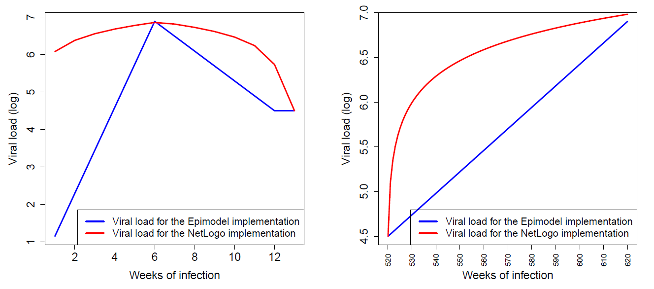
While differences are observable across implementations, the gravity of their impact can only be understood within the larger model structure. To do so we first reiterate that log of viral load is used as an exponent in the risk calculation formula \(2.45^{(x-4.5)}\). This implies that even small differences in the log of the viral load (\(X\)) will have substantial impact on the actual risks of transmission during phases where \(X\) is high. Add to this the notion that during the onset period (acute rise and acute decline) the infection is acute and is consequently much more contagious (by a factor 6), and one can see how risks of transmission can be drastically inflated by a seemingly small implementation difference.
Figure 2 shows the factors by which risk of transmission are inflated during the onset and AIDS stages based on only the viral-load and acute stage multiplier. A detailed look at these results (Appendix B) shows that the difference of implementation yielded an inflation by on average a factor 12.509 during onset, 2.258 during the AIDS stage and 1.442 over the entirety of the infection. These numbers highlight how interaction between modules can radically amplify minor implementation differences, and in turn affect the emergent behaviors on the system level. In our case the interaction yielded a situation of extremely high risk after initially contracting HIV, which caused a self-perpetuating mechanism of new infections.
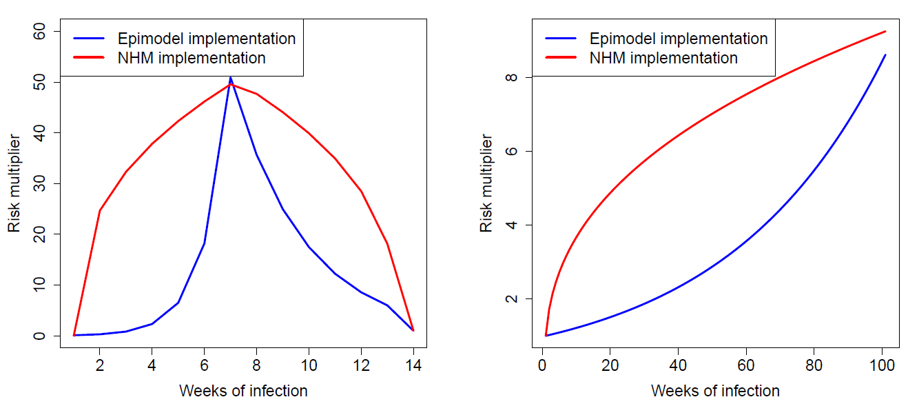
We should note that both implementations are accurate translations from the conceptual model, which posited linear changes over time, and hence from a model verification standpoint there is no a priori reason to prefer one over the other. This is a perfect example of how seemingly small differences in implemented models, even when using the same conceptual model, can have significant impact on the emergent properties of a system. The complex nature of high fidelity models stems from to the interactions and feedback loops inherent in them, so that small changes can be amplified to have significant effects on the system level behavior. This observation highlights that even minor differences in implementation can potentially result in large changes in model behavior on the system level, and that further attention to the behavior of this module is needed to understand its behavior.
The progression over time of viral load in EpiModel is based on previous work by Little et al. (1999). Taking their progression as the ground truth for HIV viral load progression, we can compare the behavior of both implementations to the behavior in that paper as a means to validate the behavior of both implementations. The second figure in Little et al. (1999) reveals a smooth transition of viral load progression which more closely fits the implementation of the NHS model than it does the EpiModel. Regardless, we choose to align the NHS model to the implementation of EpiModel, to ensure comparison of these models. But in doing so we note that our replication effort reveals that the viral load progression module is an area where future model improvements might be desirable.
For successful replication, it proved critical that we also aligned the treatment dynamics. In implementing the process of ART adherence in the NHS model, we based our modeling decisions primarily on the provided documentation. However, in the case of treatment dynamics, the extensive documentation (EpiModel has an elaborate 25 page description of model behaviors (SI of Jenness et al. 2016) did not provide sufficient information for exact re-implementation of the module. We consider this to be an inherent problem with documentation of high-fidelity models rather than an issue with EpiModel specifically, as the sheer amounts of documentation and translation needed in this type of model is likely to introduce points of uncertainty.
To clarify the sections that were unclear to the replicators during the re-implementation process, the replicating team contacted the lead author of the EpiModel (SMJ), to engage in a richer means of communication regarding model functioning. Based on a concrete set of clarifying questions, the author of EpiModel referred us to specific segments of the source code of EpiModel specifically addressing these questions (see Appendix C). Taking into consideration the sources code allowed the replicating team to strictly align the behavior of the treatment module in the NHS model with EpiModel. This process is a clear example of how each resource has different affordances when it comes to replication, the documentation provides the main conceptual model, the authors the details and the model overview, and the source code the details needed for re-implementation.
With both the natural progression and impact of ART treatment modules evaluated on their own, we considered the interaction between the two. Effectively we considered the effect of initiating or maintaining treatment at different stages of the disease progression. Being on ART for a week has an effect of reducing the viral load by a given amount (up until a given threshold). Similarly, not adhering will result in the agent moving back towards the default trajectory. As ART effects wear off during the AIDS stage, such dynamics result in a set of six scenarios (see below) for which the behavior will need to be tested for alignment.
- Get on ART during acute rise stage, and remain on ART
- Get on ART during acute decline stage, and remain on ART
- Get on ART during stable setpoint stage, and remain on ART
- Being on ART during acute rise stage, and go off ART during that stage
- Being on ART during acute decline stage, and go off ART during that stage
- Being on ART during stable setpoint stage, and go off ART during that stage
This set of scenarios was replicated for 2 types of agents (those with complete suppression, and those with partial suppression), resulting in a total of 12 critical scenarios. The effects of treatment are fairly straightforward during the set-point viral progression stage (scenarios 3 and 6) as the viral load in that stage is stable except for deviations due to ART treatment thus leaving very little room for variation in interpretation of how to implement. However, during the other stages, the effects of treatment are far less obvious. As viral load is changing naturally during these stages, the implementation of an additional change is far from unambiguous.
To test alignment we wrote test cases for all of the 6 scenarios both in EpiModel, by extending its code, and the NHS model. We then compared the outputs of these test scenarios across implementations. In doing so, we observed some model behavior which was not expected based on the conceptual model. We found that in EpiModel once a single dose of ART is taken, the default trajectory is disregarded and viral load progression is based on an in-treatment (and potentially adhering) logic rather than the traditional viral progression path. Particularly in the acute rise (and decline) stages, this can yield a dramatic shift from default behavior (see Appendix D), in which taking one pill can effectively prevent the occurrence of the complete acute stage, or slow down the default viral load decline to such levels that it is worse than not taking a dose at all (when a dose is taken during the acute decline stage).
The replicating team considered these scenarios to be unrealistic, but recognize that they will occur extremely rarely. Similar to the earlier variation in implementation, they also found that these scenarios do have a substantial effect on the virility of an individual and that such discrepancies are amplified during the acute stage, and consequently significantly impacted the system level behavior of the model. This is another example of the value of replication as a tool for model validation. It is unlikely anyone would first explore, second notice, and third interpret, the impact of such an implementation decision unless replication was attempted.
The viral load progression module proved difficult to replicate primarily due to a difference in the conceptual model of the ART module between the two teams. More specifically, the assumptions relating to the role of path dependence in this module differed between the original model builders and the replicators, which caused an initial hurdle in alignment. Where EpiModel effectively made an agent’s viral load a Markov process conditional on the previous state, the replicating team assumed that path played a role in determining these treatment dynamics. In the path dependent interpretation, it is not only the state but also the direction in which the viral load has moved in the past that determines the effect of a dose of treatment. E.g., the effects of treatment might be very different for someone whose viral load has been on the rise and is currently at \(10^5\) compared to someone who has a viral load that has been dropping and is currently at \(10^5\). Capturing such a conceptual interpretation of treatment requires the path an agent has taken to get to its current state, and the history of agents’ behavior, to be incorporated into the model, whereas the Markov implementation does not incorporate such information.
While our goal was to numerically align behavior of the module across implementations, the replicating team decided to adjust its initial implementation in the NHS model, and re-implement it so it would strictly follow the implementation of EpiModel, while at the same time marking modeling of ART effects as an area that deserves future considerations in sensitivity analysis. Consequently, the NHS model dynamics were modeled to effectively stating that once a dose of treatment is consumed an individual’s viral-load will change with a rate of 0.25, and will gravitate towards the set-point viral-load (4.5) with that rate when no treatment is consumed, similarly it will gravitate towards the virally suppressed level of viral-load (1.5) with that rate when treatment is consumed. This is in line with what EpiModel implementation does. Once this conceptualization was implemented both implementations indeed showed numerical identical results for the viral-load progression module, and hence replication of the viral-load module was considered successful and numerically identical (see Appendix E).
Example 2: replication of the risk-of-transmission module
As a second example of our replication process, we discuss the replication of the module that determines the risk of HIV transmission. This module describes the transmission of HIV by means of a process that depends on both a series of agent behaviors and on the complex evolution of sexual activity networks in the model. We chose to report on this module as it differs from the previous module in some key dimensions. First, this module considers the behavior of a dyad rather than an individual, and hence considers interactions among agents. Second, this module includes randomness, whereas the previous module was fully deterministic. Third, the module consists of multiple sub-modules, that each feed into it, as such it highlights the relevance of hierarchy, structure and interaction among sub-modules during model replication. And lastly, this example presents a perspective on how to deal with situations in which strict alignment in one of the sub-modules is impossible (or as in our case purposely foregone).
The structure of the risk-of-transmission module
The risk-of-transmission module can be conceptually broken down into a set of three independent (sub)modules that, when combined, determine the risk of spread on the system level. 1) A Partnership Formation and Dissolution Module, which determines where ties are present to facilitate spread using three types of ties, main, casual and one-time ties; 2) a module determining the rate of sexual acts within each tie; and 3) a module determining the Risks of Transmission per sex act.
The process of replicating the risk-of-transmission module
Replication of the risk-of-transmission module was done using an approach that began similar to the one described for the viral-load example but differed in later steps. We again considered each of the sub-modules in isolation, before combining them into to a more complex module where they interact, which is similar as before. However, as one of the sub-modules differed across implementations our assessment of the interactions of these modules differed. During the replication process we made the conscious choice to not to strictly replicate the partnership formation and dissolution sub-module. We did so primarily because the philosophy of network formation adopted in EpiModel differed from our own. EpiModel adopts an ERGM based formation process which bases the formation of ties on the fit with system-wide structural characteristic. In contrast, the replicated model assumes partnership formation to inherently occur at the individual level, where individual decision making results in an emergent structure. Consequently, to align with this modeling philosophy, we implement this module in NHS in a classic agent-based manner, where each individual’s partnering decisions result in an emergent partner network (see Appendix F for pseudo code of this module). We do use the global properties to cap individual’s behaviors to ensure the formed networks in the NHS model match the global properties of those produced by EpiModel. In choosing a different conceptualization for producing aggregate network structures and dynamics our replication has become a test of the hypothesis that these two different approaches to partnership formation align, not only in the requisite aggregate parameters, but rather align well enough to support model validity and the main conclusions of a successful replication. We stay alert to the possibility that this hypothesis will be rejected and these different mechanisms will yield fundamentally different results.
While partnership selection is one of the sub-modules that affects the risk of transmission, our design choice has implications for the method of replication and the replication standard adopted. As one of the input sub-modules conceptually differs, aiming for numerical identical results at the level of the complete module makes little sense. In fact, to consider alignment when the various sub-modules are combined, we will need to first control for the effects of the partnership formation and dissolution module and test alignment for all other interacting sub-modules. Only after that process is done can we include it in our tests for alignment and see if this specific sub-module yields comparable results. As such, we add an intermittent step in our replication process, in which after aligning the sub-models individually we check for their interaction while controlling for the partnership formation and dissolution module.
Aligning the risks per act sub-module
The first sub-module, the per-act risk of transmission module, has 5 independent inputs. The first, the Viral load module, has been discussed previously, two others are trivial binary checks. The acute stage and CCR-5 mutation each have their own risk multiplier. Two less obvious interacting sub-modules include condom use and sex-role.
All of these input modules are fully deterministic, and consequently we consider numerical identity an appropriate standard for replication for this module. Additionally, as these per act risks are the backbone of the spreading behaviors we consider accuracy critical for overall model behavior, and hence claim that numerical identity for this sub-module is desirable.
For the two remaining non-trivial input modules we identify the variability that can occur given that all other inputs remain constant. Ceteris paribus, sexual acts resulting in HIV transmission can occur in three ways; An HIV-positive agent can either be insertive, receptive, or versatile (i.e. both positions), and whose behavior is conditional on the sexual behavior preferences of both partners in the tie. When versatile behavior occurs, it is considered a compound of 1x insertive and 1 x receptive act, and consequently by knowing both the risk for the insertive and receptive acts, one can deduce the risk related to versatile acts. As such, 2 critical states exist from the sexual behavior perspective. From the condom use perspective also two options are available — Protected and Unprotected — resulting in a total of 4 (2 x 2) critical scenarios for which alignment has to be tested.
For both the EpiModel and NHS models we create scripts to generate the risks based on these critical input scenarios and compare results across models. We initially found significant differences across implementation, which required substantial effort to identify — a difference in interpreting a parameter being on a log versus a log-odds scale — and then minimal effort to resolve. (Details on the steps required for alignment of this sub-module can be found in Appendix G).
Aligning the rate of sexual acts per partnership sub-module
Next, we considered the sub-module that determines the rate of sexual acts within a partnership. Note that the rates in this module are based on average behaviors in a previous cohort study (Hernández-Romieu et al. 2015). These rates thus represent the mean behavior within the entire population, stratified by partnership type. Based on the population behavior each individual relationship in each week is assigned an activity by drawing from an independent Poisson distribution. This means that stochasticity is added to this module’s outputs. While one could potentially align the random number generators and random seeds across both implementations — and by doing so attempt to obtain numerically identical results-- we consider this a task that requires too much effort for relatively little gain. Instead we adopted the less strict replication standard of distributional equivalence, which is more appropriate, allowing us to incorporate the stochasticity and consider the alignment in a distribution of outputs rather than every unique outcome.
Comparing the number of acts per type of tie across both models initially revealed large differences. More specifically, the replicated model showed far less sexual activity across all types of ties. Exploration of the potential causes of these differences proved difficult, and only after inspection of the EpiModel source code were we able to pinpoint the cause of the misalignment. Differences were caused by an inflation factor applied in EpiModel, which was not implemented in the NHS model. EpiModel included a parameter (AI_Scale), which modified the number of acts in all types of ties; it was used to fit the model’s system level HIV prevalence to observed empirical data. In the implemented EpiModel study this value was set at 1.324, effectively inflating the sexual activity by that factor across the board (compared to empirical point estimates). Incorporating this inflation factor in the NHS model resulted in distributional equivalence of acts among implementations (see Appendix H).
Aligning the partnership formation and dissolution sub-module
As mentioned prior, in building the NHS model a design choice was made not to strictly follow the network formation and dissolution processes as implemented in EpiModel. In EpiModel, the network formation and dissolution is controlled by a statistical model for network structure: a temporal exponential random graph model (TERGM) (Krivitsky & Handcock 2014). TERGMs try to find dyadic mechanisms that results in a fit of a set of system-level network structural properties; as such it makes local behaviors conditional on population level properties. Such a process runs somewhat counter to the modeling philosophy of agent-based models in which agents use only local information in their decision making and have no access to population-level information. While implementing a network formation module that strictly follows the EpiModel method would be possible in NetLogo, such a module is not as good a fit for ABM, as ERGM models fit aggregate model parameters. Instead we decided to re-implement the network formation process in a more agent-based fashion, and replaced the TERGMs network component by an individual-level matching module that similarly fits the population distributions, but does so by employing local matching decisions for partner selection and dissolution (See Appendix F).
Controlling for the partnership formation and dissolution module
As, by design, the network formation process differs across implementations, it is reasonable to assume the networks created with those processes will differ. Both implementations form networks with the same number of individuals, density, and degree distribution, and hence produce networks with similar global network parameters (SI of Jenness et. Al. 2016) for a detailed parameterization). However, the networks formed are likely to differ locally as the mechanisms that determine where ties are formed differs drastically. As it is known that such a local difference can have a large impact on spreading processes, it is to be expected that HIV spread will differ in the networks formed using the different implementations. Consequently, should we find any difference in the spread module we would be unable to attribute to these differences to any failed alignment in specific mechanism or module or interactions among them; observed differences might stem from variation in the partnership network formation, the dynamics of network change, or misalignment elsewhere in the module, making for an inconclusive test scenario. To effectively compare model implementations, we therefore needed to control for network formation (and its dynamics) while testing alignment of the interaction of the two other modules.
Leveraging the modular structure of both models, we could relatively easily do so. The network module simply provides an input (a network structure, and list of agent states) to the spreading module. As such, we can swap out the module in both implementations with a fixed network having stable characteristics. As long as the stable network is identical as across both models, the stochastic behavior on top of this network should be the same as long as the models’ behavior is in fact aligned. To create such a test, we ported the world-state across models: we outputted all the agent and tie attribute data of a given world state from EpiModel and wrote a script to read those into the NHS model, creating two identical instances. By matching the world-state across both models we ensure both are identical in terms of the networks they use, as such we control for the influence of network structure. However as network are dynamic and change over time the network structures will only stay identical for a single time step (tick). To control for the dynamics of the network we consequently consider only the spreading behavior in the first tick (when networks are still identical), and do a test for alignment for those spreading data. This “one-tick-test” effectively controls for modules known to vary across implementations and isolates the modules and mechanisms that we do want to align. In modular models this general approach can be extremely powerful to reduce the complexity, and allow one to focus on alignment of specific (sets of) modules. What is more, this type of test can be devised for formally testing higher level modules even when lower sub-modules are known to deviate. In our case as the network formation and dissolution was modified purposely this test was our primary tool for aligning the spreading behavioral component across implementations.
A “one-tick-test” for aligning the spreading module
During the one-tick-test, we evaluated alignment of the system-wide transmission risk by considering the number of new infections across implementations, the HIV incidence. Note that the occurrence of new incidence cases is conditional upon a set of stochastic processes throughout the system. This has two implications on how alignment needs to be tested; 1) To obtain reliable results we need a sufficient number of repetitions of the same experiment to account for variance that is inherent in any stochastic process, and 2) the stochasticity implies that the results are unlikely to be numerically identical, and that we instead will look for statistically similar results, and adopt distributional equivalence as the replication standard.
In both implementations we found substantial variance of the incidence across repetitions with new incidences cases ranging from 0 to 18 per time step with a mode of 4. Given the relatively low per act transmission risk, such variance is not surprising. We can assess this variance by repeating the same experiment multiple times and considering the average behaviors across these repetitions. Effectively we are producing a distribution of incidence, which becomes more and more stable as behavior is averaged over more repetitions. We found that our incidence distribution becomes stable once the number of repetitions was increased to the order of 50-100k, and that consequently the variance of the mean incidence largely disappeared as that point, and that very narrow confidence intervals for the incidence distribution are obtained. Consequently, we used the one-tick-test with 100k repetitions to compare the incidence across implementation for a given world-state. This comparison revealed distributional differences in incidence across the implementations, given that we had previously aligned the sub-modules that drive this distribution this was a surprising result.
Addressing the misalignment across spreading modules
After finding differences in the mean values of transmission risks across implementations, we explored the module for indications of the source of misalignment. First, we looked at the mean risks for each tie individually (over 50k repetitions). We fixed the number of acts per tie to one (for all tie types), and compared the risks obtained across both implementations. We filtered out the ties that yielded different mean risks across implementations and explored their characteristics to identify the potential source of the differences. We went through several iterations of this process, which allowed us to 1) spot a bug in our script for porting world-states across implementation, which caused two agent attributed to be switched, 2) notice that the acute stage had been renamed in a later version of EpiModel which resulted in it not being correctly translated during the porting across implementations resulting in a misalignment of risks, and 3) most notably, it allowed us to track differences back to a discrepancy in the risk calculation module, which we will further elaborate on below. These are but a few examples of how statistical testing of alignment can serve as an exploratory tool for finding source of misalignment.
By outputting the distribution of risks for each tie (rather than just the means), we observed that a total of up to six different risks could be generated within a given tie. These risks are linked to the critical scenarios identified previously as a combination of the sexual behaviors (insertive/receptive/versatile) and use of condoms (Yes/No), resulting in \(\times\) \(=\) 6 scenarios. We found that for the versatile sex acts, the risk numbers across the implementations did not align. Note that such sex acts are the compound of both an insertive and a receptive sex act, and hence had previously been considered a non-critical scenario in our tests. However, due to differences in the way risks were compounded, the NHS model and EpiModel did not yield the same numbers after compounding, even when the risk for the individual insertive and receptive acts did match numerically. Changing the implementation of compounding of risks in the NHS model (effectively treating the act as two separate acts one insertive and one receptive rather that combining them in a single chance of success) resulted in numbers for all risk scenarios that matched exactly (achieving numerically identical results also for versatile events). After these changes, the one-tick test showed promising results, with nearly identical HIV incidence frequency distributions across implementations, when simulated 100,000 times (Figure 3).
Diagnostic plots and tests for distributional alignment
While the overlay of the two distributions in Figure 3 seems to show a high degree of agreement as the frequencies look similar, this type of figure is a poor way to determine distributional differences since there is little room to examine the tails of the distribution. In what follows, we describe the statistical tests and plots we used to compare distributions of new incident cases across implementations.

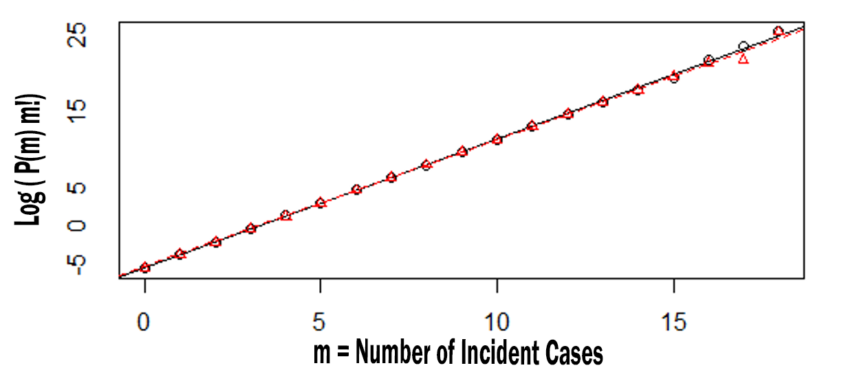
We examined whether the new incidence distributions in both implementations match well against a Poisson or mixture of Poisson distributions. This is shown in Figure 3, where for each observed number of incident cases, \(k= 0, 1,\dots K\), we plot this against a function of the following observed proportion, \(P(k)\) of observed cases across all simulations. With \(Y(k) = \log (P(k) + \log (k!)\), a Poisson random variable will show a linear relationship on \(k\), with intercept \(–\lambda\) and slope \(\log \lambda\), where \(\lambda\) is the mean of the distribution. A typical Poisson mixture distribution will show an approximate quadratic relationship. In this plot, both the EpiModel and NHS model plots look exceptionally linear, and they are nearly on top of one another. Thus, there is no indication of a departure from Poissonness, and the difference in the EpiModel and NHS model means are extremely small.
These graphical results were then repeated across 50 variations of randomly generated starting networks. A Poisson model fits all these data well (and formal tests for extra-Poisson variation are all nonsignificant). Consequently, we conducted formal tests of the differences between EpiModel and NHS model means under a Poisson assumption.
Running this formal test on all 50 networks revealed that, for 10 out of the 50 networks (20%), there was a significant difference in mean incidence rates between the EpiModel and the NHS model at the 0.05 level (Appendix I). This is far above the 2-3 out of 50 trials we would expect by chance, signaling that full alignment had not yet been achieved. Our analysis also revealed the differences in means across implementations were tiny in terms of effect sizes, with the largest being 0.006, indicating that a small but systematic difference was occurring.
To address this misalignment, we once more looked at the distribution of risks per tie and found (as established before) that the transmission risks calculated are identical across the models. This left only two potential sources of the discrepancy: 1) the frequency of acts that occur is different across the implementations, or 2) the distribution of risk scenarios — that is, a combination of using a condom, and choosing a sex-role which is associated with a set risk of transmission — is different across implementations. Outputting data of all acts (per tie) revealed no structural differences across implementations in the distribution of the risk scenarios. For the rate of sex acts, we only found significant differences in one type of sexual tie — Casual Ties — but not for the others. After observing these results, we found that the parameter for the mean number of sex acts in casual ties differed slightly between the EpiModel code — 0.955 — and the value reported in its documentation — 0.96 —, the latter being the rounded up version of the prior. Whereas the prior was used in the EpiModel implementation, the NHS model, relying on the documentation, used the latter.
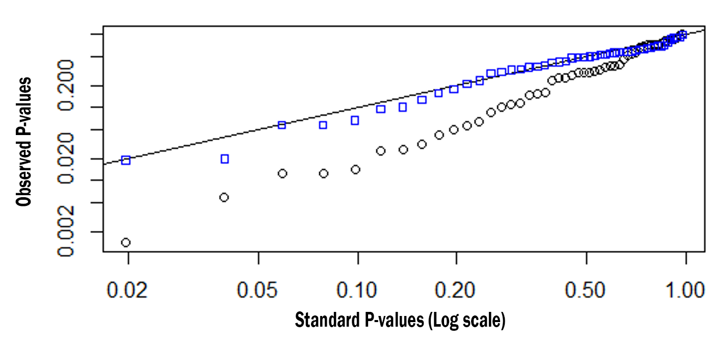
We adjusted the EpiModel implementation to reflect the value used in its documentation (and the NHS model) and reran the one-tick test. The results (Appendix I) showed that in 48/50 (96%) of cases, the outcomes of the models were statistically indistinguishable. Figure 5 shows two sets of significance levels for these tests; the lower set for 50 variations using the initial parameter, and the upper ones for the same 50 variations using the updated (aligned) parameter. On the x-axis we provide the expected values of 50 p-values (log transformed) under a null distribution; on the y-axis are the ordered observed p-values.
Under the null distribution, the p-values should fall along the \(y = x\) line. The observed p-values for the EpiModel and the NHS model comparisons with the non-adjusted parameter (black squares) fall well below this line, evidencing systematic differences between these EpiModel and the NHS model distributions. However, once the parameter for mean number of casual sex-acts was aligned to 0.955 (blue squares), the p-values fall nearly perfectly on the \(y = x\) line, indicating excellent agreement.
Figure 5 describes how small a difference we are able to detect. This empirical quantile-quantile (EQQ) plot (Chambers 2018) uses the ordered corrected effect sizes of EpiModel versus the NHS model on the x-axis, and presents the ordered effect sizes for the non-aligned variations on the y-axis. The non-aligned version clearly deviated from the expected \(y = x\) line. The marginal distributions for the corrected and rounded-off effect sizes are shown on the top and right sides of the figure, and the medians are shown on the dotted lines. Note that the median for those that are corrected are centered at zero while the median for those with the rounded off parameter are slightly positive. Also note that the effect sizes are all exceptionally small, ranging from +/-0.005, demonstrating how precise we can estimate these quantities with large enough number of simulations.
Example 3: Replication of the computational experiment
Generally speaking, high-fidelity models are created with the aim of making inferences about certain phenomena. They serve as a tool for facilitating experimentation or exploration, and as such increase our knowledge and support decision making. EpiModel is no exception in this regard. In the work by Jenness et al. (2016) the model is used to make inferences about the relative effectiveness of different interpretations of CDC clinical practice guidelines of PrEP indications among MSM, effectively determining what the criteria are for being eligible to receive PrEP. By adding a PrEP intervention module to the previously described transmission risk module, the effects of various interpretations are studied using a computational experiment. Because this experiment effectively incorporates the full model, we chose this computational experiment as our final example of replication.
The experiment compared a total of 10 scenarios; 1 baseline without interventions and 9 variations with different (combinations of) interpretations of CDC guidelines for PrEP. For each scenario a period of 520 time-steps (representing 10 years) was modeled, after which the prevalence was recorder. As each simulation run consists of a multitude of stochastic decisions which have an inherent path dependence in them, random fluctuation in model behavior are to be expected. Consequently, obtaining reliable results for any given scenario will require averaging the results across multiple repetitions. For this reason each of these scenarios was repeated 250 times. Based on the collected data, a the mean incidence, and a 95% confidence interval of this mean is calculated for each scenario, allowing a comparison of the relative effectiveness of the interpretations of the CDC PrEP guidelines. Additionally, as data for the EpiModel experiment is presented in Jenness et al. (2016), this also allowed us to compare the NHS model findings to the findings of EpiModel.
Prior to running the experiment, EpiModel implemented a burn-in procedure to generate a randomized starting state. During the burn-in process 250 instantiations of the model (set up with the parameters reported) were run for a period of 2600 time-steps (50 years). This burn-in period aimed to make sure that bias from the initial setup was dissolved and potential model dynamics stemming from a potentially biased setup had stabilized and as such played no role in the experiment. After this burn-in period, the single instance (1 out of 250) that best fitted empirical data (indicated by a stable prevalence at a level of \(\sim\)26%) was selected. This “world” was then used as the starting state of all experiments.
The structure of the computational experiment
In replicating this experiment, there are three modules that needed to be considered; the intervention module, the partnership selection module, and the transmission module. These modules essentially make up the complete EpiModel method, and determine the macro-level behavior of the model. Two of the modules (partner selection and transmission risk) have been discussed as part of our previous replication examples. In order to compare CDC guidelines, only a module describing the effects of such guidelines had to be added to the model.
Intervention Module: This module effectively describes how individuals get tested, and, when found to be HIV-negative, get assigned to PrEP if eligible. The assignment to PrEP depends on two factors; 1) an individual’s indications, which depend on interpretation of the CDC guidelines being adopted, and 2) on availability for PrEP. The latter we kept fixed for the purpose of replication as we consider it of secondary importance in our replication efforts. Once an individual is on PrEP, their risk of being infected is reduced by an amount which is conditional on the level of adherence to the drug.
The process of replicating the experiment
Replication of the intervention module proved particularly challenging. The documentation, which provided a plain English description of the meaning of the interpretations of the CDC guidelines, proved insufficient to convey and distinguish the nuances of how each of these interventions varied across scenario, and hence how it should be implemented. Communicating with the senior author of EpiModel model did resolve many but not all issues in this regard, the nuances of the interpretation are simply hard to convey in plain English. However, by referring to specific sections of the source code directly, the EpiModel author made sure these nuances and the differences in the meanings of the various intervention scenarios could be distinguished.
In replicating the experiment, we opted for relational alignment for two reasons; first, relational alignment suffices to answer the key question. In the original paper the experimental results are discussed only in relative terms (A is more effective than B) and the actual numerical impact is ignored (e.g. A reduces prevalence by X percent). The authors of the original experiment made this choice intentionally, and this signals the relative confidence in the models numerical results. More specifically, it indicates that the relative orderings are considered the most critical take-aways from the experiment, especially among those that produce the lowest incidence. As such, relational alignment, as a replication standard, suffices for making claims about the alignment of these results across implementations. Second, we consider it feasible, in fact the only feasible standard available. The fact that by design the partnership selection and dissolution module differs across implementations, and the fact that the resulting differences in structure can have an impact on the spreading dynamics (Vermeer et al. 2018), limits the alignment that can be expected among the two models. Based on these difference we consider the chance that models will produce outputs that are numerically identical essentially non-existent, and the chance that results distributionally align slim at best. Consequently, it is most appropriate to aim for a replication standard of relational alignment.
After having aligned the intervention module based on the source code, we ran a set of simulations with varying conditions for qualifying for PrEP, replicating the experiment conducted in the original study (see Table 1). Note that in these simulations we know that the spreading behavior module is aligned, and that partnership selection module is not strictly aligned.
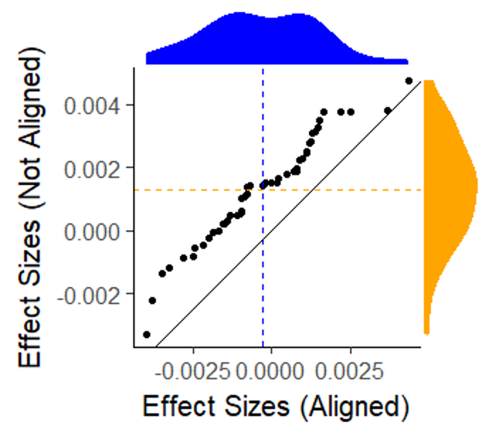
The results of these simulations (Table 1, Figure 6) revealed three critical things. First, our results show that we are quite far from distributional alignment. A comparison of the 10 means yields a z-value of 8.6, with a p-value \(< 10^{-17}\). Second, there is a very strong correlation across implementations (Figure 6), in fact the correlation between the average incidence in the 10 scenarios, across EpiModel and the NHS model was 0.98. And third, in addressing the question of whether the orderings of the 10 EpiModel and 10 NHS model interventions on incidence are similar, we find that 92% of all pairwise orderings in intervention effectiveness were consistent across implementations. We note that this percent could well be improved if the EpiModel means had higher precision like those we calculated in the NHS model (Table 1 ).
| Criteria code | Interpretation of the CDC guideline for prescribing PrEP | EpiModel | NHS model |
| Baseline | 25.9 | 25.3 | |
| Condition 1: Unprotected Anal Intercourse (UAI) in a monogamous partnerships with unknown HIV status | |||
| 1a | A partnership is monogamous when it is the only tie for both partners | 24.5 | 23.1 |
| 1b | A partnership is monogamous when it is the only tie for at least one of the partners | 23.6 | 21.6 |
| Condition 2: Unprotected Anal Intercourse (UAI) outside a monogamous partnership | |||
| 2a | Any tie beyond the first classifies as ‘outside a monogamous partnership’. | 23.3 | 20 |
| 2b | All ties other than the main tie is classify as ‘outside a monogamous partnership’. | 21.1 | 15.7 |
| Condition 3: Anal intercourse (AI) in any known-serodiscordant partnership | |||
| 3a | Any AI will quality the person | 23 | 20.8 |
| 3b | Only Unprotected AI will qualify the person | 23.5 | 21.7 |
| Combinations of conditions | |||
| J1 | Criteria 1a, 2a and 3a all quality an individual | 20.6 | 16.2 |
| J2 | Criteria 1b, 2b and 3a all quality an individual | 19.2 | 14.8 |
| J3 | Criteria 1b, 2b and 3b all quality an individual | 19.4 | 14.9 |

Discussion
Wilensky & Rand (2007) have specified 6 different dimensions in which replications can vary from the original model: (1) time, (2) hardware, (3) languages, (4) toolkits, (5) algorithms and (6) authors. Our replication process differ in all 6 of these dimension. Throughout the examples described above we have seen various ways in which the latter four of these dimension have affected our replication process. More specially, we have highlighted tensions in the language dimensions when touching upon the translational process required. We ran into toolkit dimension tensions during our choice to modify the partnership formation and dissolution module. We had to address the algorithmic dimension in our process of aligning risk calculation using factors and log-odds. And throughout the process of replication we had to manage how our own interpretations varied from the original model authors, resulting in various discussions relating to model validity during replication. While all six dimension were varied, and our replication thus was the most challenging test of replication one could design, we have obtained relational alignment in the final experiment, distributional equivalence in modules where randomness was involved, and numerically identical results for the deterministic modules. For this reason, we consider the model replication a success. In the section following we use our process as the basis for a more elaborate discussion on various lessons for improving future replication efforts in general and replication of high-fidelity models specifically.
In replicating, verifying, and validating this model for HIV spread, we rapidly learned that the process of replicating high-fidelity models is far more complex than replication processes currently described in the replication literature, as these generally focus on replicating abstract, theory building models. High-fidelity models attempt to more closely resemble and capture real world phenomena, and as such they increasingly incorporate a wide set of dynamics considered relevant in practice. Doing so, by definition, increases the number of moving parts, or modules, of which the model consists. As these modules are often nested and interacting, the complexity of high-fidelity models is not only much larger, but also grows non-linearly with the number of dimensions incorporated in them. Consequently, the more dimensions a model uses to capture details of a phenomenon, the more complex it and its replication becomes. This complexity does not stem from the behavior the model produces per se, as simple models can easily produce complex behavior. Rather it stems from the higher dimensionality and number of sub-modules of these models and the many dependencies that exist among them.
We found that replication of these high-fidelity models requires a replication strategy which in many respects is similar to replication of simpler models; however, to deal with the increased complexity it becomes increasingly important to leverage modularity. Below we will list and discuss the various lessons learned and strategies we adopted during our process, and consider how these are similar or different for replication of high-fidelity models compared to simpler ones.
A modular model design and modular replication strategy are prerequisites for successful replication of high-fidelity models
Both the examples of replicating the viral load module as well as the treatment module highlight that using the written documentation of the EpiModel as the sole source of describing the model rather quickly resulted in a misaligned replicated model. To solve the problem of making the implemented models match and to come up with an actionable strategy on how to resolve misalignment, our natural tendency was to scope the problem down, and cut it into chunks for which we could provide an actionable checklist and test behavior. The first two replication examples described in the previous section highlight exactly how this way of scoping down the effort of replications, from a high-fidelity model as a whole to replication of a single (sub-) module, make the task manageable.
Note that a key design principle for EpiModel was to break a complex social system and its behaviors into modules, each with an associated R function that may act independently or depend on other modules (Jenness et al. 2018). It was this structure that allowed us to look at behaviors at the level of the module, rather than having to consider the model as a whole. This modular structure is what allowed us to pursue replication piece by piece and compare each module’s behaviors across implementations. Doing such a comparison for a module rather than for the model as a whole, significantly reduces the complexity of the replication task at hand, and the efforts required to keep track of and report on the process of replication and its success.
A modular replication strategy can also be effective in reducing complexity in the replication of theory-driven models, but to a lesser extent. In contrast, in our replication of the high-fidelity EpiModel, the ability to scope down to smaller sub-modules resulted in considerable gains in term of reducing complexity. As such, the benefits of a modular replication strategy are primarily reaped in replication of high-fidelity models. Even more so, we argue that without such reductions of complexity, replication of high-fidelity models becomes nearly impossible. Consequently, we consider modular replication to be a major key to successful replication of high-fidelity models.
The extent to which a modular replication strategy can be pursued is conditional on the structure of the model being replicated. The structure must allow for easy identification of submodules and their interaction in order to be able to pursue this strategy. As both the modularity and the structure of the model are inherently determined during the model building, the replicability of high-fidelity models is largely conditional on the choices made during the model design process. To ensure reliable model supported decision-making and knowledge creation in the simulation domain, it is critical that models can be replicated. Therefore, specifically when building high-fidelity models, one should be aware of modularity, and adopting modular designs for high-fidelity models should be the standard within the modeling community.
Functional code is the key to modular replication
We consider writing functional code to be a fundamental step in facilitating the creation of modular models. Functional code is structured in a way that it takes an input and returns a value, much like a mathematical expression [input \(\rightarrow\) output]. By design, such a structure allows a model to be broken up into pieces, modules, and allows each of these modules’ behavior to be aligned and tested independently. One can simply replace a section of code with a given function and provide both the original and the replicated module with the same input and check if the outputs matches. This strategy is similar to the concept of unit testing which is well established in the software development domain (Hayes 1986). The main difference between modular replication and unit testing is that while unit testing has various testing dimensions associated with it, here we focus solely on checking the input and output relationship. As such, we are effectively checking only if, when provided the same inputs, a re-implemented module provides replicated outputs (given the replication standard adopted).
An added benefit is that the adoption of functional and modular code allows for easier model adaptation. Modules can be swapped in and out without affecting the remainder of the model code, as long as they take the same type of input and produce the same type of output. This swapping potential provides an easy way to upgrade a model (e.g., adding uncertainty in parameter values), to improve a model (e.g., based on new empirical data), or to apply local data for local decision-making (e.g., HIV prevalence) which is particularly valuable when modeling a real world phenomenon with increasing levels of accuracy, as is the case in many high-fidelity models.
The hierarchical structure should be leveraged to build alignment during replication
In the process of reproducing the transmission risk module, we have highlighted the nested structure of modules, and that this structure can be leveraged to reduce the replication complexity. The fact that we had previously aligned the viral-load progression module, and that this is one of the inputs for replication of the risk of transmission module, clearly indicates the hierarchy in the model. While this nested structure is an example of what makes high-fidelity models complex, it is also something that can be leveraged during replication, as is shown in our second replication example. Having previously aligned the behavior of the input sub-modules significantly reduced the complexity of the replication efforts required for the higher-level modules, as it only involved checking the interaction among modules.
Leveraging these efficiency gains does require one to build reliability from the ground up, and doing so consistently. During our replication process, we realized that we could not take shortcuts with respect to this strategy, as attempting to do so compromises the reliability of the foundation of each module, which once scaled up can cause undesirable emergent behaviors, for which the cause cannot be easily traced. An example of this can be found in our process, during which we assumed the calculation of compounding risks of versatile acts was too trivial to include as a critical case during alignment of the risks calculation module. In doing so we took a shortcut in checking for the complete alignment of the risk calculation module. When in the next stage of replication this module’s interactions were considered, and these interaction could not be aligned across models, a vast amount of effort was needed to back trace the cause of this misalignment to the underlying sub-module. This example highlights that taking shortcuts, in building alignment from the ground up, can easily nullify the reductions in complexity that are gained by the modular replication approach.
Replication standards should be assigned at the (sub) module level
In adopting our modular replication strategy, we found ourselves re-evaluating the standard of replication we were using for each module. Whereas the module of viral-load calculation considered a deterministic mechanism of each single agent’s behavior, the risk of transmission module was fundamentally stochastic and based on a group of interacting agents. These differences made it apparent that different modules can, and likely should, have different standards for replication. As such, a replication standard should not be considered to apply to the entire model including all its modules, but rather, it should be specified on the module level and should match the requirements and options one has for that particular module. This Indicates that multiple replication standards could (and likely should) be used during a single replication process.
Both reliability and uncertainty trickle up
We note that, as we hierarchically went through replicating the various modules in the EpiModel we recognized that there is a strong dependence on the replication standards one adopts. To consider distributional equivalence as a standard at the level of the transmission module (the meso-level), our sub-modules (e.g., the viral load) at the micro-level needed to be numerically identical. In using a validated viral load sub-module during the replication of the transmission module, we observed that while reliability can trickle upwards in the hierarchy of a model, so can uncertainty.
Having aligned (sub) modules allows one to more effectively examine the higher-level modules they feed into, having less strict alignment in those sub-modules will constrain the alignment that one can reasonably achieve at those higher levels. One simply cannot aim to obtain numerically identical results when one of the components only has a distributionally equivalent replication standard. As small uncertainties (or discrepancies) at lower levels can be amplified due to interaction, they can strongly restrict the replication standard that one can achieve on the higher levels. The nature of uncertainty therefore implies that stricter replication standards at the more granular levels are a requirement to achieve alignment at higher levels in the hierarchy. A constraining factor, such dependence on strictly aligned low level modules need not be problematic, as the choice of the standards of replication strongly depends on the questions one aims to address during replication. Even with less strictly aligned granular modules, model level alignment can be achieved. This highlights there is no golden rule on the replication standard to choose at which level, instead one should be aware of how structure interacts with (un)certainty, and devise a replication strategy that accounts for this interaction while achieving the replication aims.
Statistical testing can serve as a diagnostic tool
During the replication of the risk of transmission module we spent considerable effort showing that pursuing a less strict standard of replication, distributional versus numerical alignment, does not imply we are less certain about replication success. Instead the replication standard should be considered based on the aims and the characteristic of the module being tested. In this case the inclusion of population effects and random pulls from a distribution of outcome highlight that distributional alignment better suits our needs.
Our process of statistical testing for distributional alignment using the one-tick-test shows that the value of statistical testing is two-fold. First and foremost, with large enough numbers of simulations it is an increasingly precise tool for creating confidence in the alignment across models or modules, and should be used as a means for detecting misalignment. Second, especially when combined with numerically identical sub-modules, it can serve as a tool to pinpoint the source of the differences across model implementations, and allows one to trace discrepancies back to areas where one would not normally look to find them. Statistical testing for replicators, therefore, serves both as a tool for diagnostics and one for measuring alignment.
The (modular) structure should be incorporated in model documentation
Throughout our replication effort, and especially during the replication of the viral load module and the replication of the various CDC interventions required for the replication of the experiment, we found, in line with previous work Grimm et al. 2017; Thiele & Grimm 2015), model documentation is a key barrier to effective replication.
We found that adhering to full coverage of the elements in a reputable replication standard like ODD (Grimm et al. 2006; Grimm et al. 2010; Grimm et al. 2017), which the EpiModel documentation does to a large extent, is still not sufficient to allow unambiguous replication. Especially in high-fidelity models, like EpiModel, the sheer amount of model description required makes it likely that some deviation during the translational process will occur.
A modular approach to documentation, in which the documentation follows the structure of the model, is critical. It highlights not only how the model can be broken up into modules, but also how the various modules interact and are hierarchically ordered, which both improves the translational process, as well as provides structural overview. Both are particularly useful for documentation of high-fidelity models, as the number of dimensions is higher and as such the need for overview increases. Modular documentation will help replicators in their process, but the extent to which these benefits can be reaped is to a large extent conditional on the efforts of model authors. As such, replicability of high-fidelity models requires model builders to adopt a mindset of facilitating replication, both during model building and during the creation of the model documentation.
Modular documentation allows for easier identification and reporting on critical cases, which strongly increases replicability
Modular documentation has additional benefits related to reporting of critical cases. During our modular replication process, we adopted a strategy of identifying the critical cases: the cases where the mechanism of translating inputs into outputs might potentially differ within a given module. Rather than testing all inputs of a module, the behavior in these critical cases was tested to check alignment. As highlighted in both the process of replicating the viral-load module and the replication of the risk of transmission module we found that these critical cases can provide an enormous amount of information relating to the module dynamics for replicators. We, however, also found that identifying these cases can be a challenging task for replicators as it requires an in depth understanding of the module’s behavior.
While exploring critical cases is relatively hard for replicators it generally part of the model verification process that a model builder undertakes as part of the model building process. Yet while the original modeler most likely takes these steps of identifying and testing, this information is rarely reported. To facilitate replication, we suggest that model documentation should make sure to include these critical cases. A more ideal solution would be to go even further and provide executable test code for modules; such pieces of code can be used to generate data for the critical cases of the specific module, which can then be compared directly without requiring a replicator to interact with the original model’s source code further lowering the boundaries for replication.
Replicating high-fidelity models likely requires additional sources of model description
Various authors have argued that making source code available can negate some of the uncertainties that arise from translation of the documentation (e.g., Collins et al. 2015). We, during our replication efforts, found that availability of source code can effectively cut out the steps of translating to/from plain text. However, using source code poses its own problems. As previously recognized it introduces the prospect of groupthink that forgoes some of the validation process inherent in replication (Wilensky & Rand 2007). And it introduces yet another barrier to replication as the use of source code during replication requires replicators to be fluent in the language of the implemented model. What is more, replication based on implemented code can stand in the way of gaining an overview of the model structure. Source code, even if generously commented and structured, is simply not meant for comprehending model behavior -- grasping model behavior from source code is a non-trivial task especially in high-fidelity models.
While source code was available in our replication process, we sidestepped the initial concerns by not making it our first source of information. Furthermore, we partnered with the author of the original model who guided us through the source code, pointing to specific sections of interest that explicitly covered the modules we were replicating at that point in time. This partnership proved extremely valuable and is considered one of the key success factors in our replication process. Of course, such a partnership may not be available to the replicators, and this will make the replication effort more challenging.
Conclusion
We found that while various previous replication efforts have yielded factors critical for replication success, this knowledge is primarily drawn from replications of abstract theory generating and relatively simple models. In this study, we therefore replicated a high-fidelity model of HIV spread among Men-who-have-sex-with-Men (MSM), originally published by Jenness et al. (2016) and reported on the lessons learned. We have provided three examples of steps in the replication process, covering the model (and its sub-modules) at various levels. We find that high-fidelity models primarily constrain the replication process due to their complex structure. Our lessons therefore are mainly focused on how to leverage modularity during replication to reduce this complexity. While the lessons distilled from our replication process apply to replication processes in general, they become more apparent and are critically important when replicating high-fidelity models.
We found that our replication would have been considerably more difficult without a source model that has a modular structure, available source-code for the model, and direct communication lines with the original authors to facilitate the translational process. Other factors critical to replication success are functionally written source code, which enables modules to be tested separately, and documentation that provides an overview of model structure, follows the modular structure of the model, and provides critical scenarios and tests for each module. We summarize the lessons from our replication process as follows:
For Replicators:
- Start replication by identifying the modular and interaction structure of the model
- Scope down complexity by replicating modules,
- Replicate from the ground up, starting with the most fundamental modules
- Choose replication standards fitting the module being considered
- Leverage functional code to test alignment in the critical cases
- Increase the scope of replication by combining previously validated modules, and test their interactions
- Use statistical testing as both a source of evidence and a tool for diagnostics
For Model builders:
- Design the model with a modular structure in mind
- Align documentation with this modular structure
- Use functional code whenever possible
- Write code to facilitate testing module outputs, and identify critical cases as part of the documentation
- Provide model descriptions in various modes, e.g. Source code, written text, a structured technical information appendix, and be willing to communicate relating to model behavior
This paper, while describing examples of steps within the process of replication of a high-fidelity model, does not document the full replication process. Instead, it highlights particular factors that make high-fidelity models more challenging to replicate. While our replication process highlighted struggles different from those observed in simpler models, we note these tensions can at times arise in simpler models. We do, however, expect them to be less prominent due to the smaller amount of translation needed, modules incorporated, and less complex model structure that is naturally present in simpler models. The replication of high-fidelity models therefore should mainly focus on reducing such complexity by adopting a modular approach. Once one implements such a modular strategy, model verification of high-fidelity models becomes closer to the process of verifying relatively simple models.
One aspect that has largely remained outside the scope of our paper has been model validation, checking if the model behaves like the phenomenon as observed in reality. At various points along the replication process, the replication raised validation questions and these questions were pursued, and some marked as requiring further examination. As the main purpose of this paper was documenting the alignment of the model implementations, discussions pertaining to these areas will be left for a future paper.
One model section that particularly stands out for further exploration is the partnership dynamics module. The observed distributional differences in the replicated experiment can solely be attributed to differences in the partnership structure and dynamics. While this indicates the strong dependence of HIV spread dynamics on the underlying network structure, which implementation provides more realistic behaviors is not yet fully understood. Both implemented partnership selection modules are themselves models of the real-world process of partnership formation, but they implement this process in a different way. While both fit the same network level characteristics, both are abstracting the realistic mechanism and hence both have their flaws. The distributional sensitivity of the HIV model behavior to the outputs of these partnership dynamics models highlights that understanding the effects of this module specifically and validating its behavior will be a critical next step for aligning both implementations to practice.
Lastly, in our process, we have shown how different replication standards should be applied both to replication of modules at different levels, and have indicated how these can be leveraged to facilitate overall comparisons. We have indicated how more strict standards can be used to build a strong foundation for modular replication. But a less strict standard such as relation alignment for projected incidence and other population based performance measures can be incredibly powerful to support policy decisions. In our case our relational alignment gave us clarity in comparing impact of different PrEP guidelines. We believe this has general applicability for replicability of high fidelity models. For example, in recent models addressing COVID-19 spread their predictions may give different numerical results depending on how human behavior is modeled, but models in relational alignment could still identify the highest risk areas where stronger countermeasures would be best served.
Model Documentation
The source code for both the original model and the replicated model can be found online.
NHS model: https://www.comses.net/codebases/d3d45a7e-24a4-42e9-a44b-e6e8e293e578/releases/1.0.0/. EpiModel: https://github.com/statnet/EpiModel.For a complete model description, we refer the reader to the Supplementary data of the replicated study, it can be found at https://academic.oup.com/jid/article/214/12/1800/2632613#supplementary-data.
Acknowledgements
We are grateful for two National Institutes of Health (NIH) for support; including the National Institute on Drug Abuse (NIDA/NIH) under grant P30DA0287828 the National Institute of Allergy and Infectious Diseases (NIAID/NIH) under grants R01AI138783 and P30AI17945, and the National Science Foundation (NSF) for their funding under grants 1640201 and 1441552. The content of this paper is solely the responsibility of the authors and does not necessarily represent the official views of the funding agencies.Appendix
A: The flow of the EpiModel behavior in high level, pseudo code and flow diagram
The behaviors of the EpiModel method can be described using 2 stages, an initialization stage and the regular dynamics during the model run. Both stages are described below at a high level using pseudo code. Additionally we present a high level flow diagram of the model’s behaviors that occur during the second stage of the model dynamics (Figure 8).
Stage 1: Initialization.
- The data structure for collecting data and tracking agent attributes is set up
- The ERGM model is parameterized, it is determined what the fit measures are, and what the resulting parameters for formation and dissolution are.
- A set of agents is formed with characteristics based of the empirical data from the two Atlanta based cohorts of MSM
Stage 2: Model dynamics
During this stage the actual behavior in the model occurs, and agents states are changed by going through a set of steps described below. Note that a changes in agent attributes are processed by means of vector processes, meaning that all agents will go through these steps simultaneously.
- Step 1: Individuals have their age updated
- Individuals have their age (in weeks) increased by one
- Step 2: Individuals are removed from the system
- Individuals are removed from the system if they die (randomly or due to AIDS progression)
- Individuals are removed from the system as they age out of the target population
- Step 3: New individuals are ‘born’
- Individuals age into the population range
- Step 4: Individuals have a chance to get tested for HIV
- Step 5: Individuals are put into ART treatment (if applicable)
- Step 6: Individuals are put on PrEP (if applicable)
- Step 7: Individuals have their progression through the HIV infection states updated
- Step 8: Individuals have their viral-load updated
- Step 9: Individuals potentially have their sexual activity determined for one-time ties
- Step 10: Individuals potentially have their sexual role in main and casual partnerships updated<
- Step 11: The system wide degree numbers are corrected based on the population size
- Step 12: The system wide network properties of the ERGMS model are updated
- Step 12: The sexual networks are updated
- Step 13: Individuals potentially have their HIV status disclosed to new partners
- Step 14: Individuals have their condom use determined for each tie
- Step 15: Individuals have their eligibility for PrEP updated (based on various criteria in the experiment)
- Step 16: Individuals have their sexual position determined for each tie
- Step 17: Each tie has the potential to cause transmission
- Step 18: Individuals have their HIV status updated (and prevalence and incidence numbers are update)
B: Calculation of the risk inflation based on viral load and the stage of infection.
Below we present the inflation factors for the risk of transmission as the result of a combination of the viral load levels and the stage of infection (an acute stage multiplier) for both implementation prior to alignment.
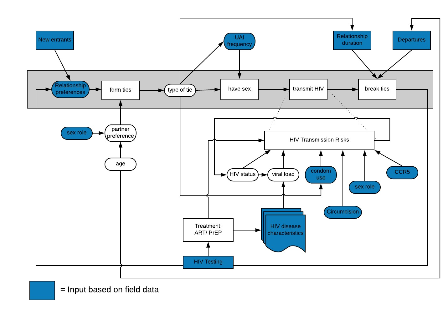
| Week number | Risk inflation factor EpiModel | Risk inflation factor NHS model | Risk Inflation NHS relative to EpiModel |
| 1 | 0.106 | 0.000 | 0.000 |
| 2 | 0.298 | 24.672 | 82.923 |
| 3 | 0.832 | 32.312 | 38.832 |
| 4 | 2.327 | 37.835 | 16.259 |
| 5 | 6.508 | 42.317 | 6.502 |
| 6 | 18.200 | 46.156 | 2.536 |
| 7 | 50.898 | 49.550 | 0.974 |
| 8 | 35.640 | 47.671 | 1.338 |
| 9 | 24.957 | 44.058 | 1.765 |
| 10 | 17.475 | 39.908 | 2.284 |
| 11 | 12.237 | 34.940 | 2.856 |
| 12 | 8.569 | 28.504 | 3.327 |
| 13 | 6.000 | 18.132 | 3.022 |
| Average onset stage (week 1-13) | 12.509 | ||
| 14 – 520 | 1.000 | 1.000 | 1.000 |
| 540 | 1.506 | 4.875 | 3.238 |
| 560 | 2.317 | 6.427 | 2.775 |
| 580 | 3.564 | 7.542 | 2.116 |
| 600 | 5.483 | 8.445 | 1.540 |
| 620 | 8.426 | 9.218 | 1.093 |
| Average AIDS stage (week 521-621) | 2.258 | ||
| Average throughout the infection (week 1 – 621) | 1.442 | ||
C: An example of the clarifying questions posed to the authors of the original model, and the consequent answers to these question.
Question 1: What happens to relationships in which one person turns 40 and leaves the model? More specifically, do all the relationships of this individual also get removed in the same step? Or does the younger partner stay in the relationship even though their older partner is no longer part of the simulation? The reason we ask is that in our model, ending the relationship severely reduces the duration of relationships for people in their early 30s and older (who are likely to be in relationships with people who are removed from the model.) Consequently, these people are more often exposed to new partners than they ought to be per the statistics in your supplemental material.
Answer 1: Relationships end when nodes leave the network. Because this introduces an artifact in the dissolution rate of partnerships, we adjust the dissolution coefficients to accommodate this exogenous force of edge removal. The adjustment, outlined at http://statnet.github.io/tut/NetUtils.html, has the effect of increasing the log odds coefficient (as the dissolution model is in reality simulating the process of relational persistence: 1 – dissolution).
Some related questions regarding population size and distribution:
Question 2a: First, regarding age distribution, we are unsure of what the age distribution is at the beginning of the simulation. Do you distribute the age evenly, or does everyone start at 18 like they do during the model’s runtime?
Answer 2a: Age is uniformly distributed across the possible ages in the modeled population: 18 to 40. See the code here that does that: https://github.com/statnet/EpiModelHIV/blob/master/R/estimation.R#L412.
Question 2b: Second, regarding the population size during runtime, we are not quite sure how your population stays stable around 10,000. In your Supplementary Technical Appendix (STA) you state, “All persons enter the network at age 18, which was the lower age boundary of our two main source studies. The number of new entries at each time step is based on a fixed rate (3 per 10,000 persons per weekly time step) that keeps the overall network size in a stable state over the time series of the simulations.”
If in 2a you distribute the age evenly across all 22 years at the beginning of the model (10,000 people / 1144 weeks), you get around 8 people per week. Consequently, around 8 people per time increment leave the simulation because they get too old, but only 3 new enter, for a net result of five fewer people in the simulation per week. As the population dwindles, even fewer people are added to the model because people are added as a function of the population size, further exacerbating the trend, resulting in a population of around 6770 after 10 years/520 time increments — and this is with neither HIV-related nor natural deaths in the model.
If in 2a everyone starts at 18, we get a larger population (typically around 11,680, again without deaths) but we have a population that is at most 28 years old after 10 years of runtime.
We feel quite sure that we’ve misunderstood something, but we’re not sure what. Would you please elaborate on how the population initiation and influx process works in more detail or clarify what we are misunderstanding?
Answer 2b: This was, unfortunately, an error in the Appendix. The actual per capita rate was 0.001 per week, which translates to 10 entries per week in a population of 10k. Also, we used a fixed product here (new entries = rate * starting population size) that does not account for any changes in population size over time because we did not conceptualize entries into the network as a birth process (MSM do not, as of yet, give birth to new MSM). See the code here for the rate definition (https://github.com/statnet/EpiModelHIV/blob/master/R/params.R#L275-L278) and application in the “birth” module (https://github.com/statnet/EpiModelHIV/blob/master/R/mod.births.R#L35-L38).
Question 3: What is the per-act HIV transmission probability factor for IEVs? On p. 19 in your STA your table with per-act HIV transmission probabilities shows the probabilities associated with respectively insertive and receptive acts, but does not mention IEV. Is it the same as receptive (since that is the highest risk), or is there are separate probability for IEVs?
Answer 3: IEV functions as a doubling of acts per “event” of AI, one insertive and one receptive. There was potential for transmission to occur in each independent act, with the transmission probability based on the directionality of each specific act. The code that does this is a little convoluted, but is all contained in the transmission module (https://github.com/statnet/EpiModelHIV/blob/master/R/mod.trans.R#L67-L72), where we set up the vector of transmission probabilities.
Question 4: On p5 of the STA, your research finds two different parameters that relate to the rate AI: race and sexual activity quintile of the individuals. But how are these two parameters related? Are they added or multiplied? Or something else? We suspect that we may be misunderstanding something about ART adherence, and its relationship to viral load.
Answer 4: First, although we have race built into the model, it is effectively ignored for this particular application by averaging over the race-specific parameters. In any case, the sexual activity quintile is a main effect, meaning that it is independent of the other variables in the network model. You can see that in the code here (https://github.com/statnet/PrEPGuidelines/blob/master/scripts/estimation/02.estim.R#L74-L78) where we set up the network models. The heterogeneity by activity quintile is governed by the nodefactor(“riskg”) term.
5a) Regarding ART adherence: On p. 17 of the STA your table shows the probabilities of people falling in and out of suppression with ART, but you also talk about cycling on and off treatment. In that table, what does it mean to fall out of, and re-achieve suppression? Does that mean that this person stops or starts using ART (i.e. cycling on and off treatment)? Or can a person be on ART, and still not be fully suppressed?
We initially interpreted it to mean that when e.g. white people become diagnosed, they have a \(\sim\).1 probability per week of going on treatment. Once they are in treatment, they have a 0.0071 probability of cycling off treatment per week and once they are off treatment, they have a 0.00291 probability of cycling back on every week. However, when we run this for a hypothetical population of 10,000 HIV+ people, we get the results in Figure 9.

Intuitively this makes sense to us, since for every individual, there is a high probability of going into treatment, then a low probability of falling out, but then an even lower probability of cycling back on – resulting in a population that mostly is not in treatment. In other words, we find it hard connect the individual per-week probabilities with the .614 for white black men and .651 for white men in the table on p 17. Are we misunderstanding what these numbers mean? Is this not what you mean by the per-week probabilities and “Proportion of those initiating ART who achieve full suppression?”
Answer 5a: For this issue, I recommend that you run the code yourself in R to see how things are functioning. As much as we tried to define everything precisely in the Appendix, it is only a partial (and as above, potentially incorrect at times) translation of the code. I’m not sure why you are seeing a decline in the proportion treated over time, while we see proportions on treatment and suppressed in equilibrium (at the 61% and 65% values in the table).
Question 5b: How is the effect of being on ART calculated? On the bottom of p 16 you say that there is a 3-month transition to the on-treatment viral loads, but we’re not sure how to interpret this vis a vis the question of falling in and out of suppression. If someone stays on ART for (at least) the 3-months, are they then not by definition fully suppressed? Again, we might be conflating ART and full suppression here if they are not the same thing, but we’re not sure how to interpret them on their own, and how they relate to each other.
Answer 5b: Take a look at the actual code in the viral load module (https://github.com/statnet/EpiModelHIV/blob/master/R/mod.vl.R). People have a suppression type assigned upon infection (partial vs full suppression), and they transition back and forth between set point viral load (4.5 log10) to either a partial suppression level (at 3.5 log10) or a full suppression level (at 1.5 log10). When they are on ART, VL declines based on a three-month slope to those nadirs, and when they are off ART, it increases back up to the set point.
Question 6: We are unsure of how to interpret some of the PrEP indications, specifically with regards to timing of the criteria. Your STA on p. 20 states indication 1 as, “UAI in a monogamous partnership with a partner not recently tested negative for HIV.” But how do these criteria relate to the time window? Does the relationship have to be monogamous at the time of the testing? Or does the relationship have to be monogamous at the time of the “qualifying” UAI? Or do they have to be monogamous throughout the entire window?
Answer 6: Throughout the entire window.
Consider this case: if two partners in a monogamous (by either of the two definitions) relationship have UAI, and then both partners find each a second partner (turning the relationship into a non-monogamous relationship by both definitions), and then one of them go in for testing – would that qualify for indication 1? Or vice versa – they are non-monogamous during a UAI, but then both end all their other relationships, and then one of them goes in for testing? Similarly for indications 2 and 3, how does the time window relate to the various cases in which people can shift in and out of eligibility?
If a man has UAI with a monogamous partner who recently (again within the past 6 months) also tests for HIV (the index man is by definition testing for HIV at the point of PrEP indication evaluation), then that index man is not indicated for PrEP based on condition 1. If the same man has UAI with more than two partners within any week, he is indicated for PrEP according to condition 2a. Indications for PrEP accumulate over the time risk window, such that any qualifying events during that period trigger an indication.
Relatedly, for indication 3, does the serodiscordant status of the relationship have to be known to either partner at the time of the AI? Again, consider a case: A couple that as far as they know are not serodiscordant have AI. One of them goes in for testing and is diagnosed as HIV+. The other person goes in, gets tested, and is HIV-. Would this person qualify? What if the AI happened outside of the window, but the HIV+ diagnosis of the partner happened during the window? The primary reason for these being important is that they change how permissive the indications are, and may even introduce non-monotonicity into the relationship between window-duration and permissiveness (.e. if they have to be monogamous throughout the entire window, at first a longer window will be more permissive, but then after a while it will be less permissive than a shorter window.)
In your example, the partner would need to get diagnosed, disclose to the index man (the man being evaluated for PrEP), and then have AI with him within the window. The diagnosis and disclosure may happen outside the window, but the AI needs to happen within the window.
D: The viral load progression when interacting with ART treatment.
Below we depict the viral-load levels as they were initially implemented across models, prior to alignment. In it these figures we show the effect of consuming one single dose of ART treatment (going in treatment one week and stop treatment the week after) at various times during the infection.
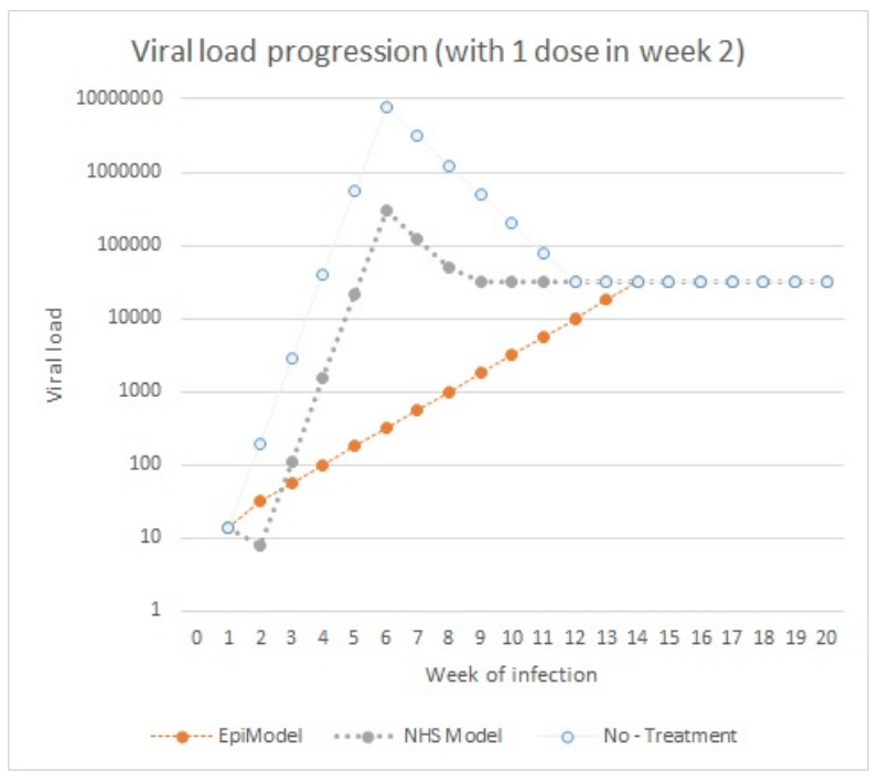


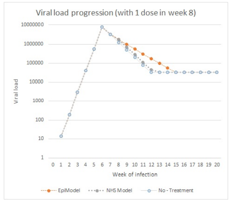
E: Viral load progression when interacting with ART treatment, after re-implementation according to the EpiModel conceptual model.
| No treatment | Single dose on day 2 | Single dose on day 4 | Single dose on day 6 | Single dose on day 8 | ||||||
| Week | EpiModel | NHS Model | EpiModel | NHS Model | EpiModel | NHS Model | EpiModel | NHS Model | EpiModel | NHS Model |
| 0 | 0.00 | 0.00 | 0.00 | 0.00 | 0.00 | 0.00 | 0.00 | 0.00 | 0.00 | 0.00 |
| 1 | 1.15 | 1.15 | 1.15 | 1.15 | 1.15 | 1.15 | 1.15 | 1.15 | 1.15 | 1.15 |
| 2 | 2.30 | 2.30 | 1.50 | 1.50 | 2.30 | 2.30 | 2.30 | 2.30 | 2.30 | 2.30 |
| 3 | 3.44 | 3.44 | 1.75 | 1.75 | 3.44 | 3.44 | 3.44 | 3.44 | 3.44 | 3.44 |
| 4 | 4.59 | 4.59 | 2.00 | 2.00 | 3.19 | 3.19 | 4.59 | 4.59 | 4.59 | 4.59 |
| 5 | 5.74 | 5.74 | 2.25 | 2.25 | 3.44 | 3.44 | 5.74 | 5.74 | 5.74 | 5.74 |
| 6 | 6.89 | 6.89 | 2.50 | 2.50 | 3.69 | 3.69 | 5.49 | 5.49 | 6.89 | 6.89 |
| 7 | 6.49 | 6.49 | 2.75 | 2.75 | 3.94 | 3.94 | 5.24 | 5.24 | 6.49 | 6.49 |
| 8 | 6.09 | 6.09 | 3.00 | 3.00 | 4.19 | 4.19 | 4.99 | 4.99 | 6.24 | 6.24 |
| 9 | 5.69 | 5.69 | 3.25 | 3.25 | 4.44 | 4.44 | 4.74 | 4.74 | 5.99 | 5.99 |
| 10 | 5.30 | 5.30 | 3.50 | 3.50 | 4.50 | 4.50 | 4.50 | 4.50 | 5.74 | 5.74 |
| 11 | 4.90 | 4.90 | 3.75 | 3.75 | 4.50 | 4.50 | 4.50 | 4.50 | 5.49 | 5.49 |
| 12 | 4.50 | 4.50 | 4.00 | 4.00 | 4.50 | 4.50 | 4.50 | 4.50 | 5.24 | 5.24 |
| 13 | 4.50 | 4.50 | 4.25 | 4.25 | 4.50 | 4.50 | 4.50 | 4.50 | 4.99 | 4.99 |
| 14 | 4.50 | 4.50 | 4.50 | 4.50 | 4.50 | 4.50 | 4.50 | 4.50 | 4.74 | 4.74 |
| 15 | 4.50 | 4.50 | 4.50 | 4.50 | 4.50 | 4.50 | 4.50 | 4.50 | 4.50 | 4.50 |
F: A description of the network formation process in the NHS model using pseudo code.
Prior to specifying the functioning of the network formation module we need to note 2 things:
- The aim of the network formation module is to form networks that are representative, this means that they follow the degree distribution taken from empirical data.
- Empirical data distinguishes three types of links, main, casual and one-time links. For the combination of main and casual there is a fixed distribution, whereas the degree in terms of one-time links is only conditional upon the main and casual links, see the tables below.
| 0 Casual ties | 1 Casual tie | 2 Casual ties | |
| 0 Main ties | 47.1 % | 16.7 % | 7.4 % |
| 1 Main tie | 22.0 % | 4.7 % | 2.1 % |
| 0 Casual ties | 1 Casual tie | 2 Casual ties | |
| 0 Main ties | 0.065 | 0.087 | 0.086 |
| 1 Main tie | 0.056 | 0.055 | 0.055 |
- Step 1: It is determined if there are enough individuals with main ties. If ties more ties are needed, step 2 is started, if not step 8 is started.
- Step 2: All individuals that are eligible to form a main tie are added to a list of main-tie-seekers
- Step 3: All individuals that are eligible to form a (additional) casual tie are added to a list of casual-tie-seekers
- Step 4: a) As long as there are more than two additional main ties needed (based on the above table)
- a. One of the main-tie-seekers is randomly chosen and selects another partner from the pool.
- b. Which individual is chosen is conditional upon:
- i. The alter not having a current tie to the agent
- ii. It being sexually compatible with the individual choosing
-
- iii. It being of the approximate age compared to the choosing individual
- c. A main tie is then formed among these partner
- b) As long as there are more than two additional casual ties needed (based on the above table)
- One of the casual-tie-seekers is randomly chosen and selects another partner from the pool.
- Which individual is chosen is conditional upon:
- The alter not having a current tie to the agent
- It being sexually compatible with the individual choosing
- It being of the approximate age compared to the choosing individual
- A casual tie is then formed among these partners
- Step 5: The list of main-tie-seekers is updated
- Step 6: The list of casual-tie-seekers is updated
- Step 7: go back to step 1
- Step 8: Conditional upon the number of main and casual ties each individual determines if he want a one-time tie this week.
- Step 9: all those seeking a one-time-tie are added to a list of one-time-tie-seekers
- Step 10: For as long as there are more than two individuals on the list of one-time-tie-seekers
- One of the one-time-tie-seekers is randomly chosen and selects a suitable partner. Again, which individual is chosen is conditional upon:
- The alter not having a current tie to the agent
- It being sexually compatible with the individual choosing
- It being of the approximate age compared to the choosing individual
- If not suitable partner can be found, the individual stop seeking a one-time-tie
- If a partner is found a one-time-tie is created among them, and both stop seeking a one-time-tie
Appendix G: Differences in the risks related to viral load, based on differing implementations of the risk calculation
After initially finding differences in the per act risks of transmission across implementations, we explored the behavior of both modules in greater detail. After substantial effort, we found the source of the misalignment to be the way risks calculations were implemented across the models. In EpiModel, log-odds were used in the risk calculations, whereas the NHS model, based on a reading of the technical appendix, used log-rates. While these are statistically indistinguishable at low levels of risks, they do differ when rates are moderate to high. In the process of aligning module behavior, we found that this variation had a significant effect on the per-act risks in scenarios with higher risks (e.g., in the acute stage) (see the figure below).

While the question of which implementation is more valid and/or desirable is scientifically relevant, we could not answer this question with the data at hand. What is more as our goal was alignment, we opted to adjust the NHS model implementation. By changing the implementation in the NHS model to log-odds, and strictly aligning the way in which risk calculations were executed across models, we found that the observed discrepancies disappeared and results of the per act risk were numerically identical (see Table 6 below). This observation is a yet another indication that small changes in the algorithm chosen and across implementations can have large implications for model alignment.
| NHS model used factors | NHS model used log-odds | |||||||
| HIV+ individual is recepetive | HIV+ individual is insertive | HIV+ individual is receptive | HIV+ individual is insertive | |||||
| Log of Viral load | Risk NHS | Risk EpiModel | Risk NHS | Risk EpiModel | Risk NHS | Risk EpiModel | Risk NHS | Risk EpiModel |
| 0 | 0.0004 | 0.0004 | 0.0010 | 0.0010 | 0.0004 | 0.0004 | 0.0010 | 0.0010 |
| 0.25 | 0.0004 | 0.0004 | 0.0012 | 0.0012 | 0.0004 | 0.0004 | 0.0012 | 0.0012 |
| 0.5 | 0.0006 | 0.0006 | 0.0015 | 0.0015 | 0.0006 | 0.0006 | 0.0015 | 0.0015 |
| 0.75 | 0.0007 | 0.0007 | 0.0019 | 0.0019 | 0.0007 | 0.0007 | 0.0019 | 0.0019 |
| 1 | 0.0009 | 0.0009 | 0.0023 | 0.0023 | 0.0009 | 0.0009 | 0.0023 | 0.0023 |
| 1.25 | 0.0011 | 0.0011 | 0.0029 | 0.0029 | 0.0011 | 0.0011 | 0.0029 | 0.0029 |
| 1.5 | 0.0014 | 0.0014 | 0.0036 | 0.0036 | 0.0014 | 0.0014 | 0.0036 | 0.0036 |
| 1.75 | 0.0017 | 0.0017 | 0.0046 | 0.0045 | 0.0017 | 0.0017 | 0.0045 | 0.0045 |
| 2 | 0.0022 | 0.0022 | 0.0057 | 0.0057 | 0.0022 | 0.0022 | 0.0057 | 0.0057 |
| 2.25 | 0.0027 | 0.0027 | 0.0071 | 0.0071 | 0.0027 | 0.0027 | 0.0071 | 0.0071 |
| 2.5 | 0.0034 | 0.0034 | 0.0089 | 0.0089 | 0.0034 | 0.0034 | 0.0089 | 0.0089 |
| 2.75 | 0.0042 | 0.0042 | 0.0112 | 0.0111 | 0.0042 | 0.0042 | 0.0111 | 0.0111 |
| 3 | 0.0053 | 0.0053 | 0.0140 | 0.0138 | 0.0053 | 0.0053 | 0.0138 | 0.0138 |
| 3.25 | 0.0066 | 0.0066 | 0.0175 | 0.0172 | 0.0066 | 0.0066 | 0.0172 | 0.0172 |
| 3.5 | 0.0083 | 0.0082 | 0.0219 | 0.0215 | 0.0082 | 0.0082 | 0.0215 | 0.0215 |
| 3.75 | 0.0104 | 0.0103 | 0.0274 | 0.0268 | 0.0103 | 0.0103 | 0.0268 | 0.0268 |
| 4 | 0.0130 | 0.0128 | 0.0343 | 0.0333 | 0.0128 | 0.0128 | 0.0333 | 0.0333 |
| 4.25 | 0.0162 | 0.0160 | 0.0429 | 0.0414 | 0.0160 | 0.0160 | 0.0414 | 0.0414 |
| 4.5 | 0.0203 | 0.0199 | 0.0536 | 0.0513 | 0.0199 | 0.0199 | 0.0513 | 0.0513 |
| 4.75 | 0.0254 | 0.0248 | 0.0671 | 0.0635 | 0.0248 | 0.0248 | 0.0635 | 0.0635 |
| 5 | 0.0317 | 0.0309 | 0.0839 | 0.0785 | 0.0309 | 0.0309 | 0.0785 | 0.0785 |
| 5.25 | 0.0397 | 0.0384 | 0.1050 | 0.0966 | 0.0384 | 0.0384 | 0.0966 | 0.0966 |
| 5.5 | 0.0497 | 0.0477 | 0.1314 | 0.1184 | 0.0477 | 0.0477 | 0.1184 | 0.1184 |
| 5.75 | 0.0621 | 0.0591 | 0.1644 | 0.1446 | 0.0591 | 0.0591 | 0.1446 | 0.1446 |
| 6 | 0.0777 | 0.0730 | 0.2057 | 0.1756 | 0.0730 | 0.0730 | 0.1756 | 0.1756 |
| 6.25 | 0.0973 | 0.0900 | 0.2573 | 0.2119 | 0.0900 | 0.0900 | 0.2119 | 0.2119 |
| 6.5 | 0.1217 | 0.1105 | 0.3219 | 0.2538 | 0.1105 | 0.1105 | 0.2538 | 0.2538 |
| 6.75 | 0.1523 | 0.1351 | 0.4027 | 0.3015 | 0.1351 | 0.1351 | 0.3015 | 0.3015 |
| 7 | 0.1905 | 0.1644 | 0.5039 | 0.3549 | 0.1644 | 0.1644 | 0.3549 | 0.3549 |
Appendix H: Alignment of the number of sex acts across implementations

This figure clearly shows how without incorporating the scalar for the number of sex acts, the number of sex acts across implementations vastly differed, after adding this scalar to the NHS model the distribution of sex act was is distributionally aligned.
I: The one-tick-test, testing for significant differences under the poison assumption for world states.
Based on the observation that the incidence of a given repetition of the one-tick-test is drawn from a Poisson distribution we can devise a formal test to see if the result from both implementations are in fact drawn from a distribution with the same mean value. This test combines the observations of both implementations, but keep track of the source of the observation by means of a dummy variable. Next it is tested if the dummy variable is a significant predictor of the mean of the Poisson distribution. If a significant effect is found for the dummy variable this is an indication that the source of data matters, and that there is a difference across implementation. An insignificant result indicates that there are no differences across implementations. For each network we can conduct this test, resulting in a total of 50 observations.
The results of the initial test for alignment are presented below. The first figure shows the significance levels that were obtained from the test across the 50 networks. It reveals that 10 out of the 50 tests yielded significant results at the 0.05 confidence level, which is much more than expected. The second figure shows the coefficients for the test across the 50 networks, and reveal that the average coefficient is slightly above 0, indicating that the NHS has slightly higher mean in the Poisson distribution.


References
ARIFIN, N. S. M., Davis, G. J., & Zhou, Y. (2010, July). Verification & validation by docking: a case study of agent-based models of Anopheles gambiae. In Proceedings of the 2010 Summer Computer Simulation Conference (pp. 236-243). Society for Computer Simulation International.
AXTELL, R., Axelrod, R., Epstein, J. M., & Cohen, M. D. (1996). Aligning simulation models: A case study and results. Computational & Mathematical Organization Theory, 1(2), 123-141. [doi:10.1007/bf01299065]
AXTELL, R., Epstein, J.M., Dean, J.S., Gumerman, G.J., Swedlund, A.C., Harburger, J., Chakravarty, S., Hammond, R., Parker, J., Parker, M. (2002). Population growth and collapse in a multiagent model of the Kayenta Anasazi in Long House Valley. Proceedings of the National Academy of Sciences, 99, suppl 3, 7275–7279. [doi:10.1073/pnas.092080799]
BHAVNANI, R. (2003). Adaptive Agents, Political Institutions and Civic Traditions in Modern Italy. Journal of Artificial Societies and Social Simulation, 6(4), 1: https://www.jasss.org/6/4/1.html.
BONABEAU, E. (2002). Agent-based modeling: Methods and techniques for simulating human systems. Proceedings of the National Academy of Sciences, 99-3, 7280-7287. [doi:10.1073/pnas.082080899]
CDC. (2014). Preexposure Prophylaxis for the Prevention of HIV Infection in the United States–2014: A Clinical Practice Guideline.
CHAMBERS, J. M. (2018). Graphical Methods for Data Analysis. London: CRC Press.
COHEN, M. S., Chen, Y. Q., McCauley, M., Gamble, T., Hosseinipour, M. C., Kumarasamy, N., . . . Fleming, T. R. (2011). Prevention of HIV-1 Infection with Early Antiretroviral Therapy. New England Journal of Medicine , 365(6), 493-505.
COLLINS, A., Petty, M., Vernon-Bido, D., & Sherfey, S. (2015). A Call to Arms: Standards for Agent-Based Modeling and Simulation. Journal of Artificial Societies and Social Simulation, 18(3), 12: https://www.jasss.org/18/3/12.html [doi:10.18564/jasss.2838]
DONKIN, E., Dennis, P., Ustalakov, A., Warren, J., & Clare, A. (2017). Replicating complex agent based models, a formidable task. Environmental Modelling & Software, 92, 142-151. [doi:10.1016/j.envsoft.2017.01.020]
EDMONDS, B., & Hales, D. (2003). Replication, Replication and Replication: Some Hard Lessons from Model Alignment. Journal of Artificial Societies and Social Simulation, 6(4), 11: https://www.jasss.org/6/4/11.html.
EPSTEIN, J. M. (1998). Zones of cooperation in demographic prisoner's dilemma. Complexity, 4(2), 36-48.
EPSTEIN, J. M. (2009). Modelling to contain pandemics. Nature, 460, 687. [doi:10.1038/460687a]
FACHADA, N., & Rosa, A. C. (2017, May). Assessing the feasibility of OpenCL CPU implementations for agent-based simulations. In Proceedings of the 5th International Workshop on OpenCL (p. 4). ACM. [doi:10.1145/3078155.3078174]
GOODREAU, S. M., Carnegie, N. B., Vittinghoff, E., Lama, J. R., Fuchs, J. D., Sanchez, J., & Buchbinder, S. P. (2014). Can Male Circumcision Have an Impact on the HIV Epidemic in Men Who Have Sex with Men? PLoS ONE, 9(7). [doi:10.1371/journal.pone.0102960]
GOODREAU, S. M., Carnegie, N. B., Vittinghoff, E., Lama, J. R., Sanchez, J., Grinsztejn, B., . . . Sullivan, P. S. (2012). What Drives the US and Peruvian HIV Epidemics in Men Who Have Sex with Men (MSM)? PLoS ONE, 7(11). [doi:10.1371/journal.pone.0050522]
GUNARATNE and Garibay (2017) Alternate social theory discovery using genetic programming: towards better understanding the artificial Anasazi, GECCO '17 Proceedings of the Genetic and Evolutionary Computation Conference [doi:10.1145/3071178.3071332]
GRIMM, V., Augusiak, J., Focks, A., Frank, B. M., Gabsi, F., Johnston, A. S. A., . . . Railsback, S. F. (2014). Towards better modelling and decision support: Documenting model development, testing, and analysis using TRACE. Ecological Modelling, 280, 129-139. [doi:10.1016/j.ecolmodel.2014.01.018]
GRIMM, V., Berger, U., Bastiansen, F., Eliassen, S., Ginot, V., Giske, J., . . . DeAngelis, D. L. (2006). A standard protocol for describing individual-based and agent-based models. Ecological Modelling, 198(1), 115-126. [doi:10.1016/j.ecolmodel.2006.04.023]
GRIMM, V., Berger, U., DeAngelis, D. L., Polhill, J. G., Giske, J., & Railsback, S. F. (2010). The ODD protocol: A review and first update. Ecological Modelling, 221(23), 2760-2768. [doi:10.1016/j.ecolmodel.2010.08.019]
GRIMM, V., Polhill, G., & Touza, J. (2017). Documenting Social Simulation Models: The ODD Protocol as a Standard. In B. Edmonds & R. Meyer (Eds.), Simulating Social Complexity: A Handbook (pp. 349-365). Cham: Springer International Publishing. [doi:10.1007/978-3-319-66948-9_15]
GRIMM, V., Revilla, E., Berger, U., Jeltsch, F., Mooij, W. M., Railsback, S. F., . . . DeAngelis, D. L. (2005). Pattern-Oriented Modeling of Agent-Based Complex Systems: Lessons from Ecology. Science, 310(5750), 987-991. [doi:10.1126/science.1116681]
HAYES, I. J. (1986). Specification directed module testing. IEEE Transactions on Software Engineering, SE-12(1), 124-133. [doi:10.1109/tse.1986.6312926]
HERNÁNDEZ-ROMIEU, A. C., Sullivan, P. S., Rothenberg, R., Grey, J., Luisi, N., Kelley, C. F., & Rosenberg, E. S. (2015). Heterogeneity of HIV Prevalence Among the Sexual Networks of Black and White Men Who Have Sex with Men in Atlanta: Illuminating a Mechanism for Increased HIV Risk for Young Black Men Who Have Sex with Men. Sexually Transmitted Diseases, 42(9), 505-512. [doi:10.1097/olq.0000000000000332]
HJORTH, A., Vermeer, W., Wilensky, U. (2020). “The NetLogo HIV Spread Model Exploring Impact of PrEP Indication Guidelines” (Version 1.0.0). CoMSES Computational Model Library. Retrieved from: https://www.comses.net/codebases/d3d45a7e-24a4-42e9-a44b-e6e8e293e578/releases/1.0.0/.
HUGHES, J. P., Lingappa, J. R., Celum, C., Baeten, J. M., Wald, A., Farquhar, C., . . . Kilembe, W. (2012). Determinants of Per-Coital-Act HIV-1 Infectivity Among African HIV-1-Serodiscordant Couples. The Journal of Infectious Diseases , 205(3), 358-365. [doi:10.1093/infdis/jir747]
JANSSEN, M. A. (2009). Understanding artificial anasazi. Journal of Artificial Societies and Social Simulation 12(4), 13: https://www.jasss.org/12/4/13.html
JENNESS, S. M., Goodreau, S. M., & Morris, M. (2018). EpiModel: An R Package for Mathematical Modeling of Infectious Disease over Networks. Journal of Statistical Software, 84, 8. [doi:10.18637/jss.v084.i08]
JENNESS, S. M., Goodreau, S. M., Rosenberg, E., Beylerian, E. N., Hoover, K. W., Smith, D. K., & Sullivan, P. (2016). Impact of the Centers for Disease Control's HIV Preexposure Prophylaxis Guidelines for Men Who Have Sex with Men in the United States. The Journal of Infectious Diseases, 214(12), 1800-1807. [doi:10.1093/infdis/jiw223]
KOLLMAN, K., Miller, J. H., & Page, S. E. (1997). Political Institutions and Sorting in a Tiebout Model. The American Economic Review, 87(5), 977-992.
KRIVITSKY, P. N., & Handcock, M. S. (2014). A separable model for dynamic networks. Journal of the Royal Statistical Society: Series B (Statistical Methodology), 76(1), 29-46. [doi:10.1111/rssb.12014]
LITTLE, S. J., McLean, A. R., Spina, C. A., Richman, D. D., & Havlir, D. V. (1999). Viral Dynamics of Acute HIV-1 Infection. The Journal of Experimental Medicine, 190(6), 841-850. [doi:10.1084/jem.190.6.841]
LIU, A. Y., COHEN, S. E., VITTINGHOFF, E., ANDERSON, P. L., DOBLECKI-LEWIS, S., BACON, O., . . . KOLBER, M. A. (2016). Preexposure Prophylaxis for HIV Infection Integrated with Municipal- and Community-Based Sexual Health Services. JAMA Internal Medicine, 176(1), 75-84. [doi:10.1001/jamainternmed.2015.4683]
LORENZ, E. (1972). Predictability: does the flap of a butterfly's wings in Brazil set off a tornado in Texas? Resonance, 20(03).
MACY, M. W., & Sato, Y. (2002). Trust, cooperation, and market formation in the U.S. and Japan. PNAS 99(3), 7214-7220. [doi:10.1073/pnas.082097399]
MAGLIO, P. P., Sepulveda, M.-J., & Mabry, P. L. (2014). Mainstreaming Modeling and Simulation to Accelerate Public Health Innovation. American Journal of Public Health , 104(7), 1181-1186. [doi:10.2105/ajph.2014.301873]
MARMOR, M., Sheppard, H. W., Donnell, D., Bozeman, S., & Celum, C. (2001). Homozygous and HeterozygousCCR5-Δ32Genotypes Are Associated With Resistance to HIV Infection. JAIDS Journal of Acquired Immune Deficiency Syndromes, 27(5), 472-481. [doi:10.1097/00126334-200108150-00009]
MERLONE, U., Sonnessa, M., & Terna, P. (2008). Horizontal and Vertical Multiple Implementations in a Model of Industrial Districts. Journal of Artificial Societies and Social Simulation, 11(2), 5: https://www.jasss.org/11/2/5.html.
MIODOWNIKA, D., Cartriteb, B., & Bhavnani, R. (2010). Between Replication and Docking: "Adaptive Agents, Political Institutions, and Civic Traditions" Revisited. Journal of Artificial Societies and Social Simulation, 13(3), 1: https://www.jasss.org/13/3/1.html. [doi:10.18564/jasss.1627]
MUGAVERO, M. J., Amico, K. R., Horn, T., & Thompson, M. A. (2013). The State of Engagement in HIV Care in the United States: From Cascade to Continuum to Control. Clinical Infectious Diseases, 57(8), 1164-1171. [doi:10.1093/cid/cit420]
NEWMAN, M. E. J. (2003). The Structure and Function of Complex Networks. SIAM review, 45(2), 167-256.
POTTING, R. P. J., Perry, J. N., & Powell, W. (2005). Insect behavioural ecology and other factors affecting the control efficacy of agro-ecosystem diversification strategies. Ecological Modelling, 182(2), 199-216. [doi:10.1016/j.ecolmodel.2004.07.017]
RADAX, W., & Rengs, B. (2010). Prospects and Pitfalls of Statistical Testing. Insights from Replicating the demographic prisoners Dilemma. Journal of Artificial Societies and Social Simulation, 13(4), 1: https://www.jasss.org/13/4/1.html [doi:10.18564/jasss.1634]
RAND, W. & Rust, R.T. (2011) Agent-based modeling in marketing: Guidelines for rigor, International Journal of Research in Marketing, 28(3), 181–193. [doi:10.1016/j.ijresmar.2011.04.002]
SEAGREN, C. W. (2015). A Replication and Analysis of Tiebout Competition Using an Agent-Based Computational Model. Social Science Computer Review, 33(2), 198-216. [doi:10.1177/0894439314534810]
STONEDAHL, F. & Wilensky, U. (2010). Finding forms of flocking: Evolutionary search in ABM parameter-spaces. International Workshop on Multi-Agent Systems and Agent-Based Simulation. Springer, 61–75. [doi:10.1007/978-3-642-18345-4_5]
SULLIVAN, P. S., Rosenberg, E. S., Sanchez, T. H., Kelley, C. F., Luisi, N., Cooper, H. L., . . . Peterson, J. L. (2015). Explaining racial disparities in HIV incidence in black and white men who have sex with men in Atlanta, GA: a prospective observational cohort study. Annals of Epidemiology, 25(6), 445-454. [doi:10.1016/j.annepidem.2015.03.006]
THIELE, J. C., & Grimm, V. (2015). Replicating and breaking models: good for you and good for ecology. Oikos, 124(6), 691-696. [doi:10.1111/oik.02170]
VERMEER, W., Koppius, O., & Vervest, P. (2018). The Radiation-Transmission-Reception (RTR) model of propagation: Implications for the effectiveness of network interventions. PLoS ONE, 13(12). [doi:10.1371/journal.pone.0207865]
WELLER, S. C., & Davis‐Beaty, K. (2002). Condom effectiveness in reducing heterosexual HIV transmission. Cochrane Database of Systematic Reviews(1). [doi:10.1002/14651858.cd003255]
WILENSKY, U. (1999). NetLogo. http://ccl.northwestern.edu/netlogo/. Center for Connected Learning and Computer-Based Modeling.
WILENSKY, U., & Rand, W. (2007). Making Models Match: Replicating an Agent-Based Model. Journal of Artificial Societies and Social Simulation, 10(4), 2: https://www.jasss.org/10/4/2.html.
WILENSKY, U., & Rand, W. (2015). An introduction to Agent-Based Modeling: Modeling Natural, Social, and Engineered Complex Systems with NetLogo. Cambridge, MA: MIT Press.
WILL, O., & Hegselmann, R. (2008). A Replication that Failed? on the Computational Model in 'Michael W. Macy and Yoshimichi Sato: Trust, Cooperation and Market Formation in the U.S. and Japan. Proceedings of the National Academy of Sciences, May 2002'.Journal of Artificial Societies and Social Simulation , 11(3), 3: https://www.jasss.org/11/3/3.html.
WIYSONGE, C. S., Kongnyuy, E. J., Shey, M., Muula, A. S., Navti, O. B., Akl, E. A., & Lo, Y. R. (2011). Male circumcision for prevention of homosexual acquisition of HIV in men. Cochrane Database of Systematic Reviews(6). [doi:10.1002/14651858.cd007496.pub2]
ZIMMERMAN, P. A., Buckler-White, A., Alkhatib, G., Spalding, T., Kubofcik, J., Combadiere, C., . . . Murphy, P. M. (1997). Inherited Resistance to HIV-1 Conferred by an Inactivating Mutation in CC Chemokine Receptor 5: Studies in Populations with Contrasting Clinical Phenotypes, Defined Racial Background, and Quantified Risk. Molecular Medicine, 3(1), 23-36. [doi:10.1007/bf03401665]