
Introduction
CommunityRx (CRx), developed with the support of a Health Care Innovation Award from the U.S. Center for Medicare and Medicaid Innovation (CMMI), is an information-based health intervention designed to improve population health by systematically connecting people to a broad range of community-based resources for health-maintenance, wellness, disease management and care-giving (Lindau et al. 2016, 2019). The CRx program was initially implemented on Chicago’s South Side and covered 16 ZIP codes, encompassing an area of 106 square miles with a population of 1.08M people. Two studies were conducted between 2012-2016, a large observational study and a pragmatic clinical trial, to evaluate the impact of the CRx intervention on health, healthcare utilization, and self-efficacy.
The CRx intervention is centered around the “HealtheRx” (or HRx), a 3-page printed list of community resources personalized to a patient’s characteristics, location, and diagnoses (Lindau et al. 2016). Community resources prescribed in the HRx include resources to address basic needs (e.g., food and housing), physical and mental wellness (e.g., fitness, counseling), disease management (e.g., smoking cessation, weight loss), and care-giving (e.g., respite care for a person with dementia.) The goal of the information intervention via the HRx is to effect an increase in utilization in community resources and, ultimately, health. The HRx represented the primary vector of information diffusion regarding community resources, while the diffusion of this information into the patient’s social and interaction networks represented the secondary diffusion vectors.
An information-based intervention like CRx spreads non-linearly across the population via the individuals’ networks, to other people who did not initially receive the intervention and, in turn, can impact their behaviors by affecting their decision-making related to utilizing community resources. Accurate assessment of such multi-level interventions necessitates moving beyond traditional methods like prospective trials (Kaligotla et al. 2018; Lindau et al. 2016). A computational agent-based model (ABM) was thus developed to investigate the impact of the CRx intervention. The development of the CRx ABM was informed by empirical data from the CRx studies and other observational, experimental, and expert informant sources (Kaligotla et al. 2018). This paper describes the characterization of parameter space of the CRx ABM through an implementation of an Active Learning (AL) (Settles 2012) model exploration (ME) algorithm at high-performance computing (HPC) scales using the EMEWS framework (Ozik et al. 2016), as a step towards model validation.
Building valid computational models at scale
Our broad research goal is to integrate clinical trial methodology with agent-based modeling, to enable in silico experimentation at scale, to inform clinical trial design and evaluation, and to amplify thereby the impact of individual-level clinical trials of information-based population health interventions. A challenge in using ABMs to analyze interventions or run computational experiments is in the validation that these computational models adequately represent the dynamics of interest. Building validated models requires a robust characterization of model parameter spaces to facilitate the calibration of model outputs against empirical observations.
The characterization of parameter spaces, however, is often difficult to achieve in practice for complex, expensive-to-run models with large parameter spaces. Sufficient characterization of high-dimensional parameter spaces is usually infeasible using brute force techniques that attempt to span the space with an a priori defined set of points. Instead, adaptive, or sequential, heuristic techniques can be used: techniques that strategically sample larger parameter spaces by selectively applying computational budgets to more important regions, e.g., History Matching (Holden et al. 2018; Williamson et al. 2013), Gaussian process surrogate models (Baker et al. 2020; Kennedy & O’Hagan 2001), and stochastic equilibrium models (Flötteröd et al. 2011). These sequential model exploration techniques, however, are difficult to implement in a generalizable way and at scale. The computational complexity involved in building validated models (in terms of effort and computational power) impedes the broader applicability of ABMs and simulation models in general.
In this paper, we describe our progress towards building a validated CRx ABM through large-scale model exploration techniques. We describe a random forest meta-model to iteratively classify and characterize the input parameter space into potentially viable and non-viable regions with respect to observed empirical data, as the initial step in validating our model. This stepwise tightening approach is similar to history matching (Holden et al. 2018) and is driven by the goal of reducing computational costs associated with the analysis of complex models. We also describe the parallelization techniques and frameworks that enable our model exploration approach on HPC resources. The rest of the paper is organized as follows: Section 2 describes the development and implementation of the CRx ABM. Section 3 introduces the AL workflow we implement to calibrate the CRx ABM against empirical observations. Section 4 describes parallelization techniques that enable model performance gains needed for efficient model exploration, followed by a description of the HPC AL workflow implemented with the EMEWS framework. Section 5 demonstrates how the AL algorithm characterizes the large CRx ABM parameter space. We conclude and highlight future research in Section 6.
CRx ABM and Implementation
This section provides an overview of the CRx ABM and its implementation. We created a synthetic environment with statistical equivalence to the geographical region that corresponds to the CRx study area, on which we model the diffusion of information and its effect on agent decision behavior. A detailed description of the model is available in Kaligotla et al. (2018).
Synthetic population
The synthetic environment in the CRx model consists of 3 entities - a population of agents (\(\mathbf{P}\)), resources (\(\mathbf{R}\)), and clinics (\(\mathbf{C}\)). Using SPEW (Synthetic Population and Ecosystems of the World) data from (Gallagher et al. 2018), we create a population of 802,191 agents with static sociodemographic characteristics matching the population of the South and West sides of Chicago (ages 16 and older since the HRx information sheet for patients younger than 16 was typically given to an accompanying adult), each of whom are assigned to a household, and work or school location. Additionally, using CRx and MAPSCorps data from www.mapscorps.org (Makelarski et al. 2013), we build a synthetic physical environment in which agents move, consisting of 4,903 unique places that provide services, including health-related services. The set of places also includes health care clinics where an agent could receive a HRx and exchange information with other agents about community resources.
Agents perform an activity during each 1-hour time-step of a 24-hour activity schedule. Agents are randomly assigned an activity schedule each simulated day based on their sociodemographic characteristics. The activity schedules of the agents were developed using the American Time Use Survey (ATUS) dataset (https://www.bls.gov/tus/data.htm). Activities are mapped onto relevant services that are associated with geo-located resources in (\(\mathbf{R}\)). This approach allows us to connect two separate data sets, SPEW and ATUS, and maintain a stochastic variability of the population activities and use of resources based on matching demographic characteristics.
Agent decision behavior
We model an agent’s health maintenance behavior through an agent-based decision model. Agents can encounter two general types of activities in their activity schedules. The first type of activities are related to health maintenance behaviors, which correspond to types of services that are frequently referred to by HRxs. These activities provide a choice in behavior - either to decide in favor of engaging in a health maintenance related activity (use of wellness or health promoting community resource) in question, denoted by Decision A, or not, denoted by Decision B. The second type of agent activities does not contain any decision-making component. The agent will simply do the activity in question at the specified time if a relevant service type is known to the agent.
We model the use of a resource \(j \in \mathbf{R}\), by agent \(i \in \mathbf{P}\), at time \(t\in {0,1,2,\dots,T}\) as a decision model whose functional form is given by:
| $$\begin{cases} \textit{Decision A} & \text{If}\ \frac{\beta_{i,j}^t}{(\gamma_j \times \delta^t_{i,j})} > \alpha_i \\ \textit{Decision B} & \text{otherwise} \end{cases}: \ \alpha, \beta, \gamma , \delta \in (0,1)$$ | (1) |
Here \(\alpha_i\), the agent activation score, denotes an individual agent’s intrinsic threshold for health maintenance activities, resource score \(\beta_{i,j}^t\) denotes an agent’s dynamic level of knowledge of the particular resource and its associated benefits, \(\gamma_j\) is a measure of resource inertia, the inherent difficulty associated with performing an activity at a resource, and \(\delta_{i,j}^t\) represents the distance threshold between an individual agent and the location for a resource/activity. An agent thus chooses to perform a health related activity, Decision A, only when their activation threshold \(\alpha_i\) is exceeded by a function of their perceived characteristics of resource \(j\) at time \(t\).
Agent activation score values (\(\alpha_i\) ) are derived from Table 1 in (Skolasky et al. 2011), stochastically matched to individual agents via demographic characteristics. An agent with a high activation score implies a higher level of difficulty in performing tasks, and ceteris paribus, is therefore less likely to perform health related activities. The resource score ( \(\beta_{i,j}^t\)) is dynamic (explained in the following subsection) and evolves over time based on “dosing,” a term we use in this paper to refer to an agent’s exposure to information about a particular resource at a specific time. The higher the resource score, the higher the likelihood of an agent performing an activity. Delta (\(\delta_{i,j}^t\)) accounts for a "location effect" with respect to an agent’s decision – the higher the distance to an activity, the lower the likelihood of an agent performing an activity. We derive resource-specific thresholds for what we classify as low-medium-high resource distances using survey data from Garibay et al.(2014).
Information diffusion
We model the dynamic diffusion of information as a function of agent interactions, the source of information dosing, and the evolution of an agent’s knowledge with respect to the information. Agents following their activity schedules will find themselves geographically co-located with other agents. All co-located agents interact and exchange information about resources with some probability. We model this probabilistic information exchange as dependent on an agent’s propensity to share information, and the amenability of the activity itself to information sharing, e.g., the propensity to share information while an agent’s activity is “socializing and communicating with others" will be higher than an activity like”doing aerobics." We associate a scaled propensity score for different types of activities representing the different likelihoods of an agent sharing information with other agents who are co-located at that time – none (e.g., sleeping), low (e.g., doing aerobics), medium (e.g., grocery shopping), and high (e.g., socializing and communicating with others). The propensity scores and their mapping to the activity types were obtained from expert surveys.
Different sources for information dosing are considered in our model (to account for the relative trustworthiness of the source of information) and are denoted by a set \(X\in \{\text{Doctor, Nurse, PSR, Use, Peer}\}\). \(\epsilon_{x} \in (0,1), x\in X\) is a dosing parameter representing the effect of each dosing source’s relative trustworthiness on an agent’s \(\beta\). \(n_{ij}^{t}=1\) denotes the instance of information dosing for agent \(i\) about resource \(j\), at time \(t\) by some source \(x\in X\). An agent’s evolving level of knowledge for a particular resource and its associated benefits is described through the time evolution of \(\beta_{i,j}^t\), given by Equation 2, where \(\lambda\) is a decay parameter over time, representing the effect of a resource receding from an agent’s attention, possibly replaced with knowledge about other resources, and \(\epsilon_{x} \in (0,1)\), the dosing parameter for the dosing source’s effect on recall, and \(n_{ij}^{t}=1\) denotes the instance of information dosing for agent \(i\) about resource \(j\), at time \(t\) by a dosing source \(X\).
| $$\forall i, \forall j, \ \beta_{i,j}^{0} =f_{\beta}(I), \ \beta_{i,j}^{t} = \begin{cases} \lambda\times\left(\beta_{i,j}^{t-1}\right)^{\epsilon_{x} (1-\beta_{i,j}^{t-1}) + \beta_{i,j}^{t-1}} & \text{If} \ n_{ij}^{t}=1 \\ \lambda\times\left(\beta_{i,j}^{t-1}\right) & \text{otherwise} \end{cases} : \lambda \in (0,1) , x\in \{1,2,\dots,5\} $$ | (2) |
Initialization of \(\beta\) follows from a function \(f_{\beta}(I)\), which considers the implicit assumption that an agent (at time 0) knows between 10 and 100 resources in a near (1-mile radius) distance around their home location, and 1 to 5 resources each in the medium (less than 3 miles) and far (more than 3 miles) distances. Each of these initial known resources has a \(\beta\) score equal to \(\kappa\), while all other resources are unknown to the agent, hence having an effective \(\beta\) score of 0. The CRx intervention was modeled by replicating the original algorithms that generated an HRx based on patient demographics, home address, health and social conditions, and preferred language (Kaligotla et al. 2018).
CRx model implementation
The CRx model is implemented in C++ using the Repast for High Performance Computing (Repast HPC) (Collier & North 2013) and the Chicago Social Interaction Model (chiSIM) (Macal et al. 2018) toolkits. Repast HPC is a C++-based agent-based model framework for implementing distributed ABMs using MPI (Message Passing Interface). chiSIM, built on Repast HPC, is a framework for implementing models that simulate the mixing of a synthetic population. chiSIM itself is a generalization of a model of community associated methicillin-resistant Staphylococcus aureus (CA-MRSA) (Macal et al. 2014). In the chiSIM-based CRx model, each agent in the simulated population resides in a place (a household). Places are created on a process and remain there. Agents move among the processes according to their activity profiles. When an agent selects a next place to move to, the agent may stay on its current process, or it may have to move to another process if its next place is not on the agent’s current process. A load-balancing algorithm is applied to the synthetic population to create an efficient distribution of agents and places, minimizing this computationally expensive cross-process movement of agents and balancing the number of agents on each process (Collier et al. 2015). The CRx model and the workflow code used to implement the parameter space characterization experiments are publicly available (at the following URL: https://github.com/jozik/community-rx).
Model Exploration using Active Learning
Model calibration refers to the process of fitting simulation model output to observed empirical data by identifying values for the set of calibration parameters (Kennedy & O’Hagan 2001). We note that we use the term model exploration to refer to the family of approaches used for characterizing model parameter spaces, including model calibration.
Model calibration techniques described in the extant literature generally fall into two approaches: direct calibration methods and model-based methods (Xu 2017). Direct calibration methods generally utilize direct search methods, e.g., stochastic approximation (Yuan et al. 2012) or discrete optimization (Xu et al. 2014), to explore the parameter space and identify calibration values that minimize differences between model outputs and empirical observations. Model-based methods, including Bayesian calibration methods, make use of surrogate models, e.g., Gaussian process (Kennedy & O’Hagan 2001) or stochastic equilibrium models (Flötteröd et al. 2011), to combine empirical observations with prior knowledge, and to obtain a posterior distribution on a model’s calibration parameters. Xu (2017) provides an overview of the merits and limitations of each of these approaches. Baker et al. ( 2020) provides a comprehensive review of Gaussian process surrogate models used for calibrating stochastic simulators. The method described in this paper falls into sequential model-based approaches.
The increasing availability of computational resources has emboldened advances in the exploration and calibration of simulation models using new approaches. Han et al. (2009), for instance, introduce a statistical methodology for simultaneously determining empirically observable and unobservable parameters in settings where data are available. Reuillon et al.( 2015) also describes an automated calibration process, computing the effect of each calibration parameter on overall agent-based model behavior, independently from others. Particularly relevant to large scale parameter space exploration, Lamperti et al. (2018) describes a combination of machine learning and adaptive sampling to build a surrogate meta-model that combines model simulation with output analysis to calibrate their ABM. Another multi-method example of large-scale parameter space exploration is the use of dimension reduction techniques, common in climate science. (Higdon et al. 2008), for instance, describe the combination of dimension reduction techniques and regression models to enable computation at scale. Also common in this class of model calibration is the use of history matching as an alternative to probabilistic matching (Williamson et al. 2013). Like traditional calibration, history matching identifies regions of parameter space that result in acceptable matches between simulation output and empirically observed data. This method has been used to calibrate complex simulators across domains - oil reservoir modeling (Craig et al. 1997), epidemiology (Andrianakis et al. 2015), and climate modeling (Edwards et al. 2011; Holden et al. 2018)
Our primary goal in this paper is to characterize the parameter space of the CRx ABM, i.e., identify parameter value combinations where model output is potentially compatible with empirical data. The model exploration techniques described in this section partition the parameter space into potentially viable and non-viable regions. This approach has the benefit of allowing subsequent analyses to focus only on a subset of the parameter space that is likely to yield empirically representative behaviors.
The stepwise tightening of viability constraints is not unique to our work but is a common ingredient in sequential parameter sampling algorithms such as sequential Approximate Bayesian Computing (ABC) approaches (Hartig et al. 2011; Holden et al. 2018; Rutter et al. 2019). Holden et al. ( 2018), for instance, describes an approach where history matching is initially performed to rule out regions of space that are implausible, as sequential Approximate Bayesian Computing (ABC) approaches without the use of history matching are computationally costly. The approach we describe in this Section is similarly the first step in validating our model while keeping within finite computational budgets. In the following paragraphs, we describe the empirical targets for the output of the CRx ABM, define the parameter space of the model, and then introduce an AL workflow to characterize the model’s parameter space.
Empirical targets for model output
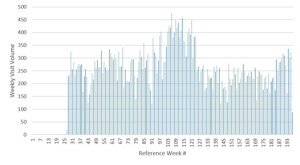
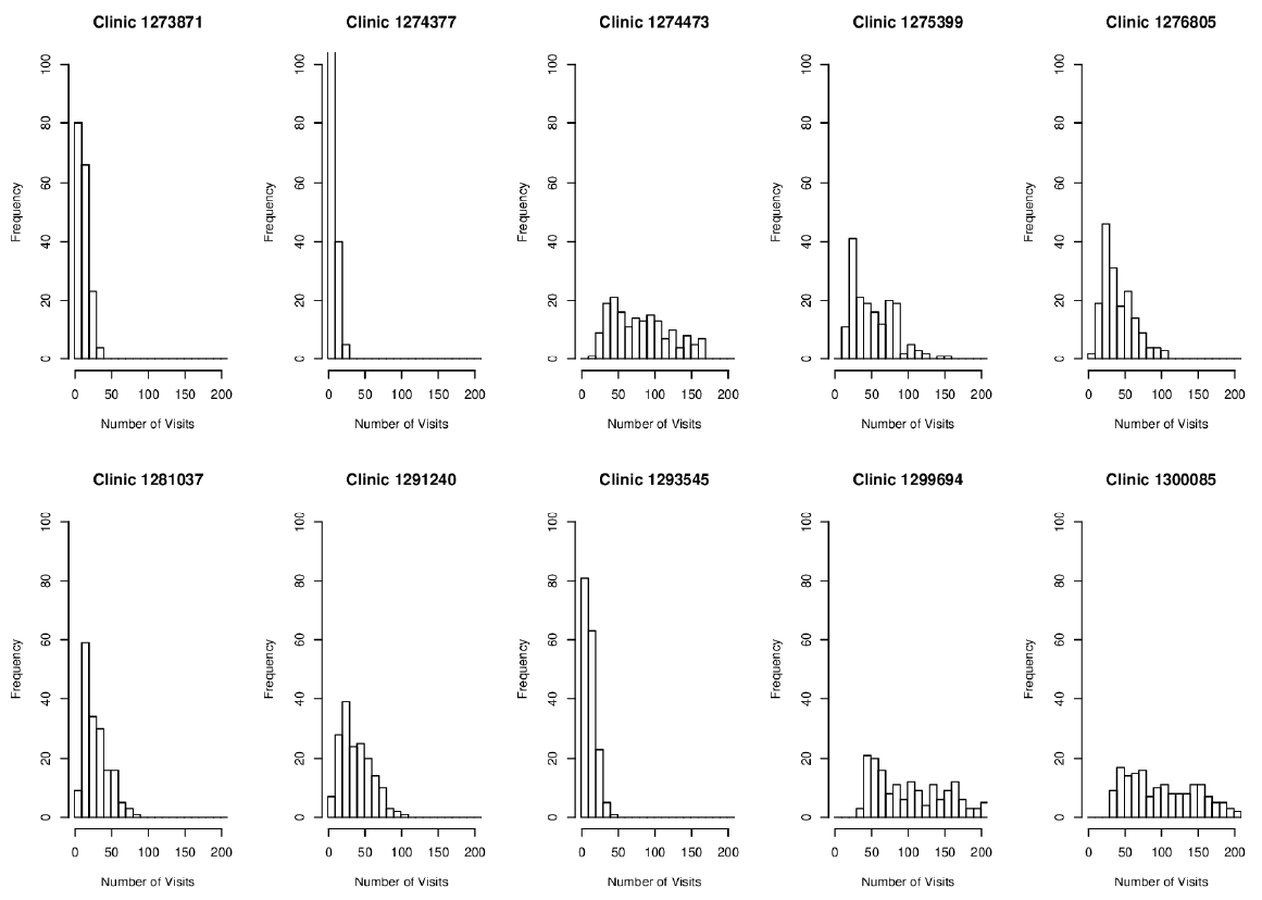
To identify viable outputs from the CRx model, we use empirical data for total weekly visit volumes to 10 select clinics over three years for patients age 16 years and older, obtained from Lindau et al. ( 2016). To control for the natural variation in the observed weekly clinic visit volumes, we manually select stable time regions (periods without visible ramp up or ramp down variations in weekly visit volumes) for each of the 10 clinics, from which we measure the visit statistics (mean and standard deviation) to serve as the target outputs for the same clinics in the CRx ABM. Figure 1 depicts the observed empirical visit volumes for one exemplar clinic, showing the selected stable region. Manual selection of stable regions allows us to avoid tail events, which are outside the scope of our model, as are the seasonality of clinic visits . Table 1 details the mean and standard deviation for stable weekly visit volumes for the 10 clinics of interest, and represent the targeted outputs for the CRx ABM. The 10 clinics were selected from the set of CRx model clinics \(\mathbf{C}\), based on the availability of empirical data from Lindau et al. (2016), after ignoring clinics attached to schools (which have a significant population under 16 and thus out of our model scope), clinics with too few weekly visits to obtain robust statistics (\(< 20\)), and emergency rooms (which included patient visits for reasons other than health maintenance, and thus were out of scope).
| Clinic Code | Mean of Weekly Visits | Standard Deviation of Weekly Visits |
| 1273871 | 267.14 | 74.75 |
| 1274377 | 28.60 | 11.14 |
| 1274473 | 62.50 | 26.47 |
| 1275399 | 241.49 | 88.44 |
| 1276805 | 142.84 | 47.18 |
| 1281037 | 80.56 | 23.90 |
| 1291240 | 80.36 | 26.23 |
| 1293545 | 59.17 | 23.42 |
| 1299694 | 207.79 | 42.61 |
| 1300085 | 204.97 | 43.90 |
The objective function used to characterize the model output calculates the \(z\) score (\(z=\frac{x-\mu}{\sigma}\)) from the model-generated mean clinic visits for each of the 10 clinics during the third week of the model run, against the empirically observed weekly mean and standard deviation (\(\mu,\sigma\)) of visits for these clinics (as specified in Table 1). The model exhibited stable behavior by week 3 (steady-state output seen in the number of weekly visits to the 10 selected clinics,) and thus, we calculate the \(z\) score using data from that period. 1 Considering week 3 instead of a later week, also allowed us to fit in more model evaluations within the same computational budget.
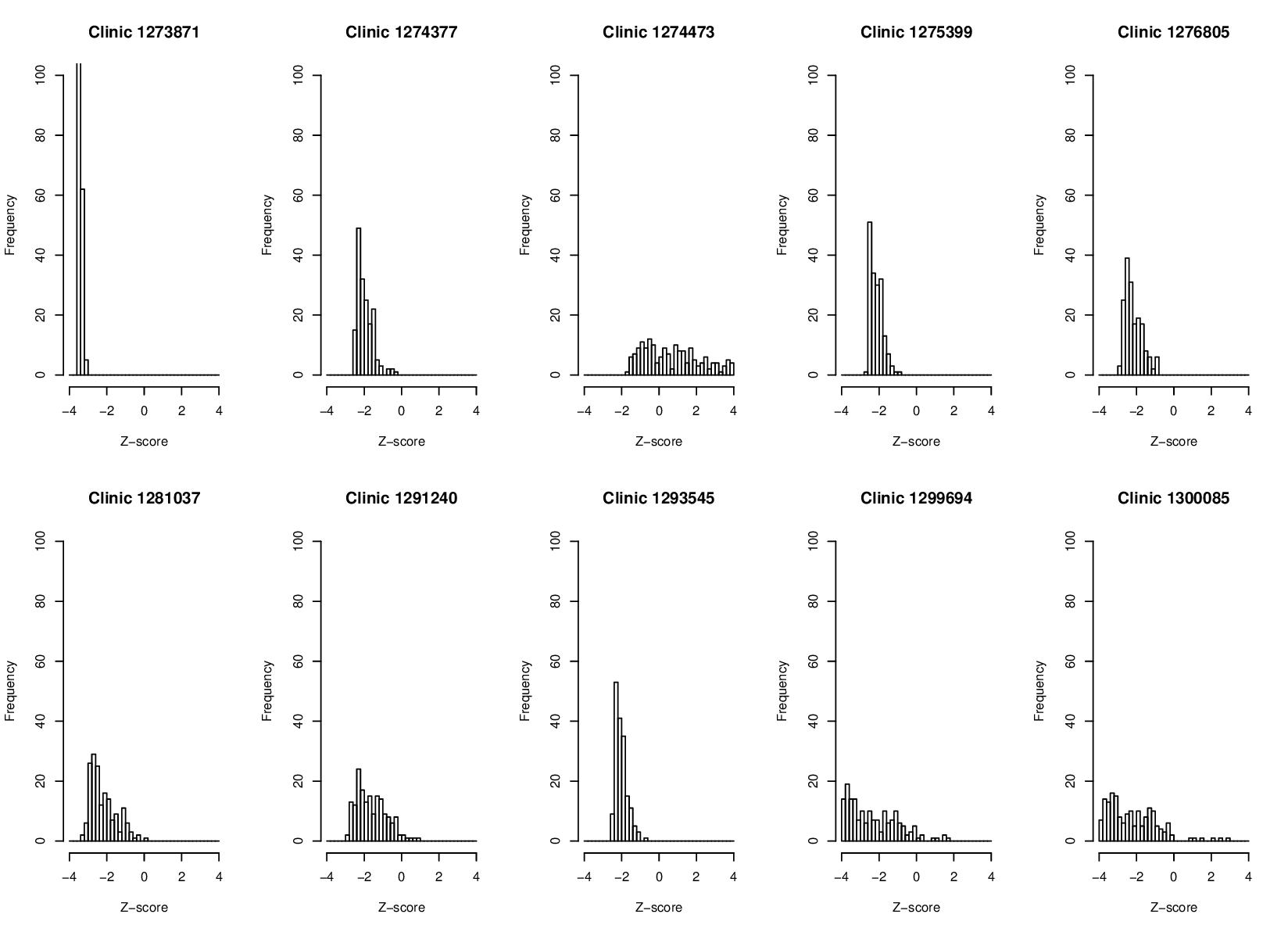
A threshold condition was defined using the z score within which the model outputs are deemed to adequately resemble empirically observed weekly clinic volumes. The threshold condition used was a \(z\) score for each of the 10 clinics in the range of +4 and -4 for the third week of the model run, i.e., \(-4 \geq \frac{x_i^t-\mu_i}{\sigma_i} \geq +4\) where \(x\) is the total number of agents who visited clinic \(i\) (Clinic_Code in Table 1) in week \(t=3\), and (\(\mu_i,\sigma_i\)) are the empirically observed mean and standard deviation for clinic \(i\), as detailed in Table 1. Note that while empirical observations in Table 1 imply that 0 visits to some of these clinics would individually result in a \(z\) score within \((\) -4,+4 \()\) , it, however, does not satisfy our threshold condition. The implemented threshold condition necessitates that all 10 clinics individually satisfy the \(z\) score threshold condition. Figure 16 in Appendix D shows the weekly visit numbers across all clinics across all 173 potentially viable parameter combinations; it is observed that while a low number of visits (<10) account for approximately 20% of observations, there are no zero visits during the week for any of the 10 clinics despite the use of the z-score threshold of +/-4. Figure 2 shows the marginal distributions for the z-scores for each of the 10 clinics across all 173 potentially viable points (refer Figure 17 in Appendix D for marginal distributions of actual visit numbers recorded by the simulation for each of the 10 clinics across all potentially viable parameterizations.) Given our stated goal of characterizing the parameter space into potentially viable and non-viable regions as the initial part of a stepwise tightening of viability constraints, this threshold condition results in a restricted parameter space for subsequent, more constrained model calibration. 2 Appendix D includes additional discussions on the sensitivity of the \(z\) score threshold on potentially viable parameterizations, as well as the stepwise tightening of viability constraints.
CRx ABM parameter space and discretization
Clinic visits by agents within the CRx ABM occur through the decision calculus described in Section 2.4. The implementation of the CRx ABM has several parameters that have the potential to influence agents’ clinic visits (refer to Table 5 in the appendix for a complete list of parameters used in the CRx ABM). For this study, we sub-selected the five most potentially influential parameters in Table 2, based on their potential to directly affect an agent’s decision calculus in Equations 1 and 2, and for which we could not directly infer values from the extant literature. Given the targets for model output, potentially viable regions within the parameter space of the CRx model are regions representing the valid combinations of input parameter values that satisfy the threshold condition defined above.
Given our inability to infer parameter values from empirical data, we utilize an AL model exploration method described in the following sections to identify potentially viable parameter combinations. The AL algorithm that we implemented utilizes a discretization of the parameter space. The algorithm selects from unique parameter points (combinations of parameter values across all dimensions) for evaluation and prediction. We selected 15 discrete points along each parameter dimension to provide a sufficient level of granularity with respect to the model output targets and to be able to show uncertainty gradients between the non-viable and potentially viable regions while keeping within an easily manageable memory footprint for the AL algorithm. 3 For each combination of the five parameters in Table 2 (which represent a unique point in parameter space), the CRx model produces weekly clinic visits for each of the 3 simulated weeks.
| Parameter | Description | Min | Max | Increment |
|---|---|---|---|---|
| dosing.decay | rate of knowledge attrition | \(0.9910\) | \(0.9994\) | \(0.0006\) |
| dosing.peer | dosing from network peer | \(0.8000\) | \(0.9500\) | \(0.1000\) |
| gamma.med | resource inertia of performing an moderate level of activity | \(1.0000\) | \(3.0000\) | \(0.1430\) |
| propensity.multiplier | multiplier applied to propensity of information sharing | \(0.5000\) | \(1.5000\) | \(0.0714\) |
| delta.multiplier | multiplier applied to distance threshold \(\delta_l\), \(\delta_m\) , \(\delta_h\) | \(0.5000\) | \(1.5000\) | \(0.0714\) |
Adaptive sampling methods for ME
Given the targets for model output and threshold condition for determining potentially viable regions for model exploration, the challenge becomes one of computational feasibility. As described earlier, the CRx ABM parameter space consists of \(15^5\) points (each point corresponding to a unique combination of parameter values) across 5 dimensions. Characterizing this parameter space into potentially viable and non-viable regions thus presents a computational challenge – evaluating 759,375 points by brute force methods or producing a sufficiently dense covering of the space is computationally prohibitive. Instead, we strategically sample the parameter space by selectively applying computational budgets to more important regions.
There do exist multiple sampling methods to deal with large parameter spaces, each, however, present their own problems. Grid search methods (dividing the parameter space into equivalent grids), while naturally parallel, suffer from evaluations being made independent of each other, which in high-dimensional parameter spaces can result in high computational costs without corresponding information value. Bergstra & Bengio (2012), for instance, provide empirical and theoretical proof that even random selection is superior to grid selection in high-parameter optimization. Random search, however, is generally not as good as the sequential combination of manual and grid search (Larochelle et al. 2007) or other adaptive methods (Bergstra & Bengio 2012).
Other commonly used a priori sampling methods include orthogonal sampling (Garcia 2000) and Latin Hypercube Sampling (LHS) (Tang 1993). While both methods ensure that sampled points (for evaluation) are representative of overall variability, orthogonal sampling ensures that each subspace is evenly sampled. However, these methods also suffer in high-dimensional spaces, where checking parameter combinations and interactions across all dimensions are computationally costly. The challenge of computational feasibility in large parameter spaces often results in computational compromises, like restricting the fidelity, size or scale of the model, or limiting the types of computational experiments that are undertaken.
An adaptive approach to ME is thus necessary for models with large multi-dimensional parameter spaces, like the CRx ABM. While a number of different adaptive methods, including evolutionary algorithms and ABC could potentially be used (Ozik et al. 2018), an AL approach, described in the next section, maps naturally to the problem. This approach is generalizable and, as we demonstrate in this paper, computationally feasible with new approaches to HPC-scale techniques.
Active learning for ME
We use an AL (Settles 2012) approach to characterize the large parameter space of the CRx ABM, using meta-models (Cevik et al. 2016). The AL method combines the adaptive design of experiments (Jin et al. 2002) and machine learning, to iteratively sample and characterize the parameter space of the model (Xu et al. 2007). In this work, we use the EMEWS framework (described later in Section 4.1), to integrate an R-based AL algorithm, enabling its application at HPC scales, as reported in (Wozniak et al. 2018).
We use an uncertainty sampling strategy in our AL approach. We employ a random forest classifier on already evaluated points and choose subsequent samples close to the classification boundary, i.e., where the uncertainty between classes is maximal, to exploit the information of the classifier. With the availability of concurrency on HPC systems, samples at each iteration of the AL procedure are batch collected (and evaluated) in parallel. Candidate points are first clustered, and an individual point is chosen from this cluster. This approach decreases the overlap in reducing classification uncertainty and ensures a level of diversity in the sampled points (Xu et al. 2007). Each sampling iteration also includes randomly sampled points, striking a balance between the exploitation of information that the classifier provides with an exploration of the parameter space to prevent an incomplete meta-model due to premature convergence.
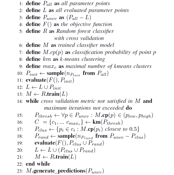
The pseudo-code for our AL algorithm is shown in Figure 3. [AL] Parallel evaluations of the objective function F(), the CRx model simulation, are performed in lines 11 and 19 over a sampling of parameter space. At each iteration, the sampled results are fed into the random forest classifier R (lines 13 and 21). At the end of the workflow, the final meta-model predictions are generated for the unevaluated parts of the parameter space.
Enabling Model Exploration using EMEWS and Parallelization
EMEWS (Extreme-scale Model Exploration with Swift)
As ABMs improve their ability to model complex processes and interventions, while also incorporating increasingly disparate data sources, there is a concurrent need to develop methods for robustly characterizing model behaviors. The EMEWS framework (Ozik et al. 2016) was a response to the ubiquitous need for better approaches to large-scale model exploration on HPC resources. EMEWS, built on top of the Swift/T parallel scripting language (Wozniak et al. 2013) enables the user to directly plugin: 1) native-coded models (i.e., without the need to port or re-code) and 2) existing ME algorithms implementing potentially complex iterating logic (e.g., Active Learning Settles 2012). The models can be implemented as external applications accessed directly by Swift/T (for fast invocation), which is the method that was used in this work. However, applications can also be invoked via command-line executables, or Python, R, Julia, JVM, and other language applications via Swift/T multi-language scripting capabilities. ME algorithms can be expressed in the popular data analytics languages Python and R. We implemented an R-based Active Learning ME algorithm for this work. Despite its flexibility, an EMEWS workflow is highly performant and scalable to the largest cutting-edge HPC resources. This large-scale computation capability provided us the ability to efficiently characterize the parameter space of the CRx ABM and discover parameter space regions compatible with empirical data.
Parallelization to enable model exploration
The CRx model is a computationally expensive application, primarily due to the interactions between the large number of agents and places. At each time step, every agent in each place can potentially share information with every other person in that place. In the absence of any parallelization, this entails iterating over each place in the model in order to iterate over all the agents in that place so that each person can share information with every other person in that place. In order to mitigate this expense and reduce the run time such that adaptive model exploration was feasible, we parallelized the model both across and within compute cores.
Inter-process parallelization
The model was parallelized across compute processes using the chiSIM framework (Macal et al. 2018). chiSIM-based models such as CRx are MPI applications in which the agent population and the agents’ potential locations are distributed across compute processes, that is, across MPI ranks. Each process corresponds to an MPI rank and is identified with a rank id. Agents move across ranks while places remain fixed to a particular rank. A chiSIM model’s time step consists, at the very least, of each agent determining where (i.e., what place) it moves to next and then moving to that place, possibly moving between process ranks in doing so. Once in that place, some model specific co-location dependent behavior occurs, for example, disease infection dynamics, or in the case of CRx, information sharing. The model code runs in parallel across processes and thus the iteration over each of the 482,945 places in the model described above becomes n number of parallel iterations over p number of places, where n is the number of process ranks, and p is the number of places on that rank.
The success of this cross-process distribution is dependent on how well the process loads are balanced. Too many places or agents on a process results in a longer per time step run time for that process and other processes sitting idle while that slower process finishes. In addition, we also want to minimize the potentially expensive cross-process movement that occurs when agents move between places on different process ranks. Our load balancing strategy described in detail in Collier et al. (2015), uses the Metis (Karypis & Kumar 1999) graph partitioning software to allocate ranks to processes, balancing the number of agents per rank while minimizing cross-process movement. The movement of agents between places can be conceptualized as a network where each place is vertex in the network and where an edge between two places is created by agent movement between those two vertices. It is this network that Metis partitions. In previous work, (Macal et al. 2014) and (Ozik et al. 2018), this movement was dictated by relatively static agent schedules and the network was created directly from those schedules without having to run the model itself. In the CRx case, agents’ movement schedules are selected at random every simulated day from a demographically appropriate set of schedules. In the absence of a static schedule , we ran the model for 14 simulated days in order to capture the stochastic variation in agent movement, logging all individual agent movements between places. These data were then used to create the weighted place-to-place network for Metis to partition using the strategy outlined in Collier et al. (2015).
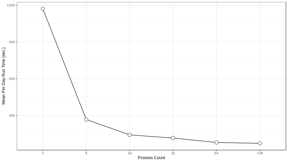
We experimented with distributing the model over different numbers of ranks - 1, 8, 16, 32, 64 and 128 - running the model for a simulated week and recording the run time to execute each simulated day. These experiments were performed on Bebop, an HPC cluster managed by the Laboratory Computing Resource Center at Argonne National Laboratory (further details on the Bebop cluster are given in Section 4.4). The results can be seen in Figure 4 . Performance does not scale linearly, which is to be expected given the overhead of moving agents between process ranks. The intention here is to achieve good enough performance such that the model exploration can be run within the maximum job run time, memory, and node count constraints of our target HPC machines. In that respect, the 64 or 128 rank configurations are sufficient. We utilize the 128 rank configuration for the AL workflow described below.
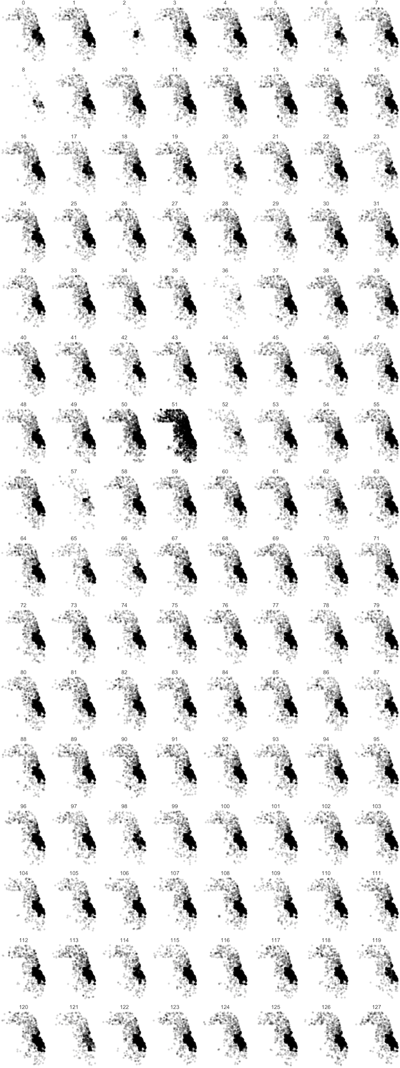
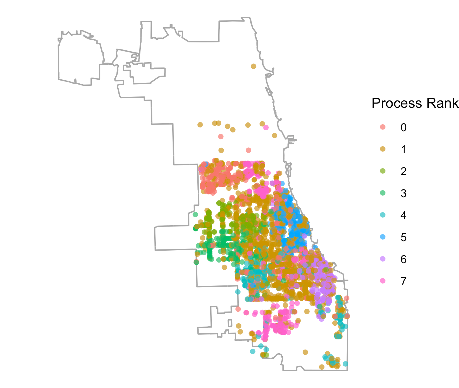
We were also interested in how the model distribution related to the geographic distribution of places across process ranks. This was prompted by previous attempts in the literature to distribute ABMs geographically (Lettieri et al. 2015), where it was determined that geographically based model distribution presented difficulties in achieving performance gains based on the uneven density of agent populations and, as a result, agent activities. In Figure 5 we show all places across Chicago, including households, schools, workplaces, and services, assigned to each process rank in the 128 rank configuration (while we restricted the synthetic population to 16 zip codes, we included places across all Chicago locations). While there are differences in the patterns observed across ranks, one cannot readily detect any process-specific geographic clustering. This observation strengthens the argument against regarding geographic extents as natural partitions for load balancing when complex travel patterns across geographic regions are involved. However, we do know that the information on the HRxs distributed to our agents is based on geographic proximity to the agent household location. Hence, we could expect that, through geographically local information exchanges between agents engaging in geographically local activities at service providers, the information about service providers could retain some locality. In fact, we do see a correspondence between the geographic location of a service and its process rank in Figure 6, using the 8 rank configuration for clarity. This suggests that the location of services and the information flow about them produce correlations in agent movement between them that, in turn, create useful partitions for model load balancing.
Intra-process parallelization
In addition to parallelizing the model by distributing it across processes, we also experimented with intra-process parallelization by multi-threading the model using the OpenMP
(Dagum & Menon 1998)
application programming interface. In distributing the model across processes, we effectively reduced the number of agents and places on each process. And thus, the loop iteration through all the places in the model that occurs every time step was that much smaller (i.e., faster) and occurred in parallel. Intra-process parallelization with threads used the openMP pragma directive
#pragma omp parallel for
to iterate through this loop in parallel. An
omp parallel for
essentially divides the range spanned by the loop into some number of sub-ranges, each sub-range then executes the code within the loop on a separate parallel thread.
However, this code executed in the loop iteration discussed above contains many random draws from a shared random stream. In a multi-threaded context, this could, and in fact most certainly would, lead to race conditions, stream corruption and application crashes, for example, when one thread is drawing from the stream while another is simultaneously updating the stream after its random draw. There are sophisticated strategies for implementing parallel random streams in simulations (see for example Freeth et al. 2012), but we implemented a simpler solution. OpenMP provides a function call to retrieve a running thread’s unique numeric id. On model initialization we created a number of random streams equal to the number of threads and associated each with a thread’s unique id, allowing each thread to retrieve its own random number stream by thread id.
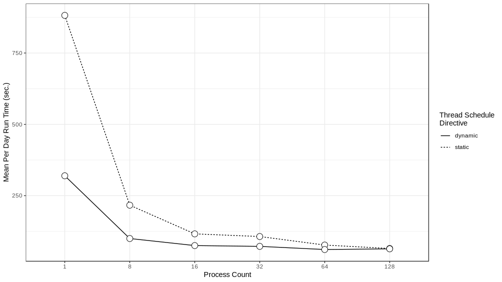
We ran the multi-threaded version of the model, again distributed over different numbers of ranks, setting the number of threads to 6, and using two different threading schedule directives:
static
(the default) and
dynamic
. With the
static
directive each thread is assigned a chunk of the total number of iterations in a fixed fashion and iterations are divided equally among threads. With the
dynamic
directive, each thread is assigned an iteration when that thread becomes available for work. Six threads were chosen as the best tradeoff between how many cores to allocate to a process for individual threads and how many processes to pack into a HPC node (a collection of cores). The results of these runs can be seen in
Figure
7.
In all of the cases, we can see that the
dynamic
directive runs are the fastest for the same number of ranks and that the difference between
static
and
dynamic
run times is especially prominent in those runs that were distributed over smaller number of ranks. This difference is likely due to the non-uniform distribution of agents among places. For example, a typical household may have 4 or so agents in that household, while a larger workplace or clinic may have much more. Given that the length of time it takes to iterate through all the places assigned to a particular thread is dependent on the number of agents in those places, a thread that contains places with larger numbers of agents takes longer to complete when compared to a thread with places with fewer numbers of people. The
dynamic
directive naturally load balances the place iteration by assigning a place to a thread when a thread is available for work. Consequently, while places that require a longer runtime will occupy a thread for a while, other threads are still capable of accepting new places, resulting in a more even spread of work across all the threads. The drawback of the
dynamic
directive is that the order of random draws is now no longer predictable but rather dependent on run time and the threading library, and as a result, we cannot be sure that runs using the same random seed will necessarily produce the same results. We hope to examine this issue of run reproducibility under different threading regimes (static, dynamic, and others) in future work.
AL Results
In this section, we first evaluate the relative importance of 5 model parameters, describe the evolution of the AL algorithm across iterations, present the parameter space characterization results of the CRx ABM and report on the meta-model performance. The AL runs were performed on the Cray XE6 Beagle at the University of Chicago, hosted at Argonne National Laboratory, and on the Bebop cluster, managed by the Laboratory Computing Resource Center at Argonne National Laboratory. Beagle has 728 nodes, each with two AMD Operton 6300 processors, each having 16 cores, for a total of 32 cores per node. Each node has 64 GB of RAM. Bebop has 1024 nodes comprised of 672 Intel Broadwell processors with 36 cores per node and 128 GB of RAM and 372 Intel Knights Landing processors with 64 cores per node and 96 GB of RAM. Additional development was done on the Midway2 cluster managed by the Research Computing Center at the University of Chicago. Midway2 has 400 nodes, each with 28 cores and 64 GB of memory. The AL parameter space characterization runs were executed in 4 rounds. The first round consisted of an LHS sweep used to seed the first AL round (see Section
5.4), followed by 3 AL rounds. The second and third AL rounds were restarted from the serialized final state of the AL algorithm from the previous round. Each of the 4 rounds was run on 215 nodes with 6 computational processes per node. The LHS sweep ran for 85 hours. AL Rounds 1 and 2 ran for 48 hours, and the 3rd AL round for 47 hours for a total of 228 hours (1,764,720 total core hours) for all 4 rounds. Each model run was distributed over 128 processes and was allocated 4 threads per process using the
static
threading directive. The combination of inter- and intra-node parallelism provides an estimated 18-fold runtime speedup from the base undistributed and unthreaded model.
Parameter importance
The random forest classifier is an ensemble of decision trees, where each tree is trained on a subset of the data and votes on the classification of each observation, variable importance can be calculated from the characteristics of decision trees. Two commonly used measures for importance are: the mean accuracy decrease, which is a measure of mean classification error, and the mean decrease in Gini, which is a measure of the weighted average of a variable’s total decrease in node impurity (which translates into a particular predictor variable’s role in partitioning the data into the defined classes). A higher Gini decrease value indicates higher variable importance and vice versa. Table 3 shows an analysis based on these two metrics for our results.
| variable | assigned dimension id | accuracydecrease | Ginidecrease | ||
|---|---|---|---|---|---|
| gamma.med | d1 | 0.306 | 244.660 | ||
| delta.multiplier | d2 | 0.309 | 210.093 | ||
| propensity.multiplier | d3 | 0.184 | 115.937 | ||
| dosing.decay | d4 | 0.230 | 112.647 | ||
| dosing.peer | d5 | 0.174 | 117.695 |
Based on these results we assign the following designations in order of relative parameter importance: \(d1 := gamma.med\), \(d2 := delta.multiplier\), \(d3 := propensity.multiplier\) , \(d4 := dosing.decay\) and \(d5 := dosing.peer\). We use this relative ordering of parametric importance to organize the visualizations of our results in the following sections.
Characterization of CRx ABM parameter space with active learning
The AL algorithm was seeded with the results of 240 evaluations where the sampled points (to evaluate) were selected via a Latin Hypercube Sampling. At each iteration step, 20 new points are evaluated, 10 points close to the classification boundary (exploitation) and 10 randomly sampled points (exploration); the class (i.e., potential viability or non-viability) of each parameter point is determined using its z-score as previously described (to statistically match the empirically observed clinic visits). Following the evaluations, the random forest model is updated with this new class information and generates predictions for out-of-sample (non-evaluated) points across the remaining parameter space. Following 58 iterations, the AL algorithm evaluated a total of 1400 unique points.
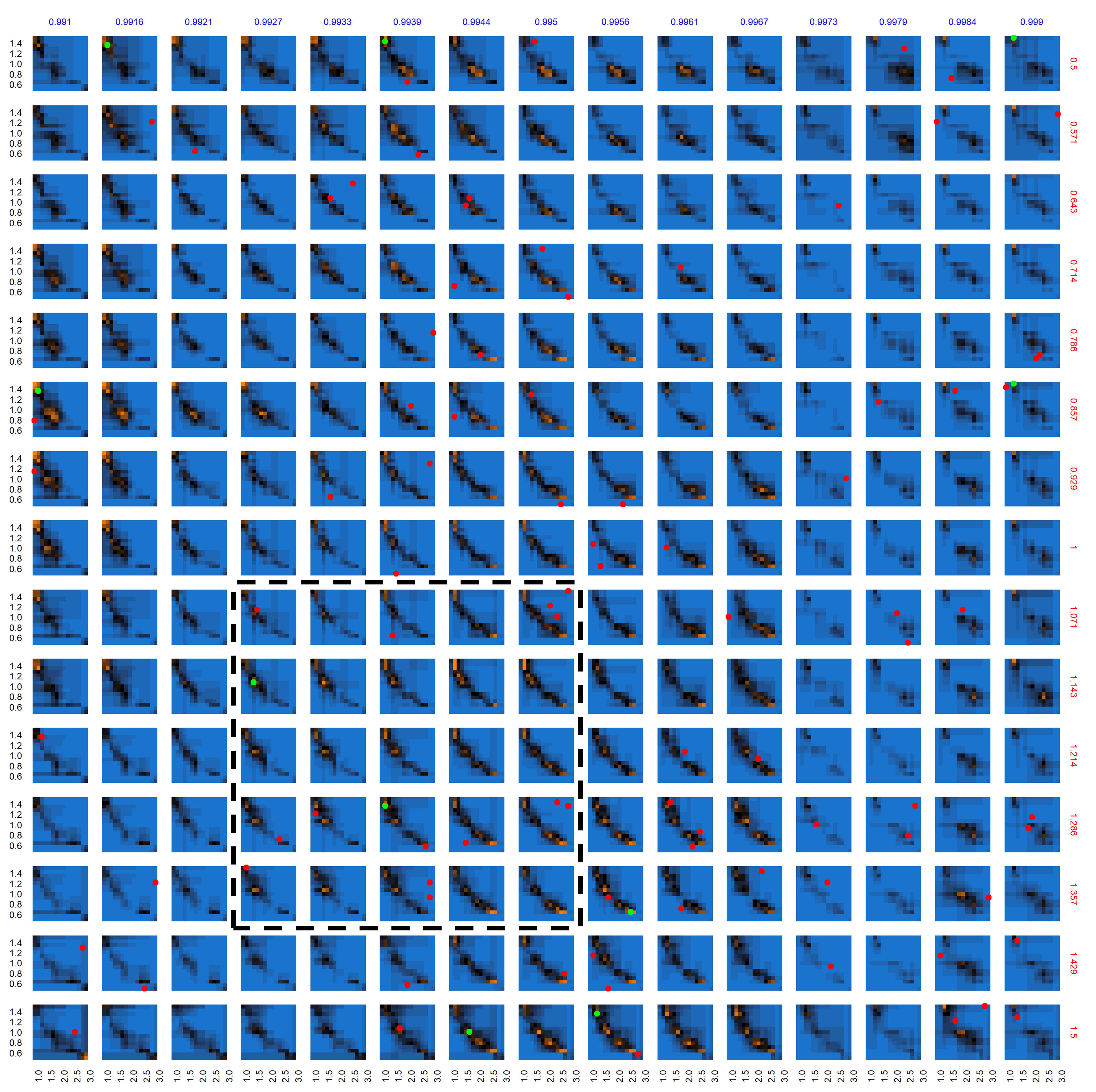
The characterization (evaluated points and predictions for out-of-sample points) of this multi-dimensional parameter space following the AL workflow after 58 iterations is shown in Figure 8. Figure 8 provides a view into the 5-dimensional parameter space through a grid of 2D plots. Each cell in the grid plots the two most relevant dimensions, gamma.med (d1, x-axis) and delta.multiplier (d2, y-axis), against each other. The propensity.multiplier (d3) is varied across the overall rows and dosing.decay (d4) across the overall columns. The final dimension, dosing.peer (d5), is kept constant. Figure 8 thus represents a slice of 5-dimensional parameter space with 225 snapshots of d1 \(\times\) d2 across 15 unique values each for d3 and d4, for a fixed unique value of d5 (0.907). Evaluated points are shown in red/green dots indicating non-viable / potentially viable points. Out of sample predictions are shaded as blue (non-viable), orange (potentially viable), and black (equiprobable), where the color gradient between blue to black to orange denotes the varying probability of classification.
Evolution of parameter space characterization across AL iterations
Figure 9 shows the progression of the AL algorithm for the subset of panels shown in Figure 8 within the dashed bounding box, demonstrating the evolution of evaluated points and the corresponding random forest model predictions for out-of-sample points. We see in Figure 9 that as the AL progresses across the four sets of panels (representing almost-equally spaced iterations 0, 19, 38 and 58), the initial prediction boundary (black regions) is gradually refined as additional points are evaluated across the iterations, while the meta-model prediction for the rest of the parameter space (blue/orange regions depicting the non-viable / potentially viable predictions) is clarified with less uncertainty in the model prediction.
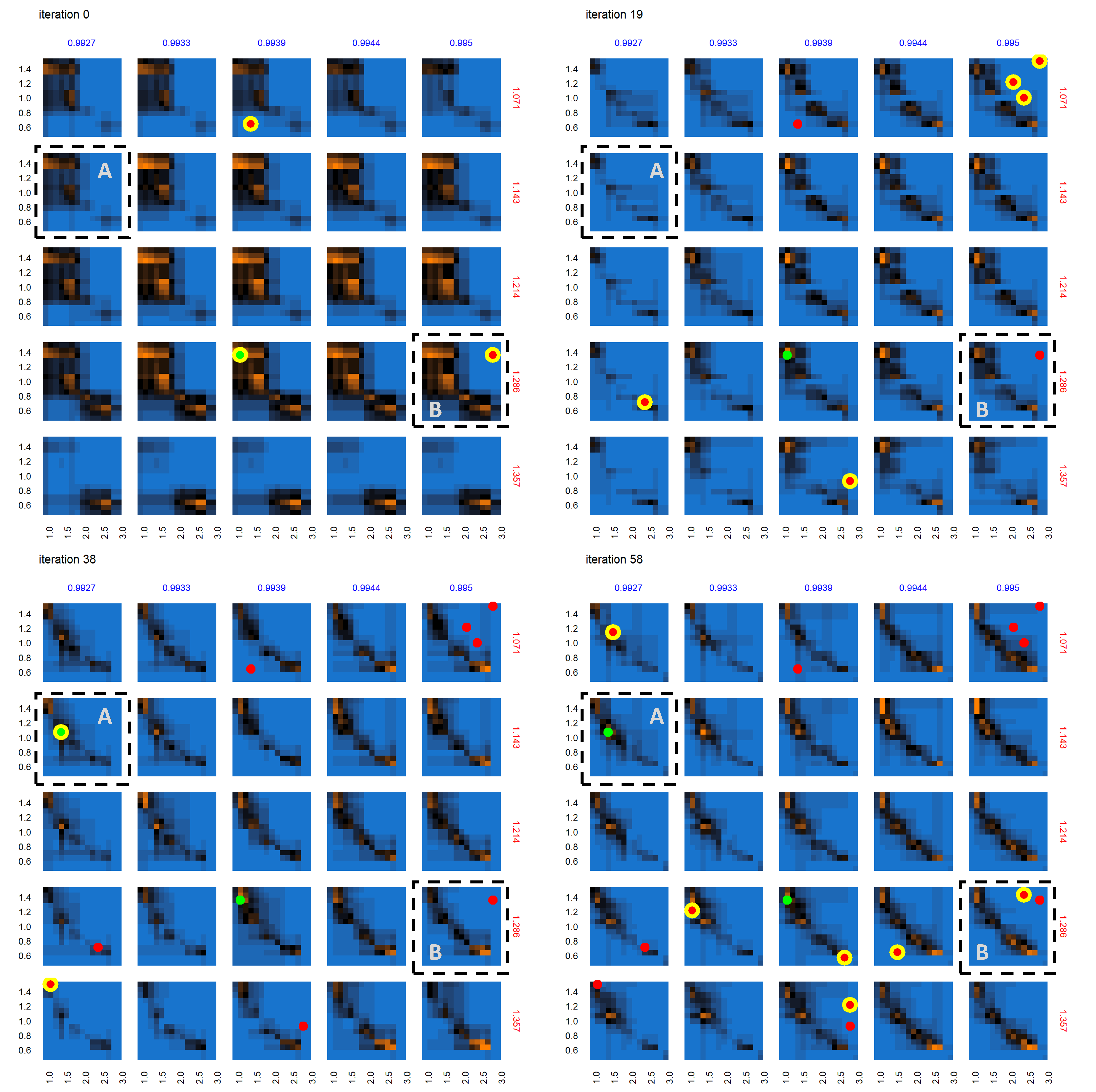
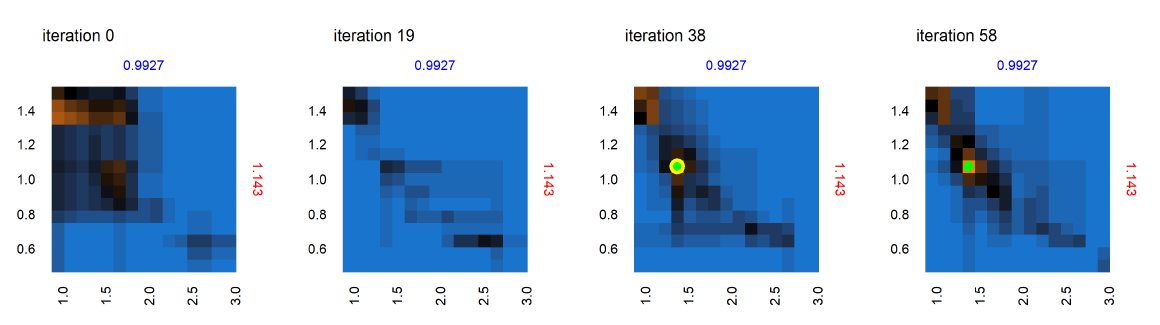
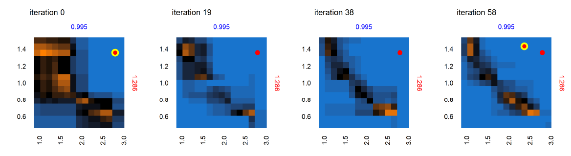
Next we consider the panel labeled A in the set of panels corresponding to iteration 0 in Figure 9 – shown in Figure 10 , across iterations 0, 19, 38 and 58. At iteration 0 and 19 in Figure 10, while no point was yet positively evaluated, we still see an evolution of the meta-model predictions for out-of-sample regions. There is a positive evaluation by iteration 38 (green point with yellow halo), and we observe that as a result of the positive evaluation, the meta-model prediction for the potentially viable regions (orange) in the parameter space around this point has been refined with increased certainty (increased color intensity). Figure 11 features the individual panel labeled B in Figure 9, also across iterations 0, 19, 38 and 58. We see new points in iteration 0 and iteration 58 evaluated as non-viable (red dots with yellow halo). It is also observed that regions of parameter space with high uncertainty (black regions) decrease in width and area, sharpening the distinction between non-viable and potentially viable (blue/orange) regions. Figure 11 thus shows reduced uncertainty about the non-viable regions following a negative evaluation.
Parameter space evaluation and meta-model performance
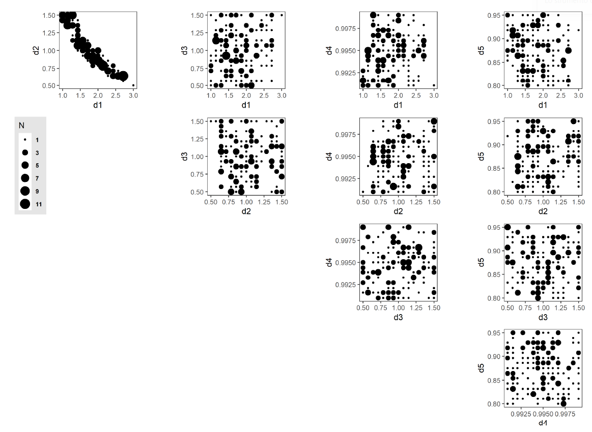
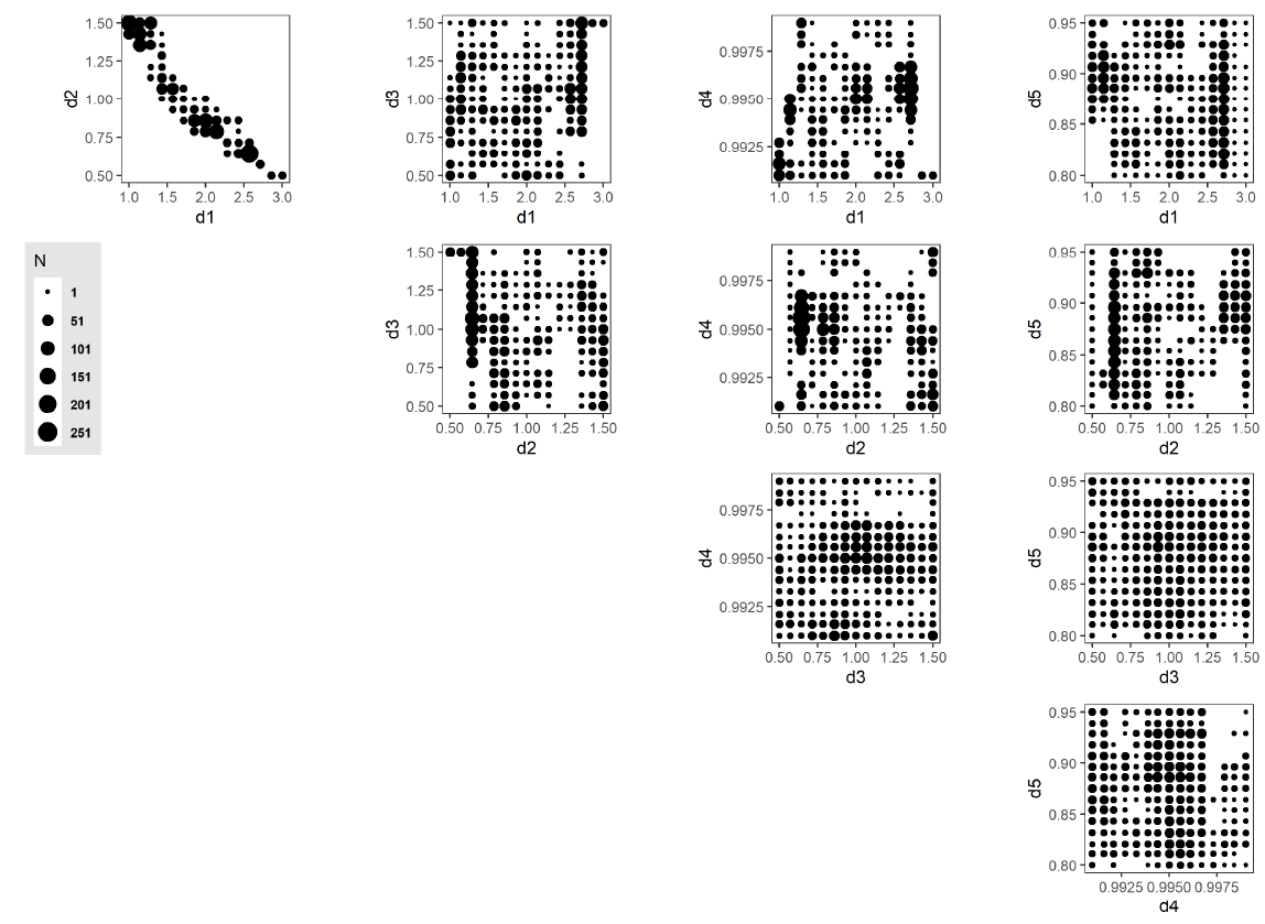
The AL algorithm evaluated a total of 1400 unique points in the discretized parameter space (out of a total of 759,375 possible points) after 58 iterations. Of these,173 points were classified as potentially viable, and are presented in Figure 12, with point sizes indicating the number of unique points at each collapsed 2-dimensional space point. One aspect to note is the strong correlation exhibited between parameters d1 and d2 and the sharp boundary within the parameter space that this produces. This observation shows an inverse relationship between the parameterization of resource inertia for moderate activities (d1) and the multiplier applied to the distance threshold (d2). This observed relationship suggests that this interplay between activity difficulty and distance to a resource is the primary driver within the set of five selected model parameters in determining resource use at the population level. Table 6 lists all 173 points.
To analyze the performance of the random forest meta-model in classifying out-of-sample (non-evaluated) parameter space, we train the random forest algorithm on the evaluated points. Using a 3-fold cross-validation training method, we determine the Positive Predictive Value (PPV) measure of our meta-model prediction (Altman & Bland 1994a, 1994b). PPV is the proportion of true positives to the total positive classifications, i.e., \(PPV=\frac{\text{True Positive}}{\text{True Positive} + \text{False Positive}}\). As PPV increases, we increase our certainty that a point classified as \(X1\) is a True Positive.
The classification of a point in the parameter space is a mapping function \(f:s\to\{X0,X1\}\), of a probability score \(s\) assigned by the trained meta-model, to a classification class (\(X0\) or \(X1\)), based on a threshold measure (Lipton et al. 2014) \(p_t\) , such that \(f = X1 \ \text{for} \ s\geq p_t, X0 \ \text{otherwise}\). Table 4 shows the PPV against different thresholds as well as the expected number of \(X1\) classified points in the non-evaluated parameter space, for each threshold. We observe that higher thresholds result in higher PPV, but with smaller total numbers of points classified as \(X1\). As the threshold increases, the meta-model generates more False Negatives in exchange for a higher rate of True Positives. We chose a threshold of 0.9 for the meta-model.
| Threshold | Positive Predictive Value | Number of \(X1\) Points |
|---|---|---|
| 0.50 | 0.480 | 30056 |
| 0.60 | 0.550 | 18246 |
| 0.70 | 0.630 | 10592 |
| 0.80 | 0.740 | 5392 |
| 0.90 | 0.860 | 2212 |
As mentioned earlier, the random forest model predicted potentially viable points from the out-of-sample region (the remaining 757,975 non-evaluated points) with an associated probability, ranging from 0.0 (non-viable) to 0.5 (equiprobability of classification) to 1.0 (potentially viable). 2212 potentially viable points are predicted from the out-of-sample region when considering a 0.9 threshold probability; these are shown in Figure 13.
The set of 173 potentially viable points ( Figure 12) and 2,212 predicted potentially viable points (Figure 13) identifies the region in the parameter space of the CRx model where further investigations are warranted. That is, the main contribution of these points is in characterizing the rest of the parameter space as non-viable, thereby avoiding the expenditure of unnecessary computing resources on other regions, i.e., those not likely to yield empirically corresponding model outputs. These subsequent analyses can use, e.g., stepwise tightening of viability thresholds or surrogate model-based optimization approaches to yield model outputs that are better aligned with empirical observations. As the model calibration is improved, the CRx ABM can increasingly be applied to CRx intervention scenarios as a computational laboratory to conduct in silico experimentation and drive implementation policy (for instance, identifying the most effective delivery mode, or ideal number of clinics to effect an increase in resource recall).
Conclusion
As techniques for building ABMs become more sophisticated and the ABMs become more complex, it has become increasingly difficult to produce trusted tools that can be used to aid in decision and policy making. This is partly due to the computational expense of running large (e.g., urban-scale) models and partly due to the size of the model parameter spaces that need to be explored to obtain a robust understanding of the possible model behaviors. These two issues exacerbate each other when iterative parameter space sampling techniques are utilized to strategically sample the parameter spaces since iterative algorithms require at least some form of sequential evaluation of potentially long-running simulations.
In this work, we presented an urban-scale distributed ABM of information diffusion built using the Repast HPC and chiSIM frameworks. Describing the application of a large-scale AL method, we characterize the parameter space of the CRx ABM to identify a sampling of potentially viable points, while characterization of the rest of the parameter space as non-viable. In the process, we developed intra-node and inter-node parallelization and load balancing schemes to enable an estimated 18-fold runtime speedup. The load balancing was done using the place-to-place agent-movement network, which produced geographic clustering of service providers, understood to be a demonstration of the local nature of resource information sharing between the agents.
With the increased efficiency achieved through parallelization in running individual models, we were able to consider an iterative algorithm for characterizing the model parameter space. We exploited the polyglot and pluggable architecture of EMEWS framework and implemented an R-based random forest Active Learning algorithm, and ran it on 215 nodes of a HPC cluster to calibrate the CRx ABM. The run produced 173 potentially viable parameter combinations through direct evaluation and an additional 2212 parameter combinations inferred to be potentially viable, with an estimated 86% PPV, by a random forest model trained on the evaluated points.
The parameter space characterization that was enabled by our approach represents one component of a comprehensive and iterative model development and validation cycle. Relative to the extant literature on model calibration (Section 3.1) and sequential sampling (Section 3.11), this paper presents the use of Active Learning as part of sequential model-based calibration methods, as seen in (Edwards et al. 2011; Holden et al. 2018), for large scale parameter space exploration. The combination of AL and parallelization techniques (described in Section 4.2) enables model exploration in simulators with large parameter spaces and helps mitigate (Bellman 1961)’s curse of dimensionality. Another important aspect for model validation is the establishing of plausibility for the mechanisms (Edmonds et al. 2019) at multiple model scales, including the parameterization of agent attributes, decision making, and behaviors. The conception of the CRx ABM originated after a discovery by experts in medicine about the spread of information, that was not adequately captured, assessed, or analyzed using individual-level models. The demonstrable and empirical need for an ABM ensured a close collaboration.
In jointly developing the CRx ABM, we have repeatedly incorporated assessments of domain experts on model design, mechanisms, and results, and, perhaps most importantly, these inputs have been sought and incorporated from the early model design stage. The CRx ABM is an additional analytic tool for public health officials who are adopting new technologies such as geospatial statistics and predictive modeling. Potential users of these models include other academics, local and state public health departments, federal agencies such as the Centers for Disease Control and Prevention, health care systems, and health care payers. In the highly decentralized public health system of the U.S., open-source analytic tools that can capture and evaluate the interaction between service entities and community members are needed more than ever.
One limitation of the present work is the potential bias resulting from excluding seasonality in agent behaviors to account for fluctuations in empirical clinic visit data. Furthermore, in order to simplify the scope of the parameter space characterization and produce meaningful results with the computational allocations we had access to, the five model parameters in Table 2 were selected based on expert opinions on model parameters deemed to be most relevant to agent clinic visits. However, this process may have omitted additional parameters with significant effects.
For future work, the CRx ABM (with the potentially viable parameter points) can be used as a starting point on which to focus computing resources to tighten the viability thresholds and identify better-calibrated points, allowing us to use the CRx ABM to expand our investigations into the effects of information spread on population health outcomes. These analyses may also find that structural modifications are needed to align the model with empirical data more closely. Additional model exploration algorithms can also be examined, particularly those that have the ability to incorporate stochastic noise from model replicates, e.g., sequential design with Gaussian Processes (Binois et al. 2018), for producing robust uncertainty estimates of model outputs. Additionally, in order to be able to include larger parameter spaces for our computational experiments, the application of dimensional reduction techniques can be investigated, e.g., active subspaces (Constantine 2015). Finally, we aim to continue expanding our approaches to improved model efficiency and look at reproducibility under different intra-node threading regimes.
The methods we describe in this paper enable computation at HPC scale. A direct potential application of such methods is particularly relevant to public health emergencies like the COVID-19 pandemic, where empirically-informed large scale models can help aid and inform public health authorities in decision-making. Our current research efforts extending some of the methods described in this paper and in (Ozik et al. 2018) involve modeling the spread of COVID-19 in Chicago. A subset of the authors (Macal, Ozik, Collier, Kaligotla) built the CityCOVID ABM, also based on the ChiSIM framework (Macal et al. 2018), which incorporates COVID-19 epidemiology and spread among the 2.7 Million people in the City of Chicago and across 1.2 Million geographical locations. We calibrate our model with daily reported hospitalizations and deaths. Model results are being provided to the City of Chicago and Cook County Public Health Departments as well as the Illinois Governor’s COVID-19 Modeling Task Force. Our work contributes to the growing need for empirically-informed models using granular, local, and time-sensitive data to support decision-making during and in advance of public health and other crises.
Notes
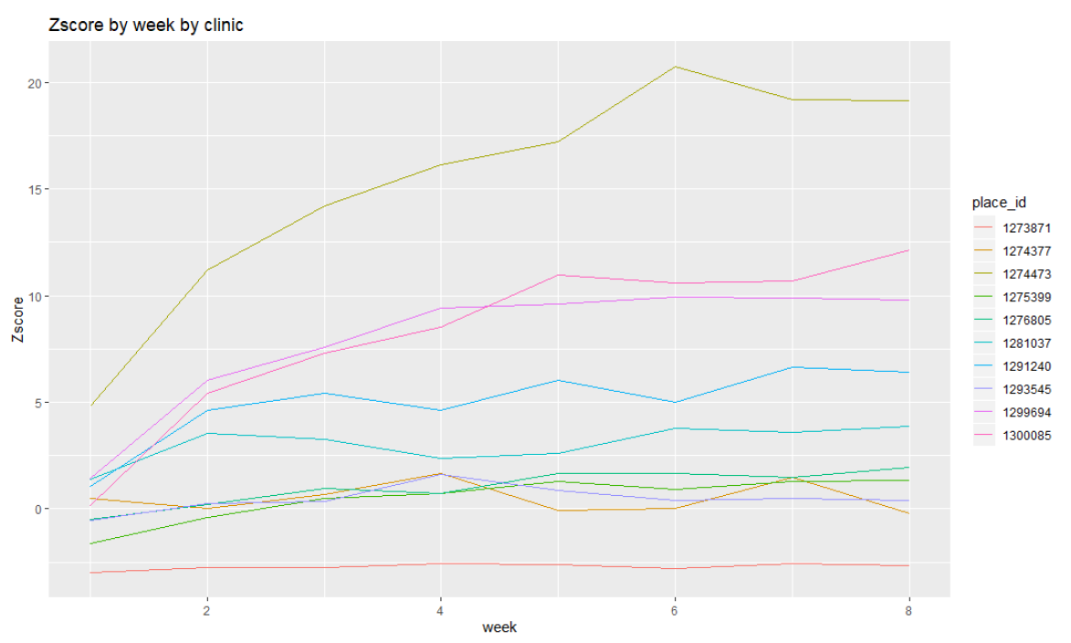
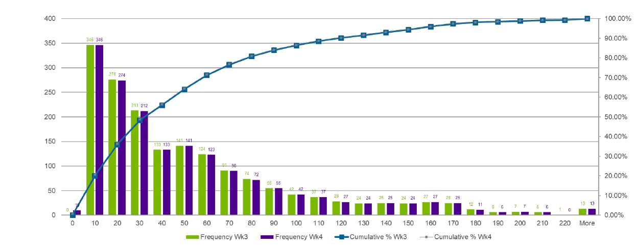
-
Figures 14 and 15 in Appendix D depict model output. Figure 14 shows the z scores from uncalibrated simulated weekly visits for each of the 10 clinics over 8 weeks, while Figure 15 compares the distribution of the total number of weekly visits in Week 3 and Week 4 of the calibrated simulation output.
-
See, e.g., Rutter et al. (2019) for a description of the benefits of employing a stepwise narrowing of thresholds approach instead of narrower initial thresholds.
-
While this discretization was chosen for the current work, it is possible that either a less or a more granular representation could provide useful insights as well. Investigations of optimal discretization for the CRx model is a possible future area of work.
Model Documentation
A comprehensive model description of the CRx ABM is described in (Kaligotla et al. 2018). The CRx ABM model is implemented using the Repast for High Performance Computing (Repast HPC) (Collier & North 2013) and the Chicago Social Interaction Model (chiSIM) (Macal et al. 2018) toolkits. The CRx ABM model code and the workflow code used to implement the parameter space characterization experiments are publicly available (at the following URL: https://github.com/jozik/community-rx).
Acknowledgments
Research reported in this publication was supported by the National Institute on Aging of the National Institutes of Health R01AG047869 (ST Lindau., PI). This content is solely the responsibility of the authors and does not necessarily represent the official views of the National Institutes of Health’s National Institute on Aging. This work is also supported by the U.S. Department of Energy under contract number DE-AC02-06CH11357. This work was completed in part with resources provided by the Research Computing Center at the University of Chicago (the Midway2 cluster), the Laboratory Computing Resource Center at Argonne National Laboratory (the Bebop cluster), and the University of Chicago (the Beagle supercomputer).Conflicts of Interest: ST Lindau directed a Center for Medicare and Medicaid Innovation Health Care Innovation Award (1C1CMS330997-03) called CommunityRx. This award required the development of a sustainable business model to support the model test after award funding ended. To this end, S. T. Lindau is the founder and co-owner of NowPow LLC and President of MAPSCorps, 501c3. Neither The University of Chicago nor The University of Chicago Medicine is endorsing or promoting any NowPow or MAPSCorps entity or its business, products, or services.
Appendix
A: Model parameters
| Model Parameters | Description | Values / Range |
|---|---|---|
| alpha \((\alpha)\) | Activation level | \(\in(0,1)\) Derived from (Skolasky et al. 2011) |
| delta \((\delta_{l},\delta_{m},\delta_{h})\) | Distance threshold (low,med,high) | \(\delta_{l}=1;\ \ \delta_{m}=2;\ \ \delta_{h}=3\) |
| \(delta.multiplier\) | multiplier applied to distance threshold | \(\in(0.5,\dots,1.5)\) in increments of \((0.0714)\) |
| gamma.low \(\left(\gamma_{low}\right)\) | resource inertia of performing an easy activity | \(=1\) |
| gamma.med \(\left(\gamma_{med}\right)\) | resource inertia of performing a moderate activity | \(\in(1,\dots,3)\) in increments of \((0.143)\) |
| gamma.high \(\left(\gamma_{high}\right)\) | resource inertia of performing a difficult activity | \(=3\) |
| propensity \((pr_{none},pr_{l},pr_{m},pr_{h})\) | propensity of information sharing (none,low,medium,high) | \(pr_{none}=0.0001, pr_{l}=0.005,\ \ pr_{m}=0.025,\ \ pr_{h}=0.01\) |
| \(propensity.multiplier\) | multiplier applied to \(p.score\) | \(\in(0.5,\dots,1.5)\) in increments of \((0.0714)\) |
| \(dosing.decay\) \((\lambda)\) | Rate of knowledge attrition | \(\in(0.9910,\dots,0.9994)\) in increments of \((0.0006)\) |
| \(dosing.doctor\) \(\left(\epsilon_{doctor}\right)\) | dosing from doctor | \(0.05\) |
| \(dosing.nurse\) \(\left(\epsilon_{nurse}\right)\) | dosing from nurse | \(0.15\) |
| \(dosing.psr\) \(\left(\epsilon_{psr}\right)\) | dosing from patient service representative | \(0.25\) |
| \(dosing.use\) \(\left(\epsilon_{use}\right)\) | dosing from use of resource | \(0.2\) |
| \(dosing.peer\) \(\left(\epsilon_{peer}\right)\) | dosing from network peer | \(\in(0.8,\dots,0.95)\) in increments of \((0.1)\) |
| \(dosing.kappa\) \(\left(\kappa\right)\) | dosing value for initialization | \(0.02\) |
B: Set of potentially viable points
| Unique Parameter Combination ID | d1 | d2 | d3 | d4 | d5 |
|---|---|---|---|---|---|
| 1.14 | 1.36 | 1.21 | 0.99 | ||
| 2 | 1.43 | 1.07 | 0.93 | 0.99 | |
| 3 | 1.43 | 1.14 | 0.57 | 0.99 | |
| 4 | 1.71 | 1.00 | 1.50 | 0.99 | |
| 5 | 1.00 | 1.50 | 0.71 | 0.99 | |
| 6 | 2.00 | 0.86 | 1.07 | 1.00 | |
| 7 | 1.14 | 1.50 | 1.14 | 1.00 | |
| 8 | 2.14 | 0.86 | 1.29 | 1.00 | |
| 9 | 2.00 | 0.86 | 0.64 | 1.00 | |
| 10 | 1.29 | 1.36 | 1.29 | 1.00 | |
| 11 | 1.86 | 0.86 | 0.86 | 0.99 | |
| 12 | 2.00 | 0.93 | 1.00 | 1.00 | |
| 13 | 1.14 | 1.43 | 0.50 | 0.99 | |
| 14 | 1.43 | 1.00 | 1.00 | 0.99 | |
| 15 | 1.14 | 1.36 | 0.93 | 0.99 | |
| 16 | 2.71 | 0.64 | 1.50 | 0.99 | |
| 17 | 1.14 | 1.36 | 1.14 | 0.99 | |
| 18 | 1.86 | 0.79 | 0.93 | 0.99 | |
| 19 | 1.86 | 0.93 | 0.50 | 1.00 | |
| 20 | 1.71 | 1.00 | 1.07 | 1.00 | |
| 21 | 1.43 | 1.14 | 0.71 | 0.99 | |
| 22 | 1.57 | 0.93 | 0.79 | 0.99 | |
| 23 | 2.71 | 0.64 | 1.14 | 1.00 | |
| 24 | 1.43 | 1.07 | 1.36 | 0.99 | |
| 25 | 1.57 | 1.14 | 0.64 | 1.00 | |
| 26 | 2.29 | 0.71 | 1.29 | 0.99 | |
| 27 | 2.29 | 0.71 | 0.93 | 0.99 | |
| 28 | 1.57 | 1.07 | 1.36 | 0.99 | |
| 29 | 2.57 | 0.64 | 0.93 | 1.00 | |
| 30 | 2.43 | 0.64 | 0.79 | 0.99 | |
| 31 | 1.86 | 0.86 | 1.07 | 0.99 | |
| 32 | 1.86 | 0.93 | 0.50 | 1.00 | |
| 33 | 1.43 | 1.07 | 0.93 | 0.99 | |
| 34 | 2.00 | 1.00 | 1.14 | 1.00 | |
| 35 | 2.57 | 0.64 | 0.79 | 1.00 | |
| 36 | 2.14 | 0.93 | 0.50 | 1.00 | |
| 37 | 1.00 | 1.50 | 0.93 | 0.99 | |
| 38 | 1.43 | 1.14 | 0.71 | 0.99 | |
| 39 | 1.00 | 1.43 | 0.50 | 0.99 | |
| 40 | 1.14 | 1.50 | 1.00 | 1.00 | |
| 41 | 2.43 | 0.64 | 0.57 | 0.99 | |
| 42 | 1.14 | 1.36 | 0.86 | 0.99 | |
| 43 | 2.14 | 0.79 | 0.57 | 0.99 | |
| 44 | 1.29 | 1.36 | 0.86 | 1.00 | |
| 45 | 2.14 | 0.79 | 0.79 | 1.00 | |
| 46 | 1.43 | 1.07 | 1.14 | 0.99 | |
| 47 | 2.43 | 0.71 | 1.36 | 1.00 | |
| 48 | 1.00 | 1.50 | 0.71 | 0.99 | |
| 49 | 1.43 | 1.21 | 1.29 | 1.00 | |
| 50 | 1.43 | 1.29 | 1.07 | 1.00 | |
| 51 | 1.14 | 1.50 | 1.14 | 1.00 | |
| 52 | 2.14 | 0.79 | 1.50 | 1.00 | |
| 53 | 2.29 | 0.86 | 0.57 | 1.00 | |
| 54 | 2.71 | 0.64 | 1.07 | 1.00 | |
| 55 | 1.86 | 0.86 | 1.21 | 0.99 | |
| 56 | 1.71 | 1.00 | 1.14 | 1.00 | |
| 57 | 2.71 | 0.64 | 1.43 | 1.00 | |
| 58 | 1.29 | 1.50 | 1.07 | 1.00 | |
| 59 | 1.29 | 1.14 | 1.00 | 0.99 | |
| 60 | 1.71 | 0.93 | 0.57 | 0.99 | |
| 61 | 2.00 | 0.86 | 1.07 | 0.99 | |
| 62 | 1.86 | 1.00 | 0.93 | 1.00 | |
| 63 | 1.43 | 1.29 | 1.50 | 1.00 | |
| 64 | 1.14 | 1.50 | 1.14 | 0.99 | |
| 65 | 1.71 | 0.86 | 0.86 | 0.99 | |
| 66 | 2.43 | 0.79 | 1.14 | 1.00 | |
| 67 | 1.57 | 1.07 | 1.36 | 1.00 | |
| 68 | 1.29 | 1.50 | 0.50 | 1.00 | |
| 69 | 1.71 | 1.14 | 0.86 | 1.00 | |
| 70 | 1.29 | 1.50 | 0.93 | 1.00 | |
| 71 | 1.71 | 1.07 | 1.00 | 1.00 | |
| 72 | 1.14 | 1.43 | 1.14 | 1.00 | |
| 73 | 2.43 | 0.79 | 1.29 | 1.00 | |
| 74 | 1.57 | 1.14 | 1.50 | 1.00 | |
| 75 | 2.14 | 0.79 | 0.86 | 0.99 | |
| 76 | 2.57 | 0.64 | 1.07 | 1.00 | |
| 77 | 1.57 | 1.00 | 1.21 | 0.99 | |
| 78 | 1.57 | 1.00 | 0.86 | 0.99 | |
| 79 | 1.43 | 1.14 | 0.93 | 1.00 | |
| 80 | 2.71 | 0.64 | 1.00 | 1.00 | |
| 81 | 2.43 | 0.64 | 1.43 | 0.99 | |
| 82 | 2.29 | 0.71 | 1.14 | 0.99 | |
| 83 | 1.00 | 1.50 | 1.50 | 0.99 | |
| 84 | 1.43 | 1.43 | 1.14 | 1.00 | |
| 85 | 1.00 | 1.50 | 0.86 | 0.99 | |
| 86 | 1.29 | 1.14 | 0.57 | 0.99 | |
| 87 | 2.29 | 0.79 | 0.93 | 1.00 | |
| 88 | 1.71 | 1.07 | 0.93 | 1.00 | |
| 89 | 1.29 | 1.21 | 1.14 | 0.99 | |
| 90 | 2.14 | 0.79 | 1.50 | 1.00 | |
| 91 | 2.71 | 0.64 | 1.07 | 0.99 | |
| 92 | 1.29 | 1.36 | 1.50 | 1.00 | |
| 93 | 1.57 | 1.00 | 0.64 | 0.99 | |
| 94 | 3.00 | 0.50 | 1.50 | 0.99 | |
| 95 | 2.00 | 0.86 | 1.00 | 1.00 | |
| 96 | 1.43 | 1.14 | 0.64 | 0.99 | |
| 97 | 2.71 | 0.64 | 1.14 | 0.99 | |
| 98 | 1.57 | 1.14 | 0.86 | 1.00 | |
| 99 | 2.00 | 1.00 | 0.86 | 1.00 | |
| 100 | 1.86 | 0.93 | 0.71 | 1.00 | |
| 101 | 1.00 | 1.43 | 0.79 | 0.99 | |
| 102 | 2.14 | 0.79 | 0.71 | 1.00 | |
| 103 | 1.86 | 0.93 | 0.57 | 1.00 | |
| 104 | 2.57 | 0.64 | 1.50 | 0.99 | |
| 105 | 2.71 | 0.64 | 1.29 | 1.00 | |
| 106 | 1.71 | 1.07 | 1.00 | 1.00 | |
| 107 | 2.00 | 0.93 | 1.14 | 1.00 | |
| 108 | 1.57 | 1.14 | 1.21 | 1.00 | |
| 109 | 1.57 | 1.07 | 0.71 | 0.99 | |
| 110 | 1.57 | 1.07 | 0.57 | 0.99 | |
| 111 | 2.29 | 0.71 | 1.07 | 0.99 | |
| 112 | 1.29 | 1.43 | 1.29 | 1.00 | |
| 113 | 2.00 | 1.00 | 0.79 | 1.00 | |
| 114 | 1.43 | 1.07 | 0.64 | 0.99 | |
| 115 | 1.86 | 0.93 | 1.21 | 1.00 | |
| 116 | 1.29 | 1.50 | 0.50 | 1.00 | |
| 117 | 1.86 | 0.86 | 0.71 | 0.99 | |
| 118 | 1.71 | 0.93 | 0.50 | 0.99 | |
| 119 | 2.00 | 1.00 | 1.36 | 1.00 | |
| 120 | 1.71 | 0.93 | 0.86 | 0.99 | |
| 121 | 2.00 | 0.86 | 0.50 | 1.00 | |
| 122 | 1.29 | 1.50 | 1.50 | 1.00 | |
| 123 | 2.00 | 0.86 | 1.21 | 1.00 | |
| 124 | 1.14 | 1.43 | 1.21 | 0.99 | |
| 125 | 1.71 | 0.93 | 1.50 | 0.99 | |
| 126 | 2.43 | 0.64 | 1.36 | 0.99 | |
| 127 | 2.71 | 0.64 | 0.86 | 1.00 | |
| 128 | 1.86 | 1.00 | 1.50 | 1.00 | |
| 129 | 1.29 | 1.50 | 0.71 | 1.00 | |
| 130 | 1.86 | 0.79 | 0.71 | 0.99 | |
| 131 | 2.14 | 0.79 | 0.71 | 1.00 | |
| 132 | 1.57 | 1.14 | 1.21 | 1.00 | |
| 133 | 2.14 | 0.79 | 0.50 | 0.99 | |
| 134 | 1.43 | 1.07 | 0.93 | 0.99 | |
| 135 | 2.14 | 0.79 | 0.50 | 0.99 | |
| 136 | 2.00 | 0.79 | 0.50 | 0.99 | |
| 137 | 2.29 | 0.71 | 0.93 | 0.99 | |
| 138 | 2.71 | 0.64 | 0.79 | 1.00 | |
| 139 | 1.14 | 1.36 | 0.50 | 0.99 | |
| 140 | 2.57 | 0.71 | 1.07 | 1.00 | |
| 141 | 1.57 | 1.07 | 1.50 | 0.99 | |
| 142 | 1.43 | 1.21 | 1.07 | 1.00 | |
| 143 | 2.00 | 0.86 | 1.36 | 0.99 | |
| 144 | 1.43 | 1.07 | 1.21 | 0.99 | |
| 145 | 2.29 | 0.64 | 1.07 | 0.99 | |
| 146 | 1.14 | 1.43 | 1.43 | 0.99 | |
| 147 | 2.00 | 0.86 | 0.64 | 1.00 | |
| 148 | 2.43 | 0.71 | 1.00 | 1.00 | |
| 149 | 2.00 | 0.86 | 1.07 | 1.00 | |
| 150 | 1.43 | 1.36 | 0.93 | 1.00 | |
| 151 | 1.29 | 1.50 | 0.86 | 1.00 | |
| 152 | 1.43 | 1.29 | 1.07 | 1.00 | |
| 153 | 1.00 | 1.43 | 0.57 | 0.99 | |
| 154 | 1.61 | 1.09 | 1.29 | 1.00 | |
| 155 | 2.21 | 0.77 | 1.27 | 1.00 | |
| 156 | 2.56 | 0.64 | 1.28 | 0.99 | |
| 157 | 1.08 | 1.38 | 1.26 | 0.99 | |
| 158 | 1.75 | 1.04 | 1.20 | 1.00 | |
| 159 | 1.03 | 1.40 | 0.81 | 0.99 | |
| 160 | 1.81 | 0.83 | 0.66 | 0.99 | |
| 161 | 1.88 | 0.84 | 0.88 | 0.99 | |
| 162 | 2.76 | 0.58 | 1.48 | 0.99 | |
| 163 | 2.13 | 0.78 | 0.52 | 1.00 | |
| 164 | 1.45 | 1.24 | 0.90 | 1.00 | |
| 165 | 1.72 | 0.93 | 0.98 | 0.99 | |
| 166 | 1.78 | 0.91 | 0.85 | 0.99 | |
| 167 | 1.38 | 1.35 | 0.91 | 1.00 | |
| 168 | 1.17 | 1.39 | 1.17 | 0.99 | |
| 169 | 2.54 | 0.67 | 1.33 | 1.00 | |
| 170 | 2.71 | 0.66 | 0.56 | 1.00 | |
| 171 | 1.68 | 1.09 | 1.31 | 1.00 | |
| 172 | 1.57 | 1.06 | 0.70 | 0.99 | |
| 173 | 1.22 | 1.37 | 1.14 | 1.00 |
C: Animation
The following animation illustrates the progression of the AL workflow across the 5x5 slice of the parameter space described in Figure 9 across iteration runs 0 through 58. Each individual panel (square) depicts a 2-dimensional space of dimensions d1 (bottom x-axis, in black) \(\times\) d2 (left y-axis in black), across dimension d3 (right y-axis in red) and d4 (upper x-axis in blue), for a unique value of d5 (dosing.peer = 0.907).Yellow halos indicate newly selected points for evaluation since the previous iteration. Red/green dots indicate points in the parameter space which were evaluated as non-viable/potentially viable points. Blue/orange regions correspond to out-of-sample meta-model predictions for evaluating the rest of the parameter space into non-viable/potentially viable regions. Black regions indicate uncertainty between class predictions.
D: Analysis of simulation output
In this section, we provide figures of various simulation outputs and corresponding analyses. We also include additional discussions on the sensitivity of the z score threshold on potentially viable parameterizations, as well as the stepwise tightening of viability constraints.
A note on Z-score sensitivity and potentially viable parameterizations:
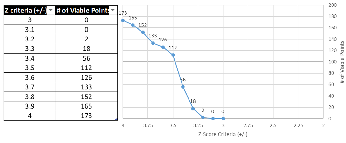
We analyze the sensitivity of potentially viable points to different z-score thresholds, under current settings. Figure 19 shows the number of viable parameter points as the z-score threshold is reduced. Note, however, that this set is a result of the +/-4 threshold setting for the Active Learning algorithm from the first run of the simulation. If the threshold condition were initially tighter (say +/-3 or +/-2,) we expect the resulting set of potentially viable points to be different. Figure 19 below represents a set of points from which fall within z=+/4 and z=+/-2 range.
A note on sensitivity of z-score thresholds:
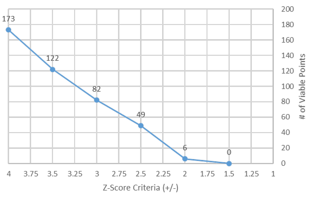
Another approach to a tighter fit (reduced z-score thresholds) between simulation output and empirical data in our simulation could be to consider a more selective subset of clinics used for history matching. E.g., dropping clinic 1273871 from consideration (where 0 visits result in a z-score between +/-4,) results in 82 points at z +/- 3 and points at z +/- 2. The sensitivity of the number of viable points to different z-score criteria under this exemplar restricted scenario is shown below in Figure 20.
A note on the stepwise tightening of viability constraints:
The aim of our paper is a methodological case study in model exploration techniques, and our approach represents the first step in a stepwise tightening towards identifying parameter value combinations where model output is potentially compatible with empirical data. The model exploration techniques we use to partition the parameter space into potentially viable and non-viable regions is methodologically similar to history matching as described in Holden et al. (2018), where non-viable regions are selectively removed in expensive simulators. Our stepwise tightening approach is driven by the goal of reducing computational costs compared to using standalone approaches like ABC.
References
ALTMAN, D. G., & Bland, J. M. (1994a). Diagnostic tests. 1: Sensitivity and specificity. British Medical Journal, 308(6943), 1552. [doi:10.1136/bmj.308.6943.1552]
ALTMAN, D. G., & Bland, J. M. (1994b). Statistics notes: Diagnostic tests 2: Predictive values. British Medical Journal, 309(6947), 102. [doi:10.1136/bmj.309.6947.102]
ANDRIANAKIS, I., Vernon, I. R., McCreesh, N., McKinley, T. J., Oakley, J. E., Nsubuga, R. N., Goldstein, M., & White, R. G. (2015). Bayesian history matching of complex infectious disease models using emulation: A tutorial and a case study on hiv in uganda. PLoS Computational Biology, 11(1). [doi:10.1371/journal.pcbi.1003968]
BAKER, E., Barbillon, P., Fadikar, A., Gramacy, R. B., Herbei, R., Higdon, D., Huang, J., Johnson, L. R., Mondal, A., Pires, B., & others. (2020). Stochastic simulators: An overview with opportunities. arXiv Preprint arXiv:2002.01321.
BELLMAN, R. (1961). Curse of Dimensionality. Adaptive Control Processes: A Guided Tour. Princeton, NJ: Princeton University Press.
BERGSTRA, J., & Bengio, Y. (2012). Random search for hyper-parameter optimization. Journal of Machine Learning Research, 13(Feb), 281–305.
BINOIS, M., Gramacy, R. B., & Ludkovski, M. (2018). Practical Heteroscedastic Gaussian Process Modeling for Large Simulation Experiments. Journal of Computational and Graphical Statistics, 27(4), 808–821. [doi:10.1080/10618600.2018.1458625]
CEVIK, M., Ergun, M. A., Stout, N. K., Trentham-Dietz, A., Craven, M., & Alagoz, O. (2016). Using active learning for speeding up calibration in simulation models. Medical Decision Making, 36(5), 581–593. [doi:10.1177/0272989x15611359]
COLLIER, N., & North, M. (2013). Parallel agent-based simulation with repast for high performance computing. Simulation, 89(10), 1215–1235. [doi:10.1177/0037549712462620]
COLLIER, N. T., Ozik, J., & Macal, C. M. (2015). Large-scale agent-based modeling with repast HPC: A case study in parallelizing an agent-based model. Proceedings of the Euro-Par 2015: Parallel Processing Workshops - Euro-Par 2015 International Workshops, Vienna, Austria, August 24-25, 2015, Revised Selected Papers, 454–465. https://doi.org/10.1007/978-3-319-27308-2_37 [doi:10.1007/978-3-319-27308-2_37]
CONSTANTINE, P. (2015). Active Subspaces: Emerging Ideas for Dimension Reduction in Parameter Studies. SIAM-Society for Industrial and Applied Mathematics. [doi:10.1137/1.9781611973860]
CRAIG, P. S., Goldstein, M., Seheult, A. H., & Smith, J. A. (1997). Pressure matching for hydrocarbon reservoirs: A case study in the use of bayes linear strategies for large computer experiments. Lecture Notes in Statistics book series (LNS, volume 121). Berlin Heidelberg: Springer, pp. 37–93. [doi:10.1007/978-1-4612-2290-3_2]
DAGUM, L., & Menon, R. (1998). OpenMP: An industry standard api for shared-memory programming. Computational Science & Engineering, IEEE, 5(1), 46–55. [doi:10.1109/99.660313]
EDMONDS, B., Le Page, C., Bithell, M., Chattoe-Brown, E., Grimm, V., Meyer, R., Montañola-Sales, C., Ormerod, P., Root, H., & Squazzoni, F. (2019). Different modelling purposes. Journal of Artificial Societies and Social Simulation, 22(3), 6: https://www.jasss.org/22/3/6.html. [doi:10.18564/jasss.3993]
EDWARDS, N. R., Cameron, D., & Rougier, J. (2011). Precalibrating an intermediate complexity climate model. Climate Dynamics, 37(7-8), 1469–1482. [doi:10.1007/s00382-010-0921-0]
FLÖTTERÖD, G., Bierlaire, M., & Nagel, K. (2011). Bayesian demand calibration for dynamic traffic simulations. Transportation Science, 45(4), 541–561.
FREETH, A., Pawlikowski, K., & McNickle, D. (2012). Pseudo-random number generators for massively parallel discrete-event simulation. University of Cantebury. http://hdl.handle.net/10092/9689.
GALLAGHER, S., Richardson, L. F., Ventura, S. L., & Eddy, W. F. (2018). SPEW: Synthetic populations and ecosystems of the world. Journal of Computational and Graphical Statistics, 1–12. [doi:10.1080/10618600.2018.1442342]
GARCIA, A. G. (2000). Orthogonal sampling formulas: A unified approach. SIAM Review, 42(3), 499–512. [doi:10.1137/s0036144599363497]
GARIBAY, L., Makelarski, J., & Lindau, S. (2014). South side population and vitality studies health study report. South Side Health; Vitality Studies, The University of Chicago.
HAN, G., Santner, T. J., & Rawlinson, J. J. (2009). Simultaneous determination of tuning and calibration parameters for computer experiments. Technometrics, 51(4), 464–474. [doi:10.1198/tech.2009.08126]
HARTIG, F., Calabrese, J. M., Reineking, B., Wiegand, T., & Huth, A. (2011). Statistical Inference for Stochastic Simulation Models – Theory and Application. Ecology Letters, 14(8), 816–827. [doi:10.1111/j.1461-0248.2011.01640.x]
HIGDON, D., Gattiker, J., Williams, B., & Rightley, M. (2008). Computer model calibration using high-dimensional output. Journal of the American Statistical Association, 103(482), 570–583. [doi:10.1198/016214507000000888]
HOLDEN, P. B., Edwards, N. R., Hensman, J., & Wilkinson, R. D. (2018). ABC for climate: Dealing with expensive simulators. Handbook of Approximate Bayesian Computation, 569–595.
JIN, R., Chen, W., & Sudjianto, A. (2002). On sequential sampling for global metamodeling in engineering design. ASME 2002 International Design Engineering Technical Conferences and Computers and Information in Engineering Conference, 539–548. [doi:10.1115/detc2002/dac-34092]
KALIGOTLA, C., Ozik, J., Collier, N., Macal, C. M., Lindau, S., Abramsohn, E., & Huang, E. (2018). MODELING an informat ion-based community health intervention on the south side of chicago. Proceedings of the 2018 Winter Simulation Conference. [doi:10.1109/wsc.2018.8632525]
KARYPIS, G., & Kumar, V. (1999). A fast and highly quality multilevel scheme for partitioning irregular graphs. SIAM Journal on Scientific Computing, 20(1), 359—–392. [doi:10.1137/s1064827595287997]
KENNEDY, M. C., & O’Hagan, A. (2001). Bayesian calibration of computer models. Journal of the Royal Statistical Society: Series B (Statistical Methodology), 63(3), 425–464. [doi:10.1111/1467-9868.00294]
LAMPERTI, F., Roventini, A., & Sani, A. (2018). Agent-based model calibration using machine learning surrogates. Journal of Economic Dynamics and Control, 90, 366–389. [doi:10.1016/j.jedc.2018.03.011]
LAROCHELLE, H., Erhan, D., Courville, A., Bergstra, J., & Bengio, Y. (2007). An empirical evaluation of deep architectures on problems with many factors of variation. Proceedings of the 24th International Conference on Machine Learning, 473–480. [doi:10.1145/1273496.1273556]
LETTIERI, N., Spagnuolo, C., & Vicidomini, L. (2015). 'Distributed Agent-Based Simulation and GIS: An Experiment with the Dynamics of Social Norms.' In S. Hunold, A. Costan, D. Giménez, A. Iosup, L. Ricci, M. E. Gómez Requena, V. Scarano, A. L. Varbanescu, S. L. Scott, S. Lankes, J. Weidendorfer, & M. Alexander (Eds.), Euro-Par 2015: Parallel Processing Workshops. Berlin Heidelberg: Springer, pp. 379–391.
LINDAU, S. T., Makelarski, J. A., Abramsohn, E. M., Beiser, D. G., Boyd, K., Chou, C., Giurcanu, M., Huang, E. S., Liao, C., Schumm, L. P., & others. (2019). CommunityRx: A real-world controlled clinical trial of a scalable, low-intensity community resource referral intervention. American Journal of Public Health, 109(4), 600–606. [doi:10.2105/ajph.2018.304905]
LINDAU, S. T., Makelarski, J., Abramsohn, E., Beiser, D. G., Escamilla, V., Jerome, J., Johnson, D., Kho, A. N., Lee, K. K., Long, T., & others. (2016). CommunityRx: A population health improvement innovation that connects clinics to communities. Health Affairs, 35(11), 2020–2029. [doi:10.1377/hlthaff.2016.0694]
LIPTON, Z. C., Elkan, C., & Narayanaswamy, B. (2014). Thresholding classifiers to maximize f1 score. arXiv Preprint arXiv:1402.1892.
MACAL, C. M., Collier, N. T., Ozik, J., Tatara, E. R., & Murphy, J. T. (2018). ChiSIM: An agent-based simulation model of social interactions in a large urban area. Proceedings of the 2018 Winter Simulation Conference. [doi:10.1109/wsc.2018.8632409]
MACAL, C. M., North, M. J., Collier, N., Dukic, V. M., Wegener, D. T., David, M. Z., Daum, R. S., Schumm, P., Evans, J. A., Wilder, J. R., Miller, L. G., Eells, S. J., & Lauderdale, D. S. (2014). Modeling the transmission of community-associated methicillin-resistant Staphylococcus aureus: A dynamic agent-based simulation. Journal of Translational Medicine, 12(1), 124. [doi:10.1186/1479-5876-12-124]
MAKELARSKI, J. A., Lindau, S. T., Fabbre, V. D., Grogan, C. M., Sadhu, E. M., Silverstein, J. C., Tran, T. T. T., Van Haitsma, M., Whitaker, E., & Johnson, D. (2013). Are your asset data as good as you think? Conducting a comprehensive census of built assets to improve urban population health. Journal of Urban Health, 90(4), 586–601. [doi:10.1007/s11524-012-9764-9]
OZIK, J., Collier, N., Wozniak, J. M., Macal, C. M., & An, G. (2018). Extreme-scale dynamic exploration of a distributed agent-based model with the emews framework. IEEE Transactions on Computational Social Systems, 4(3), 884–895. [doi:10.1109/tcss.2018.2859189]
OZIK, J., Collier, N., Wozniak, J. M., & Spagnuolo, C. (2016). From desktop to large-scale model exploration with Swift/T. Proc. Winter Simulation Conference. [doi:10.1109/wsc.2016.7822090]
PACE, W. D., Dickinson, L. M., & Staton, E. W. (2004). Seasonal variation in diagnoses and visits to family physicians. The Annals of Family Medicine, 2(5), 411–417. [doi:10.1370/afm.73]
REUILLON, R., Schmitt, C., De Aldama, R., & Mouret, J.-B. (2015). A new method to evaluate simulation models: The calibration profile (CP) algorithm. Journal of Artificial Societies and Social Simulation, 18(1), 12: https://www.jasss.org/18/1/12.html [doi:10.18564/jasss.2675]
RUTTER, C., Ozik, J., DeYoreo, M., & Collier, N. (2019). Microsimulation model calibration using incremental mixture approximate Bayesian computation. Annals of Applied Statistics, in Press. [doi:10.1214/19-aoas1279]
SETTLES, B. (2012). Active Learning. Synthesis Lectures on Artificial Intelligence and Machine Learning. Morgan & Claypool Publishers. [doi:10.2200/s00429ed1v01y201207aim018]
SKOLASKY, R. L., Green, A. F., Scharfstein, D., Boult, C., Reider, L., & Wegener, S. T. (2011). Psychometric properties of the patient activation measure among multimorbid older adults. Health Services Research, 46(2), 457–478. [doi:10.1111/j.1475-6773.2010.01210.x]
TANG, B. (1993). Orthogonal array-based latin hypercubes. Journal of the American Statistical Association, 88(424), 1392–1397. [doi:10.1080/01621459.1993.10476423]
WILLIAMSON, D., Goldstein, M., Allison, L., Blaker, A., Challenor, P., Jackson, L., & Yamazaki, K. (2013). History matching for exploring and reducing climate model parameter space using observations and a large perturbed physics ensemble. Climate Dynamics, 41(7-8), 1703–1729. [doi:10.1007/s00382-013-1896-4]
WOZNIAK, J. M., Armstrong, T. G., Wilde, M., Katz, D. S., Lusk, E., & Foster, I. T. (2013). Swift/T: Large-scale application composition via distributed-memory dataflow processing. Cluster, Cloud and Grid Computing (CCGrid), 2013 13th IEEE/ACM International Symposium on, 95–102. [doi:10.1109/ccgrid.2013.99]
WOZNIAK, J. M., Jain, R., Balaprakash, P., Ozik, J., Collier, N. T., Bauer, J., Xia, F., Brettin, T., Stevens, R., Mohd-Yusof, J., & others. (2018). Candle/supervisor: A workflow framework for machine learning applied to cancer research. BMC Bioinformatics, 19(18), 491. [doi:10.1186/s12859-018-2508-4]
XU, J. (2017). 'Model calibration.' In A. Tolk, J. Fowler, G. Shao, & E. Yücesan (Eds.), Advances in Modeling and Simulation: Seminal Research from 50 Years of Winter Simulation Conferences. Berlin Heidelberg: Springer, pp. 27–46.
XU, J., Vidyashankar, A., & Nielsen, M. K. (2014). Drug resistance or re-emergence? Simulating equine parasites. ACM Transactions on Modeling and Computer Simulation (TOMACS), 24(4), 1–23. [doi:10.1145/2627736]
XU, Z., Akella, R., & Zhang, Y. (2007). Incorporating diversity and density in active learning for relevance feedback. European Conference on Information Retrieval, 246–257. [doi:10.1007/978-3-540-71496-5_24]
YUAN, J., Ng, S. H., & Tsui, K. L. (2012). Calibration of stochastic computer models using stochastic approximation methods. IEEE Transactions on Automation Science and Engineering, 10(1), 171–186. [doi:10.1109/tase.2012.2199486]