
Introduction
Social archaeology focuses on the construction of the social space, the exploration of social processes in past societies; and on coming up with models, hypotheses and interpretations on how individuals or groups experience and influence their own societies, and how these constructed narratives of the past can or do influence modern societies. Likewise, the neighbouring discipline of computational archaeology focuses on the utilization of computational and computer-based methods for the study of behavioural evolution, allowing social scientists to model and carry out research in a formal and comprehensible way. Over the past two decades, the social and computational archaeology has utilized agent-based modeling (ABM)[1] for simulating past societies socio-ecological processes based on archaeological information and hypotheses (Axtell et al. 2002; Janssen 2009; Heckbert 2013; Cockburn et al. 2013). This is due to an ABMs’ ability to represent individuals or societies, and encompass uncertainty inherent in archaeological theories. In order to efficiently encapsulate human agency and quantitatively represent and explore specific properties and patterns of archaeological information, incorporating ideas from multiagent systems (MAS) research in ABMs can enhance agent sophistication, and contribute on the application of strategic principles for selecting among agent behaviours (Wellman 2016).
To this end, a recently developed ABM with autonomous, utility-based agents explores alternative hypotheses regarding the social organization of ancient societies, by incorporating different social organization paradigms and subsistence technologies ((Chliaoutakis & Chalkiadakis 2016). Specifically, it employs a “self-organization" social organization behaviour that allows the exploration of the historical social dynamics–i.e., the evolution of social relationships within the artificial agent community, considering a decentralized structural adaptation algorithm (Kota et al. 2009), while being grounded on archaeological information and evidence. In this work, we extend this ABM to simulate the artificial societies’ inter-settlement interactions, by developing a trading sub-model that is able to model the exchange and distribution of resources across artificial agent communities. In particular, in this trading sub-model, two well-known spatial interaction models are currently enabled, the XTENT (Renfrew & Level 1979) and Gravity (Huff 1964) model, to formulate the trading network across agent communities (while any other spatial interaction algorithm of choice can be potentially accommodated by our model). As such, our approach is able to provide insights on the social organization of the artificial society on a higher level than the original ABM; that is, it models and studies inter-settlement interactions, rather than solely intra-settlement ones.
As a case study, we utilize the ABM to explore hypotheses on settlement patterns, structure and potential trading organization of Minoan household agent communities (settlements), in the wider area of Knossos at the island of Crete (Greece), during the Bronze Age. The case study readily incorporates knowledge on archaeological sites locations and settlement types. Moreover, a conceptual natural disaster sub-model was also incorporated in the ABM, in an attempt to provide insights to whether the effects of the volcanic eruption of Thera (Santorini), ca. 1600 BCE, affected the trading network behaviour and set in motion the process that led to the breakdown of Minoan society (Chliaoutakis et al. 2018).
The main contributions of our work can be summarized as follows:
- We provide a novel trading model that readily incorporates spatial interaction paradigms to simulate trade among self-organized communities of autonomous utility-based agents.
- We incorporate a natural disaster sub-model into the ABM, to provide insights on how a natural disaster scenario could have affected the trading network behaviour and further the agent communities organization structure.
- We utilize graph theory to analyze the trading network, and thus interpret simulation results in terms of the network’s potential centralization, clustering behaviour or potential settlement organization during the whole simulation period.
- Our systematic study of the dynamic trading network provides support to certain archaeological hypotheses related to the specific period and modeling area of study.
- We exploit simulation results to derive intuitions regarding the appropriateness of different spatial inter- action models.
Specifically, our simulation results show that modeling a trading network that takes into account mainly the settlements’ “importance" (e.g. in terms of population size or lifetime) rather than solely the distance between settlement locations, can produce settlement patterns similar to the one that exist in archaeological record. However, this is most appropriate when the settlements’ importance is known or can be derived based on archaeological evidence, thus allowing such a trading model to better capture the trend in settlement numbers that exist in the archaeological record. By contrast, when settlements’ importance is not known, or cannot be properly modeled, then a trading network model should favour the distance between settlements rather than their importance.
Overall, the evolution of the values of the graph-theoretic indices characterizing our simulations’ network (i.e. clustering coefficient, in-degree and out-degree centrality) indicate that the Minoan’s trading network (at the modeling area) was affected by the Theran volcanic eruption. Specifically, it appears that the trading network in the Late Minoan (LM) period becomes clearly denser, while it seems that there exist only a few “important centres" at the time, which is in line with the archaeological record. Moreover, it appears that the trading net- work’s structure and interaction patterns are to an extent reversed after the Theran eruption, when compared to those in effect in earlier periods.
The rest of this paper is structured as follows: Section 2 provides a review of existing examples of archaeological ABMs in the literature. In Section 3 we provide a concise overview of the ABM, by describing its environmental representation; the agents and their interactions; and the agents social organization paradigms. Section 4 presents the theoretical background of the modeling process that was followed for developing the trading net- work across settlements, based on both the XTENT and Gravity spatial interaction models. There, we also introduce several concepts from network and graph theory required for the analysis of the resulting trading network. Section 5 then presents our specific case study of early Minoan societies located at the wider central area of Knossos in the island of Crete. In addition, we record the empirical evaluation of the various trading models, in terms of potential settlement centralization and organization emerged during the Minoan period, by first detailing the simulation parameters for the various scenarios considered, and then analysing the obtained results. Finally, Section 6 concludes this work, and discusses simulation results and future research directions.
Background and Related Work
Social archaelogy seeks to understand the social organization of past societies at many different points in time (Renfrew & Bahn 2012). There is a great number of questions that may arise regarding the nature and internal organization of the society under study. For instance, are the main social units, individuals or groups, participate on a more-or-less equal basis, or do prominent differences in status or rank within the society (or perhaps even different social classes) exist? Answering these questions turns out to be harder when exploring prehistoric communities rather than later ones, as written records in early societies are scant. Surely, there are many methods for acquiring information regarding the internal social organization of an early society. Beyond field survey — which aims to discover mainly a presumed settlements hierarchy — one can make use of settlement pattern information, written records, oral tradition and approaches from ethno-archaeology (Renfrew & Bahn 2012). Clearly, the variety of methods used and the inherent uncertainty of the domain gives rise to a rich space of hypotheses for any given question regarding the social organization of early societies.
As such, the past few decades has seen archaeology taking an increasing interest in ABM (Doran et al. 1994; Dean et al. 2000; Axtell et al. 2002; Janssen 2009; Heckbert 2013; Cockburn et al. 2013; Crabtree et al. 2017). Its emerging popularity is due to the ABM’s ability to represent individuals and societies, and to encompass uncertainty inherent in archaeological theories. The unpredictability of interaction patterns within a simulated agent society, along with the strong possibility of emergent behaviour, can assist archaeology researchers to gain new insights into existing theories.
For example, a relatively recent ABM for understanding how prehistoric societies adapted to the American southwest landscape of their era is presented by Janssen (2010). That ABM could explore to some extent how various assumptions concerning social processes affect the population aggregation and size, and the dispersion of settlements. In that model, interactions (like the sharing of resources among the agents, or the exchange of resources among their settlements) are largely determined by rules that are built in the system. However, results suggest the temporal and spatial population dynamics are affected by many assumptions of the model; resource dynamics affect the long-term population levels, whereas climate variability affects the short-term aggregation levels of the prehistoric populations in American Southwest.
Likewise, Cockburn et al. (2013) developed an agent-based simulation of specialization in resource production, and a system of barter allowing exchange of specialized products between household agents, in Pueblo societies existing between 600–1300 CE in southwestern Colorado with the ultimate goal of examining their effects in these middle-range Neolithic societies. Much of the dynamism of the simulation is provided by annual and spatially specific estimates of potential maize production on this landscape (Kohler 2012). Agents are responsible for gathering and exchanging resources with other agents. In the case that agents cannot obtain all the resources they need on their own, they are allowed to exchange with other agents. Moreover, if an agent is not performing well at its present location, it will move to a more suitable location in the study area, by evaluating resource productivity of prospective areas. When an agent has excess storage of a resource, it will let other neighbouring agents know; and if they have higher production costs for these resources, they will predict that the agent will be able to help them meet any shortfall for this resource in the upcoming year. Although the authors are less concerned about the realism of some of the assumptions that are hard-coded in their model, they conclude that adding social influence to their reference system with economic specialization leads to a population that is not necessarily larger in size, but one that is more specialized.
Another recent example of a simulation model integrating cellular automata and a network model of the ancient Maya social-ecological system, is MayaSim (Heckbert 2013). The purpose of the model is to better understand the complex dynamics of social-ecological systems, and to test quantitative indicators of resilience as predictors of system sustainability or decline. Agents representing Maya settlements (rather than households), develop and expand within a landscape that changes under climate variation and anthropogenic pressure. Agents are utility-based in the sense that they estimate the utility of the various actions at hand. However, they choose actions whose utility has reached some thresholds that are in fact hard-coded by the modeller. Moreover, their utility function is affected by agent resource exchange that occur between settlement agents, since they are connected via a network of links that represent trade routes. The model was able to reproduce spatial patterns and timelines somewhat analogous to that of the ancient Maya, although this proof-of-concept stage model requires refinement and further archaeological data for better calibrations.
By contrast, Chliaoutakis & Chalkiadakis (2016) try to assess the influence of different social organization behaviours on population growth with respect to their geographic context and available archaeological evidence. Specifically, the ABM’s case study is regarding the Minoan civilization, in the “Malia" area at the island of Crete, Greece, during the Bronze Age period. The ABM incorporates several social organization paradigms, giving emphasis to a self-organization social behaviour, where household agents within a settlement continuously reassess their relations with others. An alternative “evolutionary" self-organization social behaviour was also introduced by the same authors, driven by the interactions of strategic agents operating within a given agent community (Chliaoutakis & Chalkiadakis 2017). They Incorporated evolutionary game-theory into the agents social organization process, by simulating repeated “stage games" played by any pair of agents within an agent com- munity, in order to assess the effects these interactions have on population viability and strategic behaviours that may emerge in the long-term. When agents adopt an “egalitarian-like" social organization paradigm, the emerging development of many “small-size" settlements seems to be the way for survival over time. When the self-organization social paradigm was adopted for determining household agents relations, a “heterarchical" social structure emerges, rather than a clear "hierarchical" one evident in later periods.[2] Simulation results demonstrated that self-organized agent societies appear to be giving rise to larger settlements during their evolution, maintaining larger population sizes than the "egalitarian" distributive one. This fact, is in line with archaeological evidence for larger settlements (towns and palaces) eventually coming to existence during the Middle/Late Minoan period, where a more varied social structure is now suggested (Driessen & Langohr 2014).
As a final note, and to the best of our knowledge, the only archaeology-related ABM that utilizes a spatial inter- action model, is that of Graham (2006) . The ABM simulates movement of travellers (agents) between settlement locations known through archaeological field survey in specific regions of Central Greece during the Geometric period and Central Italy during Protohistory. The author utilizes an entropy-maximizing model, that is, the Gravity spatial interaction model, in order to ultimately rank the settlements by the number of times they emerged as most “important" in the various metrics of the travellers network. Agents in the ABM are only able to travel to settlements around their neighbourhood and only to the most attractive site out of three potential destinations. Although the factual description of the ABM is missing, since the author argues that the mathematics in the ABM are not the most important consideration, but rather the description of how the agents interact, some indicative results are presented and discussed.[3]
A utility-based ABM
Against the background presented above, we present here an ABM that serves the following purposes: (a) it can be employed for the study of practically any society of choice in a specific geographic context, and can easily incorporate and assess hypotheses regarding socio-economic processes proposed by archaeologists; and (b) it showcases how MAS-originating concepts, techniques, and algorithms can be employed in archaeology-related ABMs. Unlike most existing ABM approaches in archaeology, which employ a simple reflex agent architecture, the ABM here employs utility-based agents that act autonomously towards utility maximization, and can build and maintain complex social structures.[4] Indeed, using ABMs that were built on knowledge derived from archaeological research, but do not attempt to fit their results to a specific material culture, allows for the emergence of dynamics for different types of societies in different types of landscapes. This aids the generation of new hypotheses, as well as the transfer and re-use of knowledge beyond a specific case study.
In this work, we adopt and build on top of the work of Chliaoutakis & Chalkiadakis (2019). Agents correspond to households, each containing up to a maximum number of individuals (people).[5] Each household agent resides in a cell within the environmental grid, with the cell potentially shared by a number of agents. Adjacent cells occupied by agents make up a settlement—and there is at least one occupied cell in a settlement. Households are utility-based autonomous agents who can settle (or occasionally resettle) and cultivate in a specific environmental location. They also possess an explicit representation of the environmental grid, and use this to choose the best available migration location they can move to within a pre-specified radius, to improve their utility.
The total number of agents in the system changes over time, as individuals belonging to household agents born or die. Agent procreation ability, determining the annual levels of births of household inhabitants, is based on the amount of energy consumed by a household agent \(x\) during the year. This in turn depends on the resources harvested, that is, the agent’s utility \(U_x\), which is a function of population size and available resources at a given location, as we explain below. When household inhabitants exceed a critical number, new households (agent offsprings) are created; and when the agent overall utility levels are not high enough to sustain its people, the agent considers migrating to prevent individuals from dying.
Specifically, at every time step, agent \(x\) picks the best action \(b'\) in the set of actions \(Actions_x\) at its disposal:
| $$b' = argmax_{b \in Actions_x} {U_x(b)}$$ | (1) |
The main preoccupation of the agents is to stay alive by acquiring and consuming resources. If an agent fails to acquire enough energy it will eventually die out, since it will stop procreating. Acquiring energy is the only inbuilt goal of the agents. Currently, the only action available for agents to acquire energy is via harvesting the lands. This can be done (a) either at the agent’s current location (via employing the cultivation action); or (b) at some other location to which the agent migrates (migration action). Therefore, since there are only two actions to consider, the (expected) utility \(U_x\) of the agent \(x\) can be simply described as follows (assuming the agent cultivates n environmental cells):
| $$U_x{\rm =} \max \lbrace \sum^n_{{k=1}}{R_k}, U^\prime_x \rbrace$$ | (2) |
Now, agents in the model are able to employ several social organization paradigms, that is, resource distribution schemes, such as:[7]
- independent, where agents acquire and consume resources independently
- egalitarian-like, where acquired resources are pooled each year and distributed equally among the agents
- self-organized, where agents autonomously re-arrange their relations, and hence the underlying "social network structure" describing these relations, without any external control
- hierarchical, where agents distribute resources based on "static" relations, following the same rules as those governing the self-organized behaviour but without changing any relation during their evolution
Both in the "self-organized" and "hierarchical" social organization paradigms, agents relations determine the way resources are ultimately distributed among them.
The self-organization algorithm has two main stages: the task execution and re-allocation mechanism, by which it is decided which agents will receive (energy) resources from others to cover their needs, based on their relations; and the re-organization (decentralized structural adaptation) one, used for re-evaluating and potentially altering their relations at every time step. The evaluation that is performed during the re-organization stage is based on the relative difference of the overall utility "surplus" exchanged between a pair of agents, in case the relation had been different than the current one. Specifically, any interaction between a pair of household agents within a settlement, takes place based on the following relation types: acquaintance, peer or authority (superior - subordinate) related agents, where these relations give rise to a social structure reflecting the flow of resources during exchanges among the agents. The authority relation depicts "superior status" of an agent \(x\) over the subordinate agent \(y\) in the context of their social organization, reflecting that higher amount of resources flow from \(x\) to \(y\) during exchanges than those flowing in the opposite direction; the peer relation holds between agents who are considered more-or-less equal in status (i.e. flows involve resource transfers of almost equal amounts in both directions); while acquainted agents are aware of each other’s presence, but have no interaction. Agents use the information about all their past and current year allocations to re-evaluate their relations with others. Thus, agents may improve their performance as a "group" (vitality of the settlement) by modifying the social structure through changes to their relations (re-organization) continuously over time (Chliaoutakis & Chalkiadakis 2016).
Modeling Trade Across Settlements
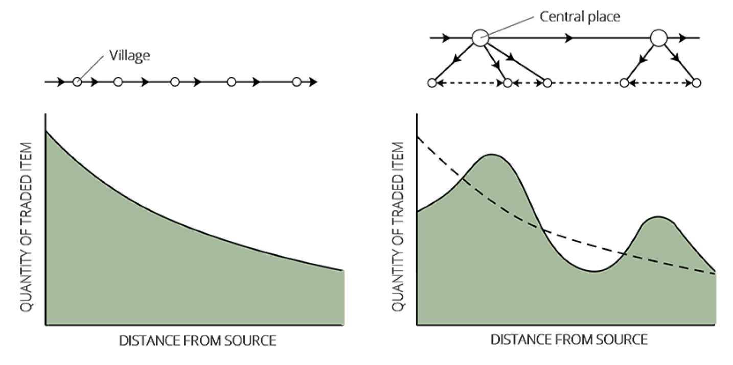
In this work we extend the intra-settlement exchange of resources (household level) to inter-settlement inter- actions (settlement level). Certainly, in the absence of written records it is not easy to determine what were the mechanisms of trade, or what was the nature of the exchange relationship. However, several formal techniques are available for the study of trade, such as the development of a distribution map for finds or materials, within a specific geographic area (Renfrew & Bahn 2012). Considering such distribution maps, pondered by fall-off analysis, the quantity of a traded material usually declines as the distance from the source increases.
For instance, let us consider a "down-the-line" trading system (Renfrew & Bahn 2012). If one site, e.g. village, receives its supplies of a raw material down a linear trading network from its neighbour site up the line, it may retain a given proportion of the material for its own use, and trade the remainder to its neighbour site down the line. If each village does the same, an exponential fall-off curve will result, as illustrated in Figure 1 . In some cases, however, there are regularities in the way in which the decrease occurs, and this pattern can inform us about the mechanism by which a material reached its destination. As an example, a different distribution system, through major and minor sites, would produce a different fall-off pattern, in particular, a multi-modal fall-off curve, since lower-order settlements tend to exchange with higher-order centres, even if the latter lies further from the source than an accessible lower-order settlement (Figure 1). We note at this point that in the rest of this paper we shall use the term "settlement" to refer to any site category, such as village, town, etc.
A possible solution to conceptualize exchange and distribution of resources (flows) between settlements, relies on using a spatial interaction model (Renfrew & Bahn 2012; Rodrigue et al. 2017). The basic assumption regarding spatial interaction models is that flows are a function of the attributes \(W_i\) of the origin location \(i\), and the attributes \(W_j\) of the destination location \(j\) and the "friction" of distance \(D_{i,j}\) between the concerned origin and destination locations. The general formulation of the spatial interaction model is as follows (Rodrigue et al. 2017):
| $$I_{i,j}=f(W_i,W_j,D_{i,j})$$ | (3) |
In our work here, \(I_{i,j}\) represents a measure of “attractiveness" corresponding to the interaction probability or probability of trade between settlements \(i\) and \(j\). \(D_{i,j}\) is the distance between the settlement locations.[8] Variables \(W_i\) or \(W_j\) are used to express a measure of "importance" for settlement \(i\) and \(j\), respectively. Attributes often used to express such variables are socio-economic in nature, such as population or gross domestic product in modern societies.
Since we are calculating the settlements’ interaction probability at any given time-step t during the simulation, we consider the following attributes:
- \(P_{j,t}\) defined as the ratio of the population of settlement \(j\) (i.e., the total number of its household’s inhabitants) with respect to the total population at time \(t\), and
- \(K_{j,t}\) defined as the ratio of the number of time steps that settlement \(j\) has existed so far up to \(t\).
Then, at any given time-step \(t\), we define the weight of importance \(W_{j,t}\) of a settlement location \(j\) as follows:
| $$W_{j,t} = \sqrt{P_{j,t}} \cdot \sqrt{K_{j,t}}$$ | (4) |
For example, assume that at time-step \(t\)= 1000 \(S_i\) settlements exist in the ABM environmental area, where \(i = {1, 2}\) and the total population is 8000 inhabitants; and assume that \(S_1\) has a population of 2880 inhabitants and a lifetime of 810 years while \(S_2\) has a population of 5120 inhabitants and a lifetime of 360 years up to current (annual) time-step \(t\). Then \(W_{i,t}\) is calculated as follows:
| $$W_{1,1000} = \sqrt{P_{1,1000}} \cdot \sqrt{K_{1,1000}} = \sqrt{\frac{2880}{8000}} \cdot \sqrt{\frac{810}{1000}} = 0.6 \cdot 0.9 = 0.54 \\ W_{2,1000} = \sqrt{P_{2,1000}} \cdot \sqrt{K_{2,1000}} = \sqrt{\frac{5120}{8000}} \cdot \sqrt{\frac{360}{1000}} = 0.8 \cdot 0.6 = 0.48$$ |
Thus, settlement \(S_1\) has a higher weight (of importance) than settlement \(S_2\), even though \(S_2\) has an almost double population size than \(S_1\), due to the higher lifetime of \(S_1\) during the simulation.
Now, past societies of the first farmers in different parts of the world, may be generally described as independent sedentary and relatively egalitarian communities without any strongly centralized organization (Renfrew & Bahn 2012). Following the development of farming, in many cases, the farming economy underwent a process of intensification, associated with developing exchange. Given this, we make the following assumption: at any given time-step \(t\), each (household) agent within a settlement i is socially contracted as a community member to give away a portion of its stored surplus \(ps\) (e.g. 20% or 80%) to be communally pooled as the corresponding settlement trading resources \(N_{i,t}\) and be traded away by the settlement later on. We note that the percentage of surplus resources that an agent is able to give away is user-defined in the ABM.
For instance, if at time \(t\) = 1400, settlement \(S_{53}\) has \(a_i\) households (agents), where \(i = {1, 2 ,3}\), and each agent has \(st_i\) surplus resources in its storage, e.g., \(st_1\) = 100, \(st_2\) = 200, \(st_3\) = 50, while the user-defined percentage of stored surplus to be given away is \(ps\) = 20%, then the settlement’s overall trading resources unit \(N_{53,1400}\) are calculated as follows:
| $$N_{53,1400} = ps \cdot \sum_{i=1}^{3} st_i = 0.2 \cdot (100 + 200 + 50) = 70$$ |
Then, settlement \(i\) can ultimately trade and exchange resources \(E_{i,j,t}\) with settlement \(j\) at time-step \(t\), by distributing its trading resources \(N_{i,t}\) based on its interaction probability \(I_{i,j,t}\), as follows:
| $$E_{i,j,t} = \frac{I_{i,j,t} \cdot N_{i,t}} {\sum_{j=1}^{n} I_{i,j,t}}$$ | (5) |
To give some intuition on the calculation of \(E_{i,j,t}\) let us provide another example; however, in order to not overload notation, we are dropping the \(t\) index, when this is not required. Thus, if we consider a set of potentially interacting settlements \(S_i\) where \(i = \{1,2,3,4,5\}\) and \(I_{i,j}\) is provided by some spatial interaction model (e.g., the XTENT or Gravity used in this work), so that \(I_{1,2} = 0.2\), \(I_{1,3} = 0.6\), \(I_{1,4} = 0.8\), \(I_{1,5} = 0.4\) then settlement \(S_1\) will distribute a portion of its trading resources, e.g., \(N_1\) = 200 (in kg) to settlement \(S_2\), as follows:
| $$E_{1,2} = \frac{I_{1,2} \cdot N_1} {\sum_{j=1}^{5} I_{1,j}} = \frac{0.2 \cdot 200}{0.2 + 0.6 + 0.8 + 0.4} = 20$$ |
As such, \(S_1\) will give away 10% of its overall trading resources to settlement \(S_2\), 30% to settlement \(S_3\), 40% to settlement \(S_4\) and 20% to settlement \(S_5\)— in the event that trade occurs with the corresponding probabilities. Similarly, when the trading process is over, settlement \(i\) will proportionally distribute the “public good" payoff among its household agents, based on their number of inhabitants.
We elaborate on the XTENT and Gravity spatial interaction models immediately below.
The XTENT model
The XTENT model asserts some relationship of settlement size and distance, whereby the larger dominates the smaller if the distance between them is sufficiently small, whereas the smaller retains autonomy if that distance is large enough (Renfrew & Level 1979). Thus, it assumes that a large centre will dominate a small one if they are close together; in political terms the smaller site has no independent or autonomous existence. This approach overcomes the limitation of the Thiessen polygons method, where territories are assigned irrespective of the size of the settlement, and where there are no dominant or subordinate settlements, allowing a simple approximation of the political reality and a hypothetical political map to be constructed (Renfrew & Bahn 2012).
In our ABM, the “attractiveness" determining the level of trading interaction of settlement \(i\) (origin location) with settlement \(j\) (destination location) that relies on the XTENT formula, is proportional to the importance of the destination location and declines linearly with their distance, as follows:
| $$I_{i,j} = W_j / D_{i,j}^\lambda$$ | (6) |
Given the \(I_{i,j}\)’s, one can provide visualization intuitions about settlement main trading territories by coloring each “cell" in the modeling area with the same color of the settlement to which it is mostly attracted to (see Figure 12 in Appendix).
The Gravity model
The Gravity model is the most common formulation of the spatial interaction method (Rodrigue et al. 2017). It is named as such because it uses a similar formulation as the Newton’s law of gravity. The "attractiveness" between the locations of origin \(i\) and destination \(j\) that relies on the Gravity model is proportional to the importance of the destination location and inversely proportional to their respective distance (Huff 1964):
| $$I_{i,j} = W_j / D_{i,j}^\lambda$$ | (7) |
Likewise, one would of course need to experiment with \(\lambda\) in order to efficiently reflect the required (growing) effect that distance have to the trading probability between settlements \(i\) and \(j\). In our simulations experiments and same as with the XTENT model, \(I_{i,j}\) also scaled to [0;1] (min-max normalization).
An example of settlement “trading" territories relying on the Gravity model is provided in Appendix A, Figure 13, by assuming the same settlement locations as in the previous example (cf. Figure 12, Appendix A) as destination locations, and origin locations to be any landscape cell in the modeling area.
Discussion on the spatial interaction models used
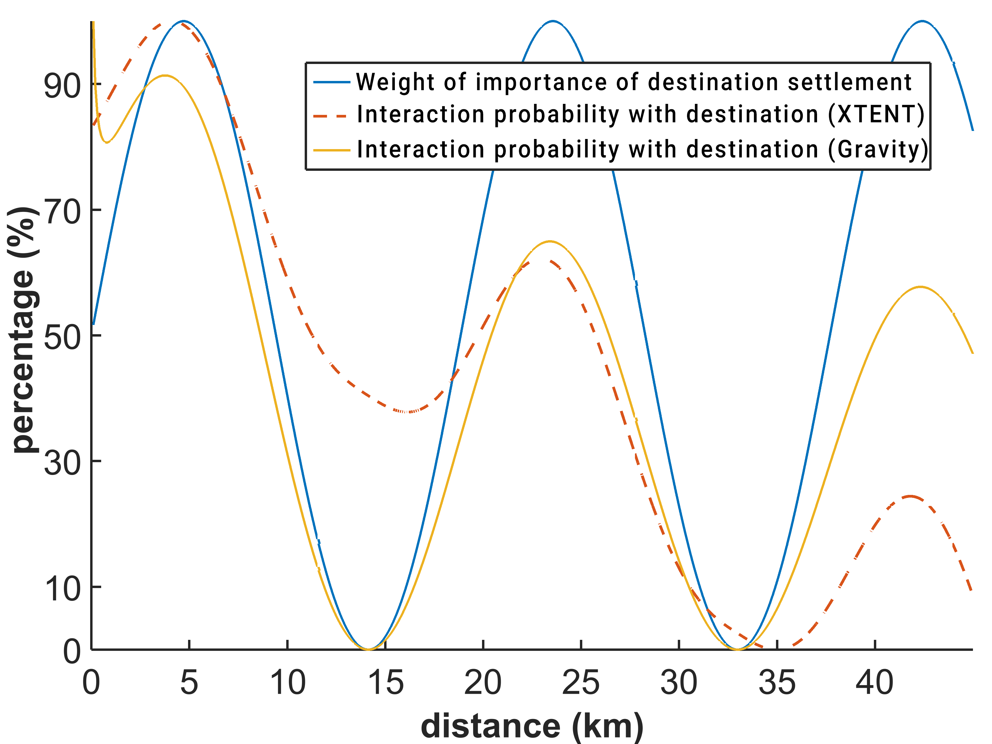
In the simulation scenarios described later on, we consider two different views on the trading probability between settlements; one favouring the distance between settlements rather than its importance, relying on the XTENT model with \(\beta=1.5\) and \(m=0.005\) (Equation 6), and another favouring the importance of settlement locations rather than the distance between them, enabled by the Gravity model with \(\lambda=0.2\) (Equation 7). We will observe these models’ effect on settlement organization and distribution patterns in our simulation results.
The aim of assigning the specific values of \(\beta\) and \(m\) for the XTENT model, and of \(\lambda\) for the Gravity model, is to adequately model the required trade-off between settlements distance and importance for the specific case study’s geographic area described later on (maximum distance of about 40 km). To provide an intuition on the two different views on the trading probability between settlements, let us assume that the probability distribution of “importance" for a potential destination settlement is as illustrated in Figure 2 (the blue dashed sinusoidal curve). The corresponding probability distribution of interaction of an origin settlement with the respective destination location is then depicted with the red and yellow curve, considering the XTENT and Gravity models, respectively. As shown in Figure 2, the distance between the origin and destination settlements has a greater role when the XTENT method is employed, while it has a lesser impact when the Gravity model is in use.
Graph theory for trading network analysis
In our ABM, settlements interact with several other settlements, formulating a different trading network at every given time-step during the simulation, based on the enabled trading scheme (XTENT or Gravity model). What we need to explore in such a dynamic trading network of settlements, is whether and to what degree some settlements are more important or central than others, based on their trading interactions; and whether settlements tend to create groups characterised by a relatively high density of trading interactions. Thus, in order to better understand and provide insights on the consequence of patterns of interaction between settlements, we adopt in our work some of the main approaches that network and graph theory has developed. We describe these below.
To begin with, a trading network can naturally be represented by a graph. A graph consists of a set of points and a set of edges or ties connecting pairs of points. In our case, each settlement location in the trading network corresponds to a point in the graph and each trading interaction (link) corresponds to an edge that connects a pair of settlement locations.
A fundamental measurement concept for the analysis of network graphs is centrality, that can highlight important information about the network organization and its structure (Freeman 1979). Centrality index describe point locations in terms of how close they are to the “centre" of the network activity. Thus, settlements who have more interaction ties (edges) to other settlements may be in advantaged positions. Because they have many interaction ties, they may have access to more of the exchanged resources over the network as a whole, and hence are less dependent on other settlements (Hanneman & Riddle 2005).
Whenever two settlements trade, they are directly connected by an edge, and thus, they are adjacent. The number of other settlements to which a given settlement is adjacent is called the degree of that settlement. A simple and effective measure of a settlement’s centrality is its degree. Since resources can be exchanged in a single edge direction towards another settlement, the temporal trading network of the ABM is represented as a “directed" graph and it is important to distinguish centrality based on in-degree, from centrality based on out-degree. If settlements receive many interaction ties, they can be described as prominent, or having high prestige, since many other settlements seek to direct resources to them, and this may indicate their importance (Hanneman & Riddle 2005). Settlements with high out-degree centrality are able to distribute resources to many other settlements, or make many other settlements aware of their resource exchange potential, thus being more influential than settlements with low out-degree centrality; although it might matter to which settlement they are distributing resources, this measure does not take that into account (Hanneman & Riddle 2005).
Let us now assume that a potential trading network is formulated with \(n\) number of settlements \(S_j\) (network nodes), at a specific time-step during the simulation in our ABM. This snapshot of the trading network can be represented as a directed graph, where numerous trading interactions occur between settlements. The in- degree or out-degree centrality index \(C_D(S_j)\) is the number of incoming or outgoing trading edges, respectively, for a settlement \(S_j\) (Freeman 1979):
| $$C_D(S_j) = \sum_{i=1}^{n} tr(S_i, S_j)$$ | (8) |
| $${C_D}^\prime(S_j) = \frac{C_D(S_j)}{n-1}$$ | (9) |
The effect of network size has been removed by normalizing with \(\max{C_D(S_j) = n - 1}\), since any given settlement \(S_j\) can at most be adjacent to \(n - 1\) other settlements in the trading network graph. Overall, the degree of a settlement point can be viewed as an index of its potential trading activity.
Another view of settlement point centrality, within a “directed" network graph, is based on the frequency with which a settlement \(S_k\) falls between pairs of other settlements on the shortest or “geodesic" paths connecting them, defined as the relative betweenness centrality index (White & Borgatti 1994):
| $${C_B}^\prime(S_k) = \frac{\sum_{i}^{n}\sum_{j}^{n} b_{i,j}(S_k)}{(n_I-1)(n_O-1)-(n_S-1)}, \\ \qquad b_{i,j}(S_k) = \frac{g_{i,j}(S_k)}{g_{i,j}}, \\ \qquad i \neq j \neq k$$ | (10) |
Now, when centrality is applied to the whole trading network graph, such a measure should index the degree to which the centrality of the most central settlement exceeds the centrality of all other settlements, and it is expressed as a ratio of that excess to its maximum possible value for the network graph containing the observed number of settlement points (Freeman 1979). Thus, the relative degree graph centrality index varies between 0 and 1, and is defined as follows:
| $${C_D}^\prime = \frac{\sum_{i=1}^{n} [{C_D}^\prime(S^*) - {C_D}^\prime(S_i)]}{\max\sum_{i=1}^{n}[{C_D}^\prime(S^*) - {C_D}^\prime(S_i)]}$$ | (11) |
Similarly, the relative betweenness graph centrality index varies between 0 and 1, and is defined as follows:
| $${C_B}^\prime = \frac{\sum_{i=1}^{n} [{C_B}^\prime(S^*) - {C_B}^\prime(S_i)]}{\max\sum_{i=1}^{n}[{C_B}^\prime(S^*) - {C_B}^\prime(S_i)]}$$ | (12) |
Then, high relative in-degree or out-degree graph centrality means that there are few settlements of high importance, or highly influential settlements respectively, in the trading network (and thus the most prominent or influential settlement in the network really “stands out”, making the value of the numerator in Equation 11 go up). On the other hand, low relative in-degree or out-degree graph centrality means that there are many settlements with a similar level of influence or importance. Accordingly, high relative betweenness graph centrality means that there are few settlements with high potential for control in the trading network, while low relative betweenness graph centrality means that there are many settlements that exhibit a similar potential for control in the trading network.
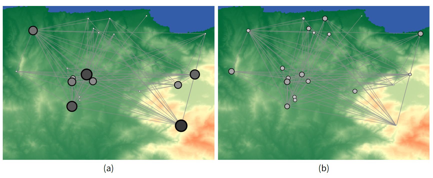
To provide visualization intuitions on the relative network graph centrality (Freeman 1979) we present a snapshot of the trading network developed during a random simulation run. In the example of Figure 3, each settlement node in the trading network is depicted with a circle, where its size and color represents its relative centrality value [0; 1], with white color corresponding to the minimum value (0) and black color corresponding to the maximum centrality value (1). Figure 3a illustrates a trading network of settlements with high relative graph centrality, while the one in Figure 3b shows the same network but with low relative graph centrality.
Besides the above relative graph centrality indices that will be used to evaluate the settlement trading network structural evolution, the degree to which settlements in the network graph tend to cluster together is also examined in our work, by calculating the network’s average clustering coefficient (Watts & Strogatz 1998):
| $$\tilde{C} = \frac{1}{n}\sum_{i=1}^{n} C_i$$ | (13) |
Case study: the Minoan Society in Central Crete, Greece
Several ancient civilizations existed in the Aegean Sea during the Bronze Age, with the island of Crete being associated with the "Minoan" civilization, which came to dominate the islands and the shorelines of the Aegean Sea. A significant shih in the early Minoans human existence and lifestyle was brought when crop farming was first developed. Previous reliance on a nomadic hunter-gatherer way of subsistence, was in time replaced by reliance on the produce of cultivated lands (Hamilakis 1996). These developments are assumed to have had great impact on the growth of settlements, encouraging the concentration of local population.
There is not enough information about what kind of relationships existed between the Minoans or how this ancient civilization was organized before the "Post-palatial" (Late Minoan) period. The sophistication of the Minoan culture and its trading capacity is evidenced by the presence of writing (mostly found on various types of administrative clay tablets). The content of the Minoan texts that have been unearthed is predominantly economic (inventories of goods or resources) and religious. Scholars argue that even if relations among (and possibly within) the various towns and cities continued to be contentious and competitive, a common architectural language was beginning to emerge (McEnroe 2010). This new architectural language marks the beginning of a specifically Minoan identity, which defines a clear indication that each household was not a self-sufficient, totally independent production unit, but that it was involved in exchange. Moreover, for the later Neolithic and Early Bronze Age, stylistic and petrographic analyses suggest a low-volume circulation of ceramic vessels, compatible with “gift exchange" economies, over short and long distances between different communities within and occasionally beyond the island (Tomkins & Schoep 2010). This evidence allows us to conceivably model such relations as resource exchanges.
We note, however, that we do not intend to generally reduce human relations to exchange, as if human ties to society can be imagined in the same terms as a business deal (Graeber 2011). Nevertheless, even Aristotle was speculating along similar lines in his treatise on Politics. At first, he suggested, families or households must have produced everything they needed for themselves. Gradually, some would presumably have specialized, some growing corn, others making wine, swapping or trading one for the other (Barnes et al. 2014; Graeber 2011). Therefore, although we do not have a clear picture of how human relations (interactions) were actually formed in prehistoric time periods, we need to have a conceivable conceptual model in mind, and that is done with the simplest possible way: to model trading among them as an exchange of resources—thus, giving us the ability to encode the conceptual model as an ABM encompassing various spatial interaction models for the resource exchange process, enabling us to explore a range of the its corresponding trading network structure in turn.
In addition, archaeologists argue that Minoan palaces are considered to be one of the central factors in bringing about social transformation in the Minoan civilization (Cherry 1986). In their view, the construction of Minoan palaces came about through a socio-political "quantum leap" from Chiefdom to State. This leap involved also the introduction of writing, the first centrally organized religion (the peak sanctuaries), and the development of social hierarchy and interacting social networks. Moreover, the size of such “grand" public structures at several sites requires both a considerable population and a social cohesion, and it can reasonably be assumed that there were different levels of importance, i.e. a hierarchy of sites (Driessen 2002).
Furthermore, a series of changes in the Aegean, and in particular in Cretan Bronze Age society, were triggered by the ca. 1600 BCE Santorini eruption (Driessen 2019). These changes would have caused the breakdown of the Minoan system over the course of a few generations, during 15th c. BCE. Archaeologists hypothesize that the eruption would have initially caused major problems in food production and distribution, undermining central authority and leading to a process of decentralization; this fragmentation would then have led incrementally to internal conflict. Despite the many destructions and abandonments documented, Minoan culture survived.
Starting from the above archaeological information about the Minoan society, we shall try to assess the resulting trading network structure over time and its effect on the Minoan society social organization at the community level, providing insights on settlement clustering and organization during the Bronze Age.
Model environment
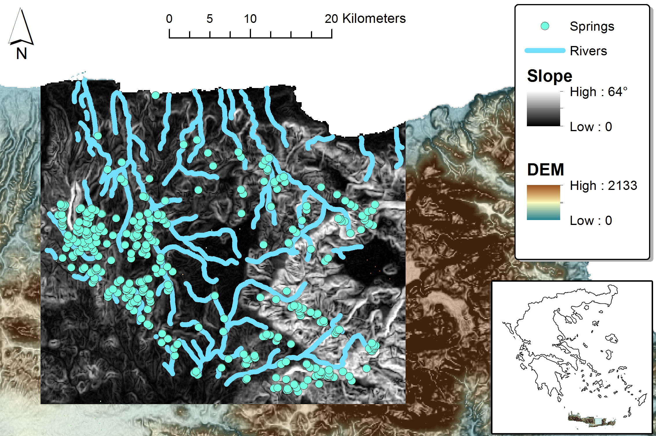
The environment is considered to be the geographic area of the wider region of Knossos, located approximately in central part of the island of Crete. As a result, known habitation sites of the Minoan period where identified, categorized and geolocalized, acquired by the “Digital Crete" project.[9] Agents are located within a 40x30 km area with one (1) hectare cell size for the grid space. Moreover, the environment has also associated data layers representing topographical aspects of the model landscape, such as elevation, slope and aquifer locations, contributing indirectly in agent’s decision-making process, like where to settle and/or cultivate (Figure 4).
Model instantiation
The estimated per hectare population for an agricultural Minoan settlement during the modeled era ranges from 100 up to 400 (Isaakidou 2008). In this work, we assume a density coefficient of 250 people per hectare, that is, the maximum number of inhabitants per grid cell (Driessen 2002). Moreover, the number of household individuals in a given settlement cell is initialized to a random number between 1 and 10. As a consequence, the maximum number of household agents per settlement’s cell is 25, i.e., 250 divided by the maximum number of individuals per household, that is 10. Household and settlements number and location are initialized based on archaeological record, i.e., the number of settlements per scenario is set to 21, which are located at known habitation site locations.
Initial cell resources at a given simulation run are based on archaeological estimates on production yield per hectare (ha) pondered by the agricultural regime employed by the agents. As already noted, agents agricultural regimes, can be either “intensive", producing 1500 kg/ha or “extensive", leading to a production of 1000 kg/ha on an annual basis (Halstead 1981; Jusseret 2010). In this work, we assume that household agents employ an intensive agricultural strategy.
Agent migration radius, that is, the distance that a household agent can migrate to in one time-step is set to the full environmental area (approx. 40 km). An agent may migrate only to a cell where known habitation sites exist, based on the archaeological survey conducted in the specific geographic area. However, we assume a resettlement cost \(rc\) for an agent \(i\), which intuitively reflects the decay of potential resources at destination location with increasing distance:
| $${rc}_i = 1 - e^{- 0.005 \cdot \delta}$$ | (14) |
As a final note, we consider a dynamic population growth, based on the amount of resources consumed by a household agent during the year (Chliaoutakis & Chalkiadakis 2016). This results to a growth rate of about 0.1% when households consume adequate resources, which corresponds to estimated world-wide population growth rates during the Bronze Age (Cowgill 1975; Jones 1999).
Simulation scenarios
We simulate trading across settlements which cultivate the landscape by employing an “intensive farming" agricultural strategy, and deploying the “self-organization" social behaviour, as described in Section 3 . Various scenarios were taken into account for the experimental setup, with different parameterization. Specifically, the main simulation scenarios are for our:
- two spatial interaction models, the XTENT and Gravity ones, and
- two different ways to characterize the importance of settlements, one based on Equation 4, and one based solely on available archaeological data (“site category bias" below)
We note that a natural disaster sub-model (Chliaoutakis et al. 2018) is also incorporated in the ABM, in an attempt to provide insights to whether the effects of the volcanic eruption of Thera (Santorini) affected the trading network behaviour. The natural disaster sub-model takes effect at 1630 BCE, that is, approximately the date of the eruption estimated by earth scientists (Driessen 2019). Tsunami and volcanic ash impact on the artificial society and their effects on agriculture and human life were considered during the conceptualization of the model.
Specifically, a 10 meters sea-level rise (including 2m rise on today’s elevation), with inundations of 300 meters inland are assumed for defining tsunami affected areas on the ABM’s environmental grid, rendering associated agricultural fields useless for up to 20 years. We assume that volcanic ash and pumice has the effect of limiting the production of agricultural fields in the whole model area for up to 10 years. Specifically, ash and pumice are considered to affect environmental cells inversely linear to elevation, since the volcanic ash layer is smaller at higher elevations–i.e. the impact on agricultural output is 100% at zero elevation and 0% at locations with maximum elevation of the area modeled.
Furthermore, the human impact immediately after the Theran volcanic eruption, is assumed to consist of 15% fatalities (a mortality rate due to the event) at the whole environmental area due to one or more earthquakes that the eruption was preceded by, and also due to large amounts of ash and pumice that were emitted. Thus, at the time of the catastrophic event, each individual in our model has a 15% probability of dying.
Simulation results were averaged for each (annual) time-step. Thus, for each scenario, results are averages over 30 simulation runs (repetitions) across a period of 2,000 years (cf. Table 1, Appendix B, for the conventional chronology dates (BCE) of the Minoan period used in our ABM simulation scenarios). Moreover, in all figures below, we depict shaded areas that correspond to 95% confidence intervals around lines corresponding to agent or network characteristics. In order to assist the reader, in all figures the legends are also ranked in accordance to the relative performance of the corresponding agent or trading network behavioural characteristic.
The random number generators introduced in parts of the model are obviously “pseudo-random". Thus, via using the same random “seeds", one may introduce the same opportunities for agents in the model simulations, making thereby our simulations reproducible by any interested party. In terms of simulation time, the process can be quite expensive, since a single run (composed of 2,000 yearly time steps) takes approximately 24 hours on a single core 2.6 GHz computer. However, by employing additional computational power, the simulation process can be sped up significantly; e.g., via allocating a dedicated single-core node of a grid computer to a run, all simulation runs mentioned above can be completed within a few days. Specifically, we utilized the Grid infrastructure of our university, by executing all the above 120 simulation runs on thirty (30) dual-core (2.6GHz) nodes (with 4GB ram each) in just 2 days (as opposed to 4 months on a single-core computer).
We now proceed to discuss our findings regarding the trading network analysis performed on our area and era of interest, based on the spatial interaction models enabled and the available archaeological data.
Simulation results
We begin with presenting our findings regarding the effect of the different spatial interaction models on house- hold agent population, settlements number, and their size. Simulation results are presented in Figure 5 for both the XTENT and Gravity models, considering a low percentage of stored surplus trading scheme, i.e. \(ps\) = 20%, while agents in the model can settle or migrate only to known archaeological site locations at any specific time- step. The 20% \(ps\) value is in our view a realistic assumption for the age and subsistence regimes studied, given that no sea trade is modeled in this work.
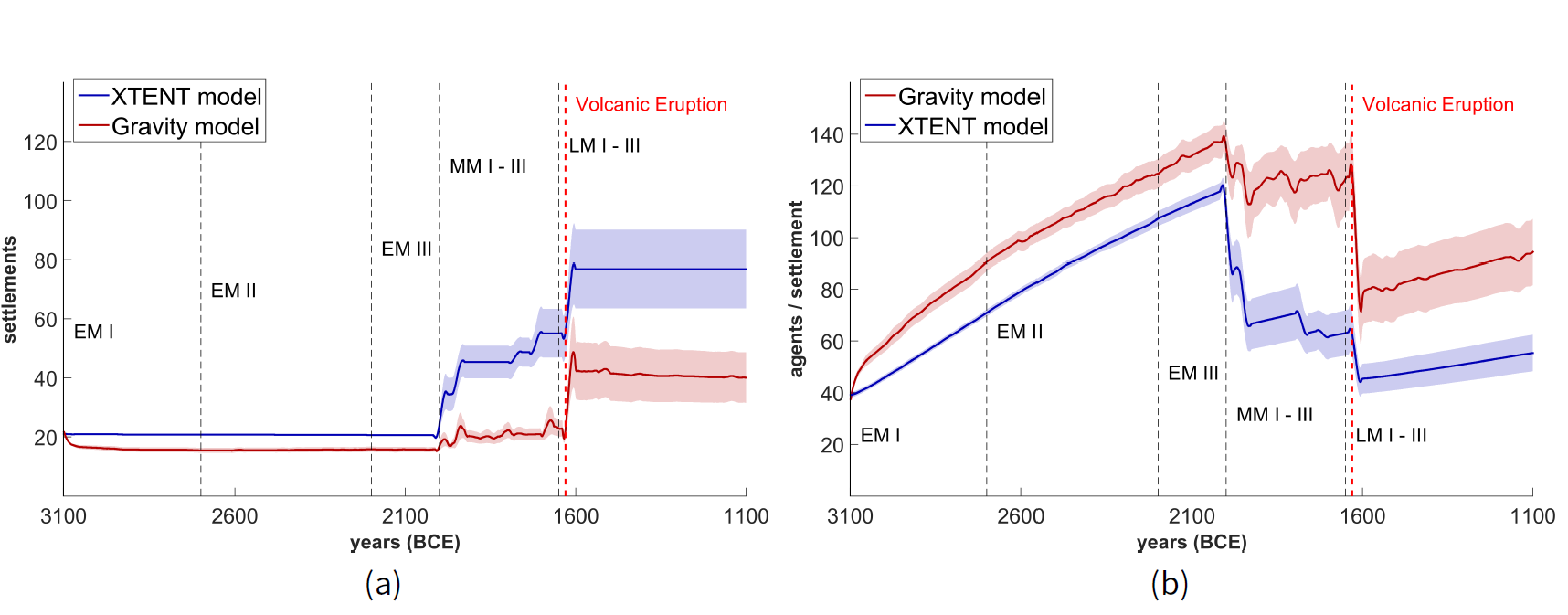
When the XTENT spatial interaction model is used, we observe that the number of settlements remains almost constant until the end of the Early Minoan (EM) period, and then gradually increases over time, especially during the Middle Minoan (MM) period and even more after the volcanic eruption and Late Minoan I (LM I) period (Figure 5a). The number of agents (households) per settlement also appears to increase until the end of the EM period, and then gradually drops in the MM period. Immediately after the volcanic eruption, settlement sizes abruptly drop for a few decades, and start again to gradually increase during LM II and LM III periods (Figure 5b).
Then, when the Gravity model is employed, we observe a similar behaviour with that of XTENT for settlement numbers and sizes, although the number of settlements is slightly lower than the XTENT model during the EM period, and then slowly increases over time, until the end of the MM period (Figure 5a). For both spatial interaction models, however, we observe an increase on settlements number and a gradual decline in settlement sizes during the MM period, due to the availability of a lot more known site locations for migration (cf. Figure 14, Appendix B). We also observe a relatively constant number of settlements after the volcanic eruption until the end of the LM period, with the XTENT model having higher numbers at about 80 settlements and the Gravity model at about 40 settlements on average. On the other hand, the number of agents per settlement is slowly increasing after the volcanic eruption until the end of the LM period, with the Gravity model achieving higher numbers of household agents on average than the XTENT model (Figure 5b).
Overall, a higher number of settlements is observed after the EM period, with an in-parallel decline on the number of households (agents) per settlement. The increasing trend of settlement numbers is in line with the archaeological record, at least until the LM I period, when actual settlement numbers abruptly decline until the beginning of the LM II period (see Figure 14, Appendix B), and then start to increase again until the LM III period.
We also report that the overall household agent population is constantly increasing at a dynamic population growth rate from about 820 initial agents to about 3450 and 2950 agents for the XTENT and Gravity spatial interaction models, respectively, with only an abrupt and short decline immediately after the volcanic eruption Figure 6a. Furthermore, the stored surplus of the agents is gradually decreasing during the whole simulation period, from about one ton to one half of a ton per household for both the XTENT and Gravity spatial interaction models, with only an abrupt increase immediately after the volcanic eruption of Thera; and then again gradually decreases until the end of the LM period Figure 6b. This “shock” on the average storage of households immediately after the volcanic eruption appears to ultimately affect the settlement trading network, since changes in clustering and centralization rates are observed during the LM period, as will be explained later on.
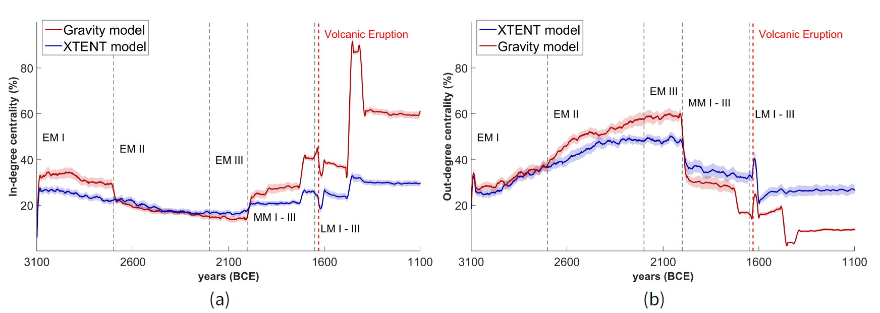
Let us now proceed on the study of the structural behaviour of our settlement trading network. In Figure 7 we present the average relative in-degree and out-degree network graph centralities during the 2,000 years simulation period. When the XTENT model is employed, the relative in-degree graph centrality gradually drops from about 25% to 20% until the end of the EM period (see Figure 7a) while the relative out-degree graph centrality gradually increases from about 20% up to 55% in the same time period (see Figure 7b). Thereafter the relative out-degree graph centrality gradually declines to about 40% until the end of the MM period, abruptly declines[10] immediately after the volcanic eruption to about 20% and then again increases to up to 30% until the end of the LM period. Relative in-degree graph centrality is kept almost constant to about 20% until the end of the LM period, with an abrupt and short decline immediately after the volcanic eruption.

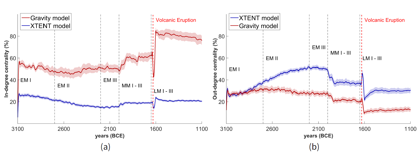
Low relative in-degree graph centrality rates observed during the EM and MM periods (under XTENT) suggest that there are no clearly “prominent" settlements, meaning that, there are no central attractors considering the other settlements in the trading network. On the other hand, the in-parallel high relative out-degree graph centrality rates during the same period, indicate that there are a few settlements that are considered influential in terms of resource distribution. Therefore, one could assume that a settlement organization of distributing resources by these influential settlements in the trading network is implied, at least before the volcanic eruption of Thera or the LM period.
Using the Gravity model, the relative in-degree graph centrality gradually increases from about 40% to 75% until the end of LM period, however, with an abrupt fall and rise immediately after the volcanic eruption (Figure 7a). By contrast, the relative out-degree graph centrality slowly decreases from about 30% to 15% during the whole period, with an abrupt decline immediately after the volcanic eruption (Figure 7b). These high relative in-degree graph centrality rates (under Gravity) suggest that there are only a few “prominent" settlements in the network, implying the possibility of a settlement hierarchy where resources are traded towards these important settlements by other settlements in the trading network. Notice however that this assumes an “attractiveness" of the sites given their Wi importance defined via Equation 4, and not the known category of the archaeological sites. In the next section, we see that the “conclusions" obtained with the Gravity model are quite different when the real sites’ category is taken into account; and that in that case they are more in agreement with those of the XTENT model.
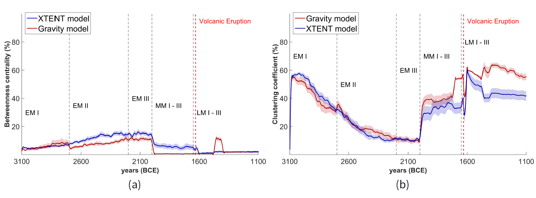
Moreover, the relative graph centrality based on betweenness is considerably low regarding both XTENT and Gravity models, as presented in Figure 8a. This means that most of the trading connections can be made in the trading network without the aid of an intermediary settlement. Thus, there do not appear to exist settlements with much potential of controlling the inter-settlement trade. As such, there is a need to further study if there are other group formation phenomena at work, which need to be captured.
Studying the average clustering coefficient of the trading network graph (Figure 8b), we observe that when the Gravity model is employed, it is relatively low (below 40%) until the beginning of LM period, while it is relatively high after the volcanic eruption (more than 40%) until the end of the LM period. When the XTENT model is employed for the trading process, we observe that the average clustering coefficient of the network graph gradually declines from about 50% to 10% until the end of middle EM period; however, it then gradually increases to about 40% until the end of the LM period, with an abrupt and short fall immediately after the volcanic eruption.
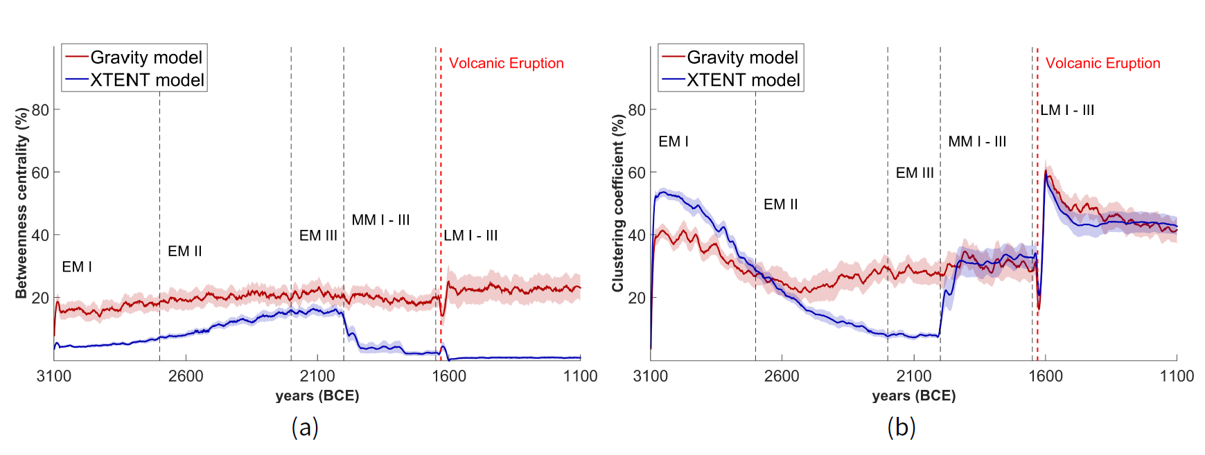
Thus, for both the XTENT and Gravity models, the observed settlement trading clustering behaviour after the volcanic eruption until the end of LM period, implies a more dense trading activity between settlements at the time, raising the possibility of more settlement clusters in the trading network. Assuming that such settlement clusters were around large towns, cities, or palaces, this trading network clustering behaviour has a correspondence to the archaeological record (Figure 14, Appendix B): just two cities are known to have existed during the EM period (Archanes and Knossos), while several large towns, cities and palaces were flourishing in the area during the MM and LM periods (Knossos, Malia, Archanes and Galatas).
Finally, for interest, we also conducted additional experiments considering the same simulation scenarios, however, with a higher percentage of stored surplus trading scheme, i.e. \(ps\) =80%. Simulation results exhibit similar behaviour with no remarkable differences, besides the average storage per household agent, where even lower amounts of resources stored are observed for the scenario of trading a higher portion of stored surplus. Corresponding results figures are presented in Appendix C, since their behaviour is entirely similar with simulation scenarios considering a lower percentage of stored surplus trading scheme. This similarity in the trading behaviour observed in the results where \(ps\) = 80% is justified, since the trading network structure naturally takes into account only the number and density of trading interactions between settlements, and not the volume of resources exchanged within the trading network as well.
In all of the above simulation scenarios, we used attributes relating to settlement’s population and lifetime during the simulation period for calculating the weight of the importance \(W_i\) of a settlement \(i\), given Equation 4. In the following simulation scenarios, we fix the \(W_i\) values with known archaeological site categories. This will enable us compare the settlements trading network and the organization structure developed, based on archaeological estimates on settlement types, with the one autonomously developed during the simulations described above.
Site category bias
Let us first assume a simple, broad classification of settlement types rather than specific site categories, which corresponds roughly to the site hierarchy put forward by Driessen (2002), based on archaeological estimates: village (or settlement or hamlet), corresponding to less than 3.5 ha catchment size, hosting fewer than 88 households / 875 inhabitants on average; city (or large town or town), corresponding to less than 25 ha catchment size, having fewer than 625 households / 6250 inhabitants on average; and palace (or capital town), corresponding to greater than 25 ha catchment size, with more than 625 households / 6250 inhabitants on average. Based on this classification of settlement types, instead of using Equation 4, we express Wi of any settlement point location i as a weight in [0; 1], by mapping the corresponding known archaeological site type[11] as follows:
- \(W_i = 0.5\) when the corresponding archaeological site category is a village,
- \(W_i = 0.7\) when the corresponding archaeological site category is a city, and
- \(W_i = 0.9\) when the corresponding archaeological site category is a palace
As such, the “attractiveness" or the probability of trade for any settlement in the trading network, is biased by the corresponding known archaeological site category. Thus, in the following simulation scenarios, settlement importance is based on archaeological evidence on the settlement type at any given time-step and geographic location. The rest of the experimental setup is exactly the same as the simulation scenarios discussed in the previous section.
To begin with, simulation results on agent settlements number and size are presented in Figure 9 for both the XTENT and Gravity models. We observe that the number of settlements remains relatively constant until the end of the EM period, similarly to the previous scenarios, where settlement importance was calculated by its own dynamic characteristics, i.e., population.
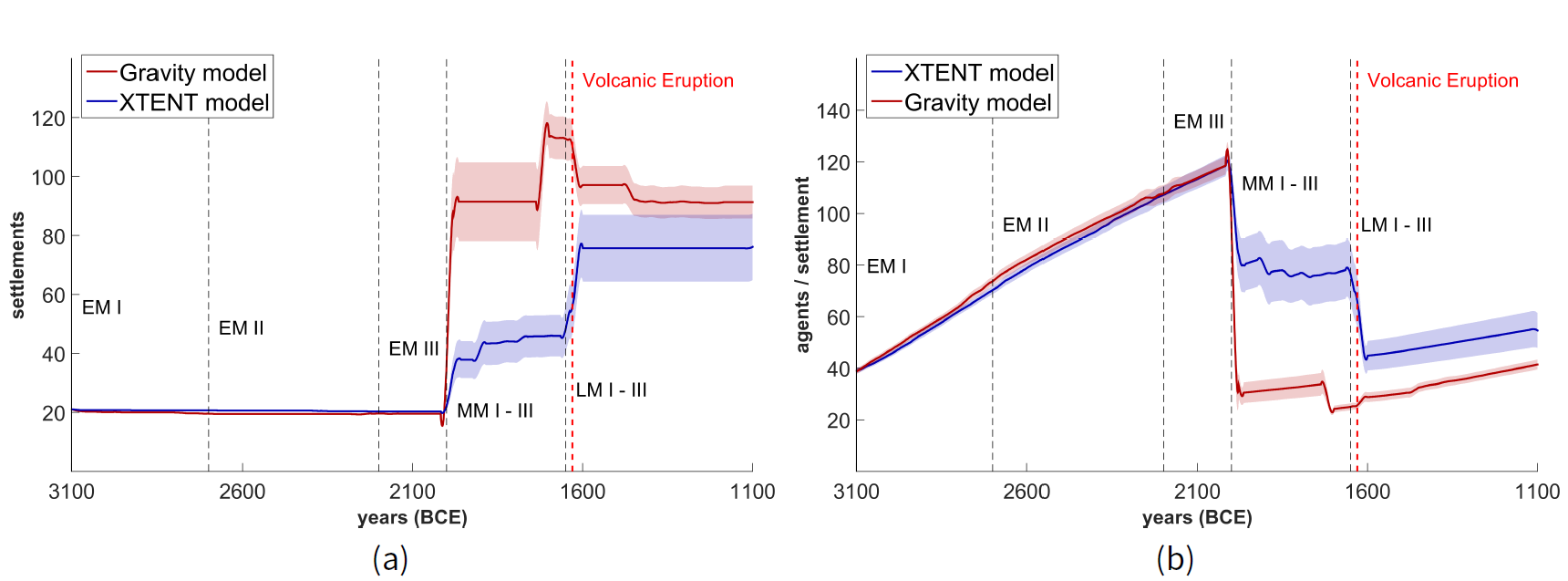
Regarding the XTENT model, we observe a similar behaviour with scenarios not being biased by site categories, where a gradual increase of settlement numbers over time is noticed, especially during the MM period and even more after the volcanic eruption and LM I period (Figure 9a). Similarly, the number of agents per settlement increases until the end of the EM period, and then declines during the MM period. This is due to the high migration rates (because of population growth) observed to more (known) settlement locations available during that period. Moreover, settlement sizes abruptly drop immediately after the volcanic eruption, however, then gradually increase until the end of LM period (Figure 9b).
When the Gravity model is employed, we observe a similar behaviour with the XTENT model in settlement numbers and sizes, although the number of settlements slightly declines at the end of the MM period, and drops further immediately after the volcanic eruption; and then remains relatively constant until the end of the LM period (Figure 9a). Thus, in contrast to the previous scenarios, where no bias by known archaeological site categories was introduced, an entirely different behaviour is now observed. That is, a significant difference in settlement numbers is observed, growing up to about 115 settlements during the end of the MM period, and holding up to about 90 settlements until the end of the LM period, while just a number of about 25 and 40 was observed in the previous scenarios (cf. Figure 5a). We note that this trend in settlement numbers is surprisingly very similar to the one that exists in the archaeological record for the specific environmental area during the whole Minoan period (cf. Figure 14, Appendix B), with the only difference being a substantial decline reported at the end of LM I period in the archaeological record – and which was due to unknown “external" events.[12] Higher values in settlement numbers exist in the archaeological record, suggesting that a higher population growth rate (> 0.1%) probably should have been used during our simulations (we chose to follow Cowgill (1975)).
On the other hand, the numbers of agents per settlement tends to increase until the end of the EM period, and then abruptly declines at the beginning of the MM period from about 120 to 30 households and further decline during the MM III period down to 25. The number of households per settlement, however, is slowly increasing after the volcanic eruption until the end of the LM period, with the Gravity model not being able to achieve higher numbers of household agents per settlement on average than the XTENT model (Figure 9b).
We also report that the overall number of households (i.e., the agent population) is constantly increasing during the whole time period, same as in the scenarios without bias from known archaeological site categories, being able to even achieve higher population sizes, with only an abrupt and short decline immediately after the volcanic eruption (cf. Figure 15 in Appendix C). We note that we observe higher population sizes after the Theran eruption when site category bias is used and the trading network is simulated via the Gravity model (as opposed to XTENT).
Regarding the structural behaviour of the settlement trading network, the relative in-degree and out-degree graph centralities are presented in Figure 10. The XTENT model exhibits a very similar behaviour to the one without known site types bias (cg. Figure 7). Interestingly, the Gravity model is now showing a similar behaviour to the XTENT model, that is, it exhibits lower rates of in-degree and higher rates of relative out-degree centrality. The low relative in-degree graph centrality rates during the EM and MM periods, imply that there are no “prominent" settlements. By contrast, the high relative in-degree graph centrality rates observed in the trading network after the volcanic eruption and during the LM period, suggest that there are certain “prominent" settlements in the trading network. On the other hand, the low relative out-degree graph centrality rates during the LM period, indicate that there are many settlements with a similar degree of “influence" in terms of resource distribution. Therefore, one could assume that a settlement hierarchy where resources are traded towards the (few) most important settlements in the trading network is implied during the LM period.
Moreover, the relative betweenness network centrality is low for both XTENT and Gravity models, as presented in Figure 11a, even lower than scenarios without site category bias (cf. Figure 8a), suggesting even less potential for control on the flow of resources traded between settlements. However, there is a structural basis for assuming that certain settlements with the highest relative betweenness centrality in the society are “different" from the other settlements in the area, at least during the EM and MM period.
Regarding the average clustering coefficient of the trading network graph (Figure 11b), we observe that the Gravity model has again a similar behaviour to the XTENT model, that is, it gradually declines from about 50% to 10% until the end of middle EM period, and gradually increases to more than 50% until the end of the LM period, with an abrupt and short fall immediately after the volcanic eruption. The low clusterization thus observed in the trading network until the end of the EM period may suggest that the trading network connections are losing density until the end of the EM period. The network’s clusterization appears to be recovered in the MM period, and even more in the LM period, indicating the possibility of more dense settlement clusters in the trading net- work, where resources are traded towards the few most important settlements within these clusters (those with high relative in-degree graph centrality). There seems to be a correspondence with the archaeological record, enhancing such a possibility — since several towns, cities or palaces are recorded during the MM and LM period, while just a two towns exist during the EM period, as previously noted.
Concluding this section, we remind here the reader that the Gravity model is able to better capture the trend in settlement numbers that exist in archaeological record. This is a reason to believe that, in this case, Gravity allows us to better interpret the structure and dynamics of the formed trading network. The “unchanged" behaviour of the XTENT model is justified, since it favours the distance between settlements rather than their importance. Thus, it should be used in cases where settlements importance is not known, or cannot be properly modeled.
Conclusions and Future Work
In this work, we presented an archaeology-related ABM to simulate trading interactions across settlements of an artificial past society. The ABM was formally built upon MAS-originating concepts, adopting a utility-based agent design. We model inter-community trading interactions by incorporating a trading sub-model, employing two well-known spatial interaction models, XTENT and Gravity. The simulations’ aim was to assess the sustainability of the artificial society in terms of population size, number and distribution of agent communities with respect to both spatial interaction models; to analyse the resulting trading network structure during its evolution over time; and to draw interesting conclusions (or, rather, sketch out interesting hypotheses) about the settlements’ hierarchy, via annotating our results with the archaeological record.
As a case study we considered the Bronze Age Minoan civilization and as the ABM’s environmental area we considered the geographic area of the wider region around Knossos, located in the central part of the island of Crete, Greece. Simulation results show that when settlements’ importance is known or properly inferred (based on archaeological data or evidence), modeling a trading network relying on the Gravity model can produce settlement patterns similar to the one that exist in archaeological record for the area under study (see Figure 9a). On the other hand, if solely settlement locations are known, then the XTENT model can produce acceptable results on simulating the trading activity between them.
Simulation results show that, when the importance of settlements is weighted based on the type of known archaeological habitation sites, high relative out-degree centrality rates are observed in the trading network, along with low clustering during the end of the EM period. This observation suggests that a small number of influential centres might have existed, linked to a settlement hierarchy where resources are distributed by these centres to other settlements in the network—but with no clearly prominent centres to which resources are directed. Interestingly, after the catastrophic event of the volcanic eruption of Thera and during the LM period, the trading network connections are becoming much denser, and resources are now being distributed towards only a few prominent settlements in the network. We note that these results are in line with archaeological theories suggesting after the MM period the actual settlements hierarchy was transformed, with subsequent radical changes in their trading network, affected by settlement numbers and sizes as well as natural disaster events (as also indicated by Figure 10 and 11 in our work here). Specifically, archaeologists argue that independent political units and centres of the EM and early MM period, were incorporated into a "Knossian" state during late MM and early LM periods by being demoted to secondary centres while others were promoted from tertiary to secondary centres (Driessen 2019). Thus, large and comparatively well integrated polities that existed until the end of the MM period in Central Crete were incorporated into a larger political framework and a territorial state headed by Knossos (Driessen 2002). Given the above simulation results, our ABM appears to be able to provide support for those theories to some extent.
In terms of future work, we need to run more scenarios with a variety of initialization setups. In addition, we intend to equip the ABM with additional modules (vegetation data, geological information, other archaeological evidence or scenarios of interest) and further types of utility-generating activities (fishing, hunting, animal husbandry, crafting), to allow the further integration of qualitative and social factors into our model (Roux 2019). Specifically, we intend to run simulation scenarios where additional resources during the trading process are available from external sources, by building a more elaborate trading model that will also include maritime trade (and its effects in coastal settlements) or trade based on the proximity to religious centres or peak sanctuaries; of course, these components will be also affected differently by the natural disaster sub-model, when it is enabled (i.e. the volcanic eruption of Thera, in this case study). We also intend to represent the dynamic trading network as a “weighted" directed network graph, in order to take into account the amount or volume of resources exchanged during trade, rather than solely the number or density of trading interactions between settlements in the network. Finally, we intend to run simulation scenarios on (artificial) past societies in different geographical space and time, where sufficient archaeological data is available for testing and assessing ABM results with respect to related archaeological hypotheses regarding their social organization.
Acknowledgements
The authors wish to thank the Laboratory of Geophysical - Satellite Remote Sensing & Archaeo - environment (GeoSat ReSeArch) of the Institute for Mediterranean Studies (IMS) / Foundation of Research & Technology (FORTH) for providing archaeological data for the ABM. We particularly thank the archaeologists Dr. Sylviane Déderix, Dr. Gianluca Cantoro and Dr. Stefania Michalopoulou for their valuable comments, suggestions and fruitful discussions.Model Documentation
A detailed model description, following the ODD (Overview, Design concepts, Details) protocol (Grimm et al. 2006) is provided in Appendix D. The ABM was developed using the NetLogo modeling environment (Wilensky 1999). The source code is available at https://www.comses.net/codebases/50cf5d2a-0f37-4d4d-84e0-715e641180d9.Notes
- ABM refers to both agent-based "modeling" and "model(s)".
- A heterarchy is a system of organization where its elements are "unranked" (non-hierarchical) or possess the potential to be ranked by a number of different ways (Crumley 1995).
- We could not conduct further analysis or validation of the specific ABM, since the URL of the ABM source code no longer exists.
- We note that by doing so we do not mean to argue that utility is the main factor driving human behaviour or the advance of human societies. Nevertheless, utility-based agents and utility theory have long been adopted as useful tools in the MAS community (Russell & Norvig 2002; Wooldridge 2009). Therefore, we believe that demonstrating that such notions can be incorporated in archaeology ABMs, as we do in this paper, is interesting from the point of view of the MAS, ABM, and computational archaeology communities alike.
- Households were considered to be the main social unit of production during the period and in the society under study (Whitelaw 2007).
- For details on the definition of \(R\) you may refer to Chliaoutakis & Chalkiadakis (2016).
- More accurately socio-economic social organization paradigms.
- The distance factor \(D_{i,j}\) is measured as the Euclidean (linear) distance for simplicity. This distance can be alternatively measured as the Least Cost Path between two settlement locations, considering slope and elevation as cost surfaces, however, with significantly higher computational cost.
- See http://digitalcrete.ims.forth.gr.
- Short “jumps" observed in the figures immediately after the volcanic eruption are not real, but a result of the Savitzky–Golay smoothing filter applied on the data (Savitzky & Golay 1964). The filter increases the precision of the data without distorting their tendency, by fitting successive sub-sets of adjacent data points with a low-degree polynomial with the method of linear least squares.
- We remind the reader that all potential settlement locations correspond to actual settlement sites.
- Archaeologists assume that a wave of fire destructions affected Cretan settlements during and at the end of LM IB, that have variously been attributed to internal revolt, Mycenaean invasion, or to a major natural disaster involving earthquakes (Driessen 2019).
Appendix
A: Visualizing settlements attraction areas
In the following two figures, each settlement is depicted with a unique coloured circle, where its size represents its importance with respect to its type (village, town or city in this example), while its main trading territory, i.e., landscape cells that are mostly attracted to it, is depicted with the same color.

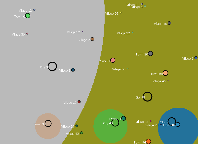
B: Case study’s archaeological record
| Chronology (Platon) | Relative chronology | Manning (1995) | McEnroe (2010) | Simplified date |
| Protominoan Age | EM (Early Minoan) | |||
| Phase I | EM I | 3100 - 2700 | 3100 - | 3100 - 2700 |
| Phsae II | EM II | 2700 - 2200 | - 2200 | 2700 - 2200 |
| Phase III | EM III | 2200 - 2050 | 2200 - | 2200 - 2000 |
| Minoan Age (Palace period) | MM (Middle Minoan) | |||
| Pre-palace | MM IA | 2050 - 1925 | - 1900 | 2000 - 1900 |
| Old-palace Phase I | MM IB | 1925 - 1900 | 1900 - | 1900 - 1875 |
| Old-palace Phase II | MM IIA | 1900 - | - | 1875 - 1800 |
| Old-palace Phase II | MM IIB | -1750 | - 1750 | 1800 - 1720 |
| New-palace Phase I | MM IIIA | 1750 - 1700 | 1750 - | 1720 - 1680 |
| New-palace Phase I | MM IIIB | 1700 - 1675 | - 1700 | 1680 - 1650 |
| LM (Late Minoan) | ||||
| New-palace Phase II | LM IA | 1675 - 1600 | 1700 - 1580 | 1650 - 1550 |
| New-palace Phase II | LM IB | 1600 - 1490 | 1580 - 1490 | 1550 - 1470 |
| New-palace Phase III | LM II | 1490 - 1435 | 1490 - 1360 | 1470 - 1405 |
| Post-palace Phase I | LM IIIA | 1435 - 1360 | 1360 - | 1405 - 1325 |
| Post-palace Phase II | LM IIIB | 1360 - 1200 | - 1200 | 1325 - 1190 |
| Post-palace Phase II | LM IIIC | 1200 - 1100 | 1200 - 1100 | 1190 - 1100 |
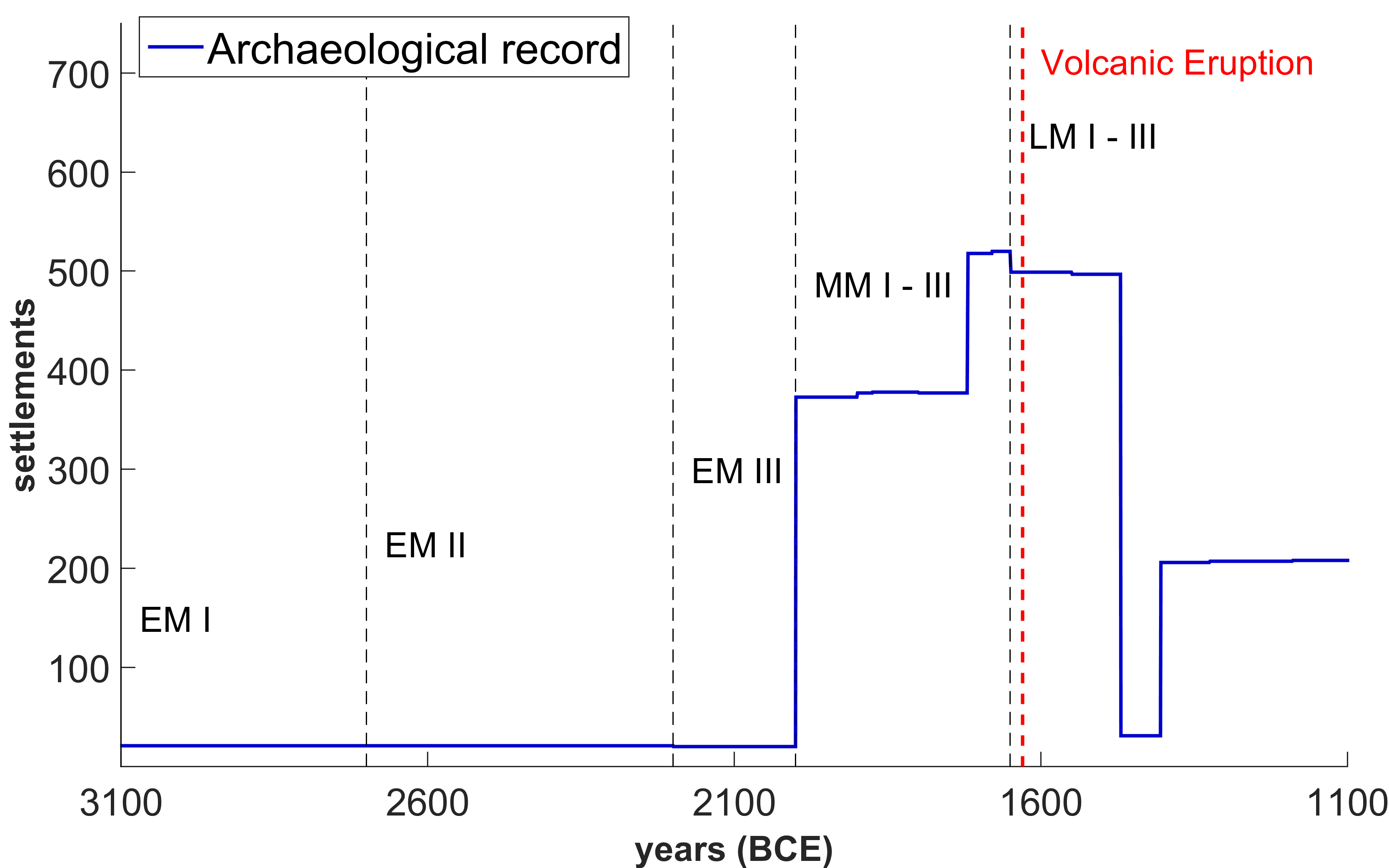
C: Results from additional simulation scenarios
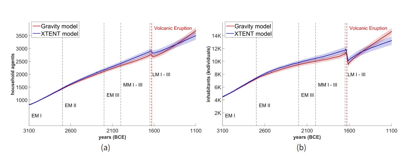
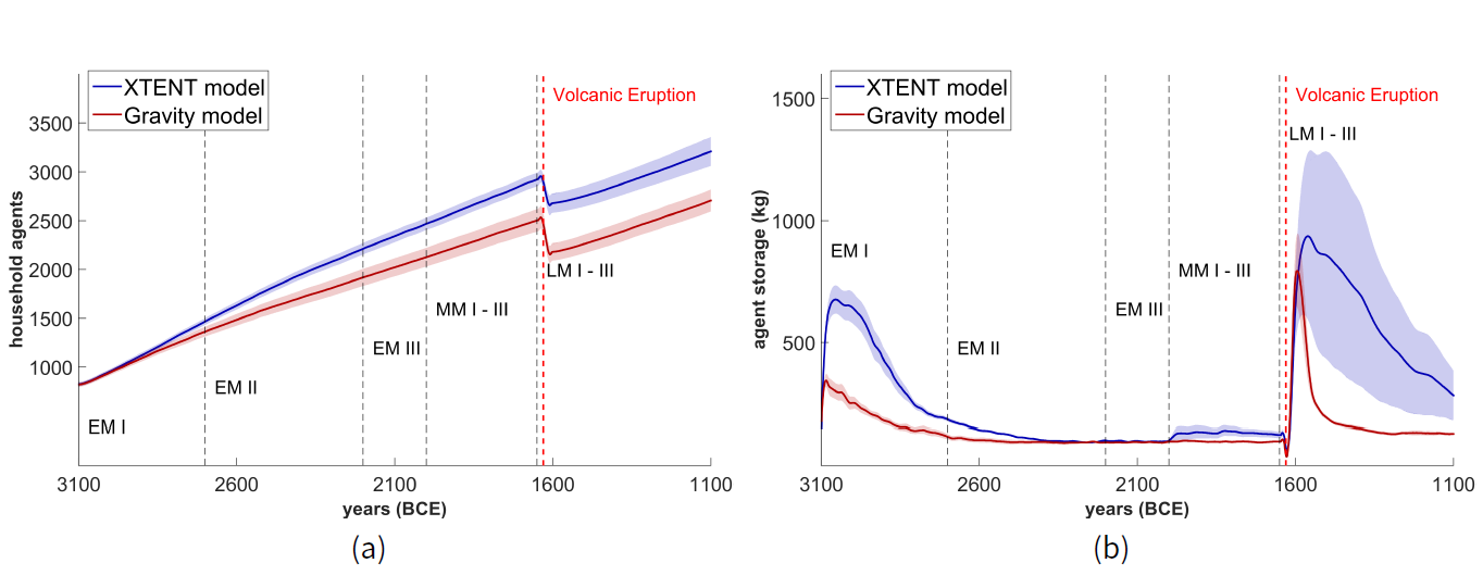
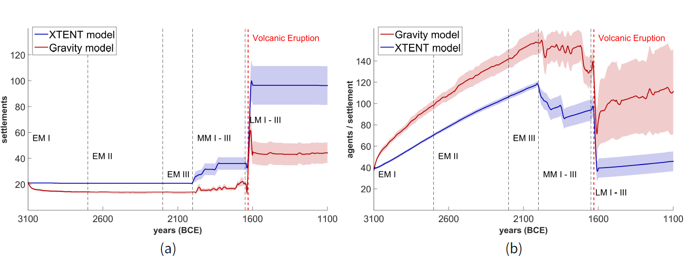
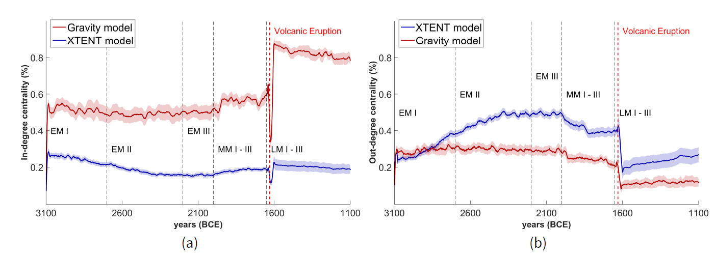

D: ODD protocol for the ABM
The model description follows the ODD (Overview, Design concepts, Details) protocol for describing individual- and agent-based models (Grimm et al. 2006), as updated by Grimm et al. (2010).
Purpose and patterns
Purpose: The purpose of the model is to explore the social organization of an artificial sedentary past society and how different social organization paradigms affect population sustainability and settlements distribution patters. In this work, we study how inter-settlement organization and interactions affect the structural behaviour of the dynamic trading network formulated over time. Specifically, we are addressing the following questions: How a Minoan settlement trading network would look like in the wider area of Knossos, and how does the trading network’s dynamics evolve in response to environmental changes and the anticipated social crisis caused by the volcanic eruption of Thera island? For this purpose, we consider two different approaches for modeling trading interaction probability, corresponding to "attractiveness" among settlements, based on the distance between them and their "importance". As a case study, we consider the "Minoan" civilization and provide in the process insights and potentially support for archaeological hypotheses regarding the settlement organization in the wider area of Knossos in Central Crete, Greece, during the Bronze Age.
Simulation results show that modeling a trading network by favouring settlements importance rather than the distance between them, as with the Gravity model, can produce settlement patterns similar to the one that exist in archaeological record for the area under study. However, such a spatial interaction model should be deployed only when settlements importance is known or properly inferred. In such case, the trading network structure also suggests that a small number of influential centres could have existed until the Early Minoan period. This fact may suggest a settlement hierarchy where resources are distributed by these influential settlements to others in the network, however, with no clearly prominent centres to which resources are directed. In addition, after the volcanic eruption of Thera and during the Late Minoan period, the trading network connections are becoming much denser, with resources being distributed towards only a few settlements in the network.
Patterns: Archaeological estimates for the era and space under study are provided as input in the model, as well as archaeological survey data; in particular, known habitation site locations and types, such as village, city or palace. In our simulation experiments, agents in our environmental grid are allowed to settle or migrate only to cells that actual archaeological habitation sites existed at the specific time (step). Therefore, the patterns observed on settlement numbers during our simulations against the ones observed in the archaeological record, allow us to evaluate the suitability of two different spatial-interaction models, that we used for modeling the interaction probability (attractiveness) among settlements.
Entities, state variables and scales
Entities: The are three main entities that are included in the model: households, settlements and environmen-tal cells. Agents correspond to households, each containing up to a maximum number of individuals (household population). Each household agent resides in a cell within the environmental grid, with the cell potentially shared by a number of agents. Adjacent cells occupied by agents make up a settlement — and there is at least one occupied cell in a settlement. Each agent cultivates a number of cells located next to the settlement. The number of cells that a given household needs (and is able) to cultivate at a given location, depends on the number of its individuals, and its agricultural regime, i.e., "intensive" or "extensive" agriculture.
State variables: The main state variables for a household, besides the current number of its individuals and the settlement that the household belongs to, are: current utility, minimum resources needed, surplus of resources stored, a list of its current cultivating patches, a boolean variable (true/false) for considering migrating to another location, the number of cells that needs to cultivate, the number of years (annual time-steps) that the agent exists within the settlement and in the environment, and others.
The main state variables for a settlement are: a list of the household agents within the settlement; the total number of households and its population (number of people); the weight of its importance; the total amount of resources received by other settlements during trade; the number of years that the settlement exists in the environment; the in-degree, out-degree and betweenness centrality values; and the clustering coefficient regarding the settlement’s position on the trading network.
State variables for environmental cells include static variables, such as elevation and slope data derived from a today’s Digital Elevation Model (DEM) of the modeling area; the land-productivity for the patch (amount of resources) that is based on settlement’s population; the land-suitability that is based on the slope value of the corresponding cell; the utility of an aquifer for the respective cell; the agricultural production (agent reward) of the cell that is based on land suitability and productivity; the initial resources of the cell; and several other parameters denoting if the cell is also an aquifer location, or if a known archaeological habitation site existed in the current time-step (along with site type and derived importance), or if it is currently cultivated, and others.
Scales: Household agents and resources are located within a 40x30 km area, with a 100x100 m (1 ha) cell size for the grid space. Thus, the landscape consists 120K cells. The time slot investigated is 2,000 years (ca. 3100 – 1100 BCE), with annual time-steps.
Process overview and scheduling
Processes: At every time-step, corresponding to a period of one year, household agents first harvest resources located in nearby cells (corresponding to the fields they are cultivating). They then check whether their harvest satisfies their minimum perceived needs. In such a case, potential surplus is added to any stored resource quantities for a specific number of years (user defined parameter). If not, they might ask others for help (depending on the social organization behaviour in effect), or they might even eventually consider moving to another location or settlement, depending on the expected utility for these actions.
Moreover, we assume that each (household) agent within a settlement is socially contracted as a community member to give away a portion of its stored surplus (e.g., 20%) to be communally pooled as the corresponding settlement trading resources and be traded away by the settlement later on. Then, the settlement can trade and exchange resources with any other settlement based on the probability of interaction or "attractiveness" with the other settlement, thus ultimately transforming the trading network structure.
Furthermore, population size affects the land productivity, in two ways: positively, since the continuous occupation or cultivation of an area by a large populace leads to experience and subsequent higher crop yield; and negatively, since it also leads to overexploitation of resources, thus, induce a lower crop yield. Population levels at a given area are affected by migration, as well as natural population change by birth and death of household population. Lower amount of resources reduces birth rate and thus leads to a reduced population size and threatens household agents with extinction.
We also consider a natural disaster that takes effect at a specific year (1630 BCE, estimated by earth scientists) that is, approximately the date of the volcanic eruption of the Thera (the nearby island of Santorini) in an at- tempt to provide insights to whether the natural disaster affected the trading network behaviour and how.
Schedule: The model is developed to cover the needs of the potential organization of an artificial Minoan society, both in the household and settlement level, based on archaeological evidence and data. At every time- step, the following processes take place: first, we get and set known archaeological habitation sites locations and types information on environmental cells from the associated archaeological sites dataset; the respective information need to be available to agents that consider migrating (process) to another location. Then, environmental updates regarding resources and potential cultivation area for the households agents are scheduled. Cultivation (and harvesting) process follows, where the agricultural production, that is agents reward, for each cultivated field is calculated, based on land suitability and productivity. Household agents expected utility is calculated from all their actions (currently cultivation and migration), immediately after considering the social organization paradigm deployed within the settlement. Afterwards, the trading process (resources exchange) across settlements in the model environment is scheduled, based on the spatial interaction model employed (XTENT or Gravity), thus further updating household agents utility along with the trading network structure. Then, updates regarding agents storage, utility, and their associated characteristics are scheduled, followed by updates on population size, affected by a dynamic population growth rate of 0.1%, when households consume adequate resources. Moreover, population size is further updated along with available agricultural re- sources, if the natural disaster sub-model is enabled, by simulating the effects on agriculture and human life of the volcanic eruption of Thera, based on archaeological evidence and estimates. Finally, observer actions, that is plotting graphs and recording necessary variables to output files, take place at the end of every time step.
Design concepts
Our model employs a utility-based agent design that act autonomously towards utility maximization, that can also build and maintain complex social structures. The utility-based agent architecture, introduced by Multi- Agent Systems, can provide a more general performance measure of the agent "well-being", since it allows comparison of the different agent actions-states to exactly how well the agent is in any given time-step (rational utility maximizer). The model also includes several other design concepts:
Emergence: The main outcomes of the model are trading interaction patterns. In particular, how dense the whole settlement trading network is and if it exhibits an accumulative or distributive behaviour in terms of resources towards a few important or influential settlements, respectively. These outcomes emerge from archaeological data introduced in the model, i.e., the spatial distribution of available known archaeological habitation site locations where agents are only allowed to settle or migrate to and, to a lesser extent, from the way settlements importance is defined and modeled, affecting settlements interaction probability.
Adaptation: Household agents exhibit an adaptive behaviour: deciding whether or not to migrate to another location and, if so, selecting a new location based on the agent’s expected utility for the new location; and also a structural adaptation behaviour when the self-organization social paradigm is employed.
The decision of whether to move depends on satisfying the only in-built goal of the household agent, that is, to stay alive; If an agent does not receive the minimum level of resources it requires (utility threshold) for a specified number of years in a row (and the storage is empty), then it considers migrating to another location (or settlement).
When the self-organization social organization paradigm is employed by the households within a settlement, they interact with one another ("gift" exchange) for the proper allocation of resources. This is achieved by adapting the social structure through changes to their relations (re-organization) continuously over time, thus improving their performance as a "group" (vitality of the settlement).
Sensing: Household agents are assumed to know their own attributes, such as their current utility, surplus stored, etc., and its current relation with other households in the same settlement. Agents have also an explicit knowledge of the environment within a radius that is user-defined (model parameter), although we assume a full environmental view for the agents due to the small area modeled (maximum 40 km).
Interaction: There are two main types of interactions in the model, agent-environment and agent-agent interactions. The former describes the interaction of household agents with their environment, while the later describes their interaction with other households (or settlements) in the modeling area.
The interactions related to agent-environment actions that are currently implemented in our model, are cultivation and migration actions. Both actions depend on the agricultural production of an environmental cell that is affected by land suitability, expressed as a decay with increasing slope, and land productivity representing soil fertility and affected by current population size of the settlement (and inspired by the logistic map equation). We note here, that household agents are making a decisions for cultivating a specific number of cells, based on their number of individuals and the agricultural practice in effect, thus allowing them to achieve an acceptable level of resources instead of maximizing it. With this assumption we are able achieve an appropriate trade-off against utility maximization consideration introduced by the agent design. Likewise, a resettlement cost is also introduced during migration decision-making, that is defined as a decay of expected resources at migrate location with increasing distance. Re-settlement cost is intuitively reflecting costs associated with the relocation of the household agent.
The agent-agent interactions are structured in two levels, intra-settlement interactions that are defined based on the social organization paradigm employed by the household agents within a settlement, and inter-settlement interactions, defined by the spatial interaction model deployed.
Stochasticity: Stochasticity is used in two ways. First, the model can be initialized stochastically, regarding the initial number of settlements in the model, initial number of households, number of household individuals, and amount of resources in each cell. These initialization methods are stochastic so that each simulation run for each scenario produces different results. In this work, in particular, only the number of settlements is not stochastically initialized, but rather based on actual number and locations of known archaeological habitation sites at the beginning of our simulation (ca. 3100 BCE). Moreover, there is also an inherent stochasticity introduced by the (NetLogo) modeling environment regarding the way that agents are executing related processes in the model; households agents or settlements are executing each and every process in a random order.
Second, population dynamics are stochastically defined and based on the dynamic population growth rate (model parameter) that is affected by the amount of resources (thus utility) consumed by the household agent during each year. In addition, settlements are trading resources with one another based on their "attractive- ness" (interaction probability) that is affected by the distance between them and their (weight of) importance, and thus the spatial interaction model in effect.
Collectives: This model includes two kinds of collectives: households that are representing groups of inhabitants, and settlements representing groups of households. The collectives are represented as specific entities with their own state variables and behaviours, as defined above at Entities, State Variables, and Scales. These collectives are included in the model because are essential in modeling an artificial human society from the bottom up.
Observation: The model was tested and analysed by recording all entities and model variables, and observe and validate their values process by process. Moreover, at the graphical user interface (GUI) of our model some of these variables are traced at every time-step for quick evaluation, such as the number of households and settlements, population size, average utility and storage (and per settlement), agent migrations and average migrations per (annual) time step, relative graph centrality (in-degree, out-degree, betweenness) and centralization (clustering coefficient), and others. In any case, all non-static variables are recorded and provided in output files for further statistical analysis.
Initialization
The number of households and population size for each household agent are randomly initialized from a sample of a uniform distribution, depending on the maximum number of inhabitants per cell (ha) and individuals per household agent. The amount of resources for each environmental are also randomly initialized from a sample of a normal distribution. In this work, initialization of state variables is intended to be case-specific, that is, an artificial Minoan society at a specific geographical territory of the island of Crete, Greece (the wider area between the archaeological sites of Knossos and Malia). Therefore, the number of settlements is initialized to twenty one (21) placed at specific environmental cells, that correspond to specific geographical locations of known archaeological habitation sites locations, that are provided as input spatial data file (shapefile).
The maximum number of inhabitants per cell (ha) is set to 250 people and the maximum number of individuals per household is set to 10. Regarding the environmental resources, the minimum amount of resources required per individual per year was set to 250 kg, while households employ an intensive agricultural practice leading to a production of maximum 1,500 kg /ha. All these parameters are based on archaeological estimates for the period and area under study (Halstead 1981; Isaakidou 2008; Jusseret 2010). Moreover, environmental cells state variables, such as elevation and (derived) slope (raster DEM), or aquifer locations (shapefile) are also provided as input spatial data files to the model.
Various scenarios are taken into account for the experimental setup, with different parameterization regarding the two spatial interaction models, XTENT and Gravity, and the two different ways to characterize the importance of settlements; based on population and the settlement’s lifetime or solely on available archaeological data provided as input to the model.
Input data
As already noted, an agent may migrate only to a cell where known archaeological habitation sites existed in the specific time step, based on the archaeological survey conducted in the specific geographic area. The specific geographical locations of known archaeological habitation sites locations (and types) are provided as input spatial data file (shapefile) and used by the model during the simulation to map known site locations to available migrate locations for the household agents.
Submodels
Besides the settlements trading submodel, two other submodels are included in our ABM: the social organization of household agents within a settlement, in particular the self-organization social behaviour, and the natural disaster submodel. Detailed descriptions for the last two submodels are provided in previous work and versions of our ABM. Please refer to Section 4 for the trading submodel and to Chliaoutakis & Chalkiadakis (2016) for the self-organization algorithm and Chliaoutakis et al. (2018) for details on the volcanic eruption submodel.
References
AXTELL, R. L., Epstein, J. M., Dean, J. S., Gumerman, G. J., Swedlund, A. C., Harburger, J., Chakravarty, S., Hammond, R., Parker, J. & Parker, M. (2002). Population growth and collapse in a multiagent model of the Kayenta Anasazi in Long House Valley. Proceedings of the National Academy of Sciences of the United States of America, 99, 7275–7279. [doi:10.1073/pnas.092080799]
BARNES, J. et al. (2014). Complete Works of Aristotle, Volume 1: The Revised Oxford Translation, vol. 1. Ed. by J. Barnes. Princeton, NJ: Princeton University Press.
CHERRY, J. (1986). Polities and Palaces: Some Problems in Minoan State Formation. In Peer Polity Interaction and Socio–Political Change (pp. 19–45). Cambridge, MA: Cambridge University Press.
CHLIAOUTAKIS, A. & Chalkiadakis, G. (2016). Agent-based modeling of ancient societies and their organization structure. Autonomous Agents and Multi-Agent Systems, 30(6), 1072–1116. [doi:10.1007/s10458-016-9325-9]
CHLIAOUTAKIS, A. & Chalkiadakis, G. (2017). Evolutionary Game-theoretic Modeling of Past societies’ Social Organization. The 2018 Conference on Artificial Life: A Hybrid of the European Conference on Artificial Life (ECAL) and the International Conference on the Synthesis and Simulation of Living Systems (ALIFE), (pp. 98–105). [doi:10.7551/ecal_a_020]
CHLIAOUTAKIS, A. & Chalkiadakis, G. (2019). ‘AncientS-ABM: A Novel Tool for Simulating Ancient Societies.’ In Y. Demazeau, E. Matson, J. M. Corchado & F. De la Prieta (Eds.), Advances in Practical Applications of Survivable Agents and Multi-Agent Systems: The PAAMS Collection (pp. 237–241). Berlin/Heidelberg: Springer. [doi:10.1007/978-3-030-24209-1_21]
CHLIAOUTAKIS, A., Chalkiadakis, G. & Sarris, A. (2018). Employing Agent-based Modeling to Study the Impact of the Theran Eruption on Minoan Society. In Spreading Excellence in Computer Applications for Archaeology and Cultural Heritage. Proceedings of the 3rd Conference on Computer Applications and Quantitative Methods in Archaeology - Creece (pp. 139–148).
COCKBURN, D., Crabtree, S. A., Kobti, Z., Kohler, T. A. & Bocinsky, R. K. (2013). Simulating Social and Economic Specialization in Small-Scale Agricultural Societies. Journal of Artificial Societies and Social Simulation, 16(4), 4 :https://www.jasss.org/16/4/4.html. [doi:10.18564/jasss.2308]
COWGILL, G. L. (1975). On the causes and consequences of ancient and modern population changes. American Anthropologist, 77(3), 505–525. [doi:10.1525/aa.1975.77.3.02a00030]
CRABTREE, S. A., Bocinsky, R. K., Hooper, P. L., Ryan, S. C. & Kohler, T. A. (2017). How to make a Polity in the Central Mesa Verde Region. American Antiquity, 82(1), 71–95. [doi:10.1017/aaq.2016.18]
CRUMLEY, C. L. (1995). Heterarchy and the Analysis of Complex Societies. Archeological Papers of the American Anthropological Association, 6(1), 1–5. [doi:10.1525/ap3a.1995.6.1.1]
DEAN, J. S., Gumerman, G. J., Epstein, J. M., Axtell, R. L., Swedlund, A. C., Parket, M. T. & McCarroll, S. (2000). Understanding Anasazi cultural change through agent-based modeling. In T. A. Kohler & G. J. Gumerman (Eds.), Dynamics in Human and Primate Societies (pp. 179–206). Oxford: Oxford University Press. [doi:10.1515/9781400842872.90]
DORAN, J., Palmer, M., Gilbert, N. & Mellars, P. (1994). ‘The EOS Project: Modelling Upper Plaeolithic Social Change.’ In In J. Doran & N. Gilbert (Eds.), Simulating Societies: the Computer Simulation of Social Phenomena. London: UCL Press. [doi:10.4324/9781351165129-9]
DRIESSEN, J. (2002). ‘History and hierarchy. Preliminary observations on the settlement pattern of Minoan Crete.’ In K. Branigan (Ed.), Urbanism in the Aegean Bronze Age (pp. 51–71). New York, NY: Academic Press.
DRIESSEN, J. (2019). The Santorini eruption. An archaeological investigation of its distal impacts on Minoan Crete. Quaternary International, 499, 195–204. [doi:10.1016/j.quaint.2018.04.019]
DRIESSEN, J. & Langohr, C. (2014). Recent Developments in the Archaeology of Minoan Crete. Pharos, 20(1), 75–115.
FREEMAN, L. C. (1979). Centrality in Social Networks Conceptual Clarification. Social Networks, 1(3), 215–239 . [doi:10.1016/0378-8733(78)90021-7]
GRAEBER, D. (2011). Debt: The First 5000 Years. New York, NY: Melville House.
GRAHAM, S. (2006). TravellerSim: Growing Settlement Structures and Territories with Agent-Based Modeling. In Digital Discovery. Exploring New Frontiers in Human Heritage. Proceedings of the 34th Conference on Computer Applications and Quantitative Methods in Archaeology, (pp. 45–59). Archaeolingua.
GRIMM, V., Berger, U., Bastiansen, F., Eliassen, S., Ginot, V., Giske, J., Goss-Custard, J., Grand, T., Heinz, S. K., Huse, G., Huth, A., Jepsen, J. U., Jørgensen, C., Mooij, W. M., Müller, B., Pe’er, G., Piou, C., Railsback, S. F., Robbins, A. M., Robbins, M. M., Rossmanith, E., Rüger, N., Strand, E., Souissi, S., Stillman, R. A., Vabø, R., Visser, U. & DeAngelis, D. L. (2006). A standard protocol for describing individual-based and agent-based models. Ecological Modelling, 198(1), 115 – 126. [doi:10.1016/j.ecolmodel.2006.04.023]
GRIMM, V., Railsback, S. F., Vincenot, C. E., Berger, U., Gallagher, C., DeAngelis, D. L., Edmonds, B., Ge, J., Giske, J., Groeneveld, J., Johnston, A. S., Milles, A., Nabe-Nielsen, J., Polhill, J. G., Radchuk, V., Rohwäder, M.-S., Stillman, R. A., Thiele, J. C. & Ayllón, D. (2020). The ODD Protocol for describing agent-based and other simulation models: A second update to improve clarity, replication, and structural realism. Journal of Artificial Societies and Social Simulation, 23(2), 7: https://www.jasss.org/23/2/7.html. [doi:10.18564/jasss.4259]
HALSTEAD, P. (1981). ‘Counting sheep in Neolithic and Bronze Age Greece.’ In G. I. Hodder & N. Hammond (Eds.), Pattern of the Past: Studies in Honour of David Clarke (pp. 307–39). Cambridge, MA: Cambridge University Press.
HAMILAKIS, Y. (1996). Wine, Oil and the dialectics of power in Bronze Age Crete: A review of the evidence. Oxford Journal of Archaeology, 15, 1–32. [doi:10.1111/j.1468-0092.1996.tb00071.x]
HANNEMAN, R. A. & Riddle, M. (2005). Introduction to Social Network Methods. Riverside, CA: University of California.
HECKBERT, S. (2013). MayaSim: An agent-based model of the Ancient Maya social-ecological system. Journal of Artificial Societies and Social Simulation, 16(4), 11: https://www.jasss.org/16/4/11.html. [doi:10.18564/jasss.2305]
HUFF, D. L. (1964). Defining and Estimating a Trading Area. Journal of Marketing, 28(3), 34–38. [doi:10.1177/002224296402800307]
ISAAKIDOU, V. (2008). The fauna and economy of Neolithic Knossos’ revisited. In Escaping the Labyrinth. The Cretan Neolithic in Context. Sheffield Studies in Aegean Archaeology (pp. 90–114). Oxford: Oxbow Books.
JANSSEN, M. A. (2009). Understanding Artificial Anasazi. Journal of Artificial Societies and Social Simulation, 12(4), 13: https://www.jasss.org/12/4/13.html.
JANSSEN, M. A. (2010). Population aggregation in ancient arid environments. Ecology and Society, 15(2), 19.
JONES, D. W. (1999). The conundrum of Greek population growth in the 8th century B.C.: burials, settlements, and wells. In Opuscula Atheniensia XXIV, vol. 24, 25–50. Astrom Editions.
JUSSERET, S. (2010). Socializing geoarchaeology: insights from Bourdieu’s theory of practice applied to Neolithic and Bronze Age Crete. Geoarchaeology, 25, 675–708. [doi:10.1002/gea.20329]
KOHLER, T. A. (2012). Modeling agricultural productivity and farming effort. Emergence and Collapse of Early Villages: Models of Central Mesa Verde Archaeology, 85–112. [doi:10.1525/california/9780520270145.003.0006]
KOTA, R., Gibbins, N. & Jennings, N. R. (2009). Self-Organising Agent Organisations. In Proc. of AAMAS’09, 797–804.
MANNING, S. W. (1995). The absolute chronology of the Aegean Early Bronze Age: Archaeology, radiocarbon, and history. Continuum International Publishing Group – Sheffie.
MCENROE, J. C. (2010). Architecture of Minoan Crete: Constructing Identity in the Aegean Bronze Age. Austin, TX: University of Texas Pres.
RENFREW, C. & Bahn, P. (2012). Archaeology: Theories, Methods, and Practice. London, UK: Thames and Hudson, 6th edn.
RENFREW, C. & Level, E. V. (1979). Exploring Dominance: Predicting Polities from Centers. In C. Renfrew & K. L. Cooke (Eds.), Transformations (pp. 145–167). New York, NY: Academic Press. [doi:10.1016/b978-0-12-586050-5.50016-6]
RODRIGUE, J.-P., Comtois, C. & Slack, B. (2017). The Geography of Transport Systems. London, UK: Routledge.
ROUX, V. (2019). Modeling the Relational Structure of Ancient Societies through the Chaîne opératoire: The Late Chalcolithic Societies of the Southern Levant as a Case Study. In M. Saqalli & M. Van der Linden /Eds.), Integrating Qualitative and Social Science Factors in Archaeological Modelling, (pp. 163–184). Berlin/Heidelberg: Springer. [doi:10.1007/978-3-030-12723-7_7]
RUSSELL, S. J. A. & Norvig, P. A. (2002). Artificial Intelligence: Modern Approach (2nd ed.). Upper Saddle River, NJ: Prentice Hall Series In Artificial Intelligence.
SAVITZKY, A. & Golay, M. J. (1964). Smoothing and Differentiation of Data by Simplified Least Squares Procedures. Analytical chemistry, 36(8), 1627–1639. [doi:10.1021/ac60214a047]
TOMKINS, P. & Schoep, I. (2010). The Early Bronze Age: Crete. In The Oxford Handbook of the Bronze Age Aegean (pp. 66–82). Oxford, UK: Oxford University Press.
WATTS, D. J. & Strogatz, S. H. (1998). Collective dynamics of ‘small-world’networks. Nature, 393(6684), 440. [doi:10.1038/30918]
WELLMAN, M. P. (2016). Putting the Agent in agent-based modeling. Autonomous Agents and Multi-Agent Systems, 30(6), 1175–1189. [doi:10.1007/s10458-016-9336-6]
WHITE, D. R. & Borgatti, S. P. (1994). Betweenness centrality measures for directed graphs. Social Networks, 16(4), 335–346. [doi:10.1016/0378-8733(94)90015-9]
WHITELAW, T. (2007). ‘House, households and community at Early Minoan Fournou Korifi: Methods and models for interpretation.’ In R. Westgate, N. Fisher & J. Whitley (Eds.), Building Communities: House, Settlement and Society in the Aegean and Beyond, 15 (pp. 65–76). London, UK: British School at Athens Studies.
WILENSKY, U. (1999). Netlogo. Tech. rep., Center for Connected Learning and Computer-Based Modeling, Northwestern University, Evanston, IL: http://ccl.northwestern.edu/netlogo.
WOOLDRIDGE, M. (2009). An Introduction to MultiAgent Systems (2nd ed.). Colchester, UK: Wiley.