
Introduction
Essentially, a metamodel (MM) is a model which describes the behaviour of an original model on a higher hierarchical level (Moorcroh et al. 2001; Urban 2005; Gore et al. 2017). In the context of mechanistically detailed and therefore often computationally expensive agent-based models (ABM) or individual-based models (IBM[1]), MMs provide an efficient way to facilitate profound model analysis and prediction of ABM behaviour over a wide range of parameter combinations.
The term MM originates from the Design of Experiments literature (Wang & Shan 2007; Montgomery 2009). It was originally developed to study the effects of a set of explanatory variables on a response variable. Therein, optimization via response surface MMs was the most widely performed application (Barton 1994). Both terms, surrogate models (Dey et al. 2017) or emulators (Conti & O’Hagan 2010), can also be understood as MMs. Most commonly, they all treat a particular ABM as a white, grey or black box (Papadopoulos & Azar 2016) and link the input and output values by aggregated functions (Barton 1994; Friedman & Pressman 1988; Friedman 1996; Barton & Meckesheimer 2006). As a result, MM significantly reduce simulation costs in terms of computational time and allow easier communication and understanding of simulation models’ behavior (Kleijnen & Sargent 2000; Mertens et al. 2017). This review will not consider other related concepts of MMs such as the model framework of concepts (Goldspink 2000).
The aim of this review is to condense available information about common MM types used for various tasks related to ABM analysis and applications to guide modelers in choosing an appropriate MM type for their research problem. For detailed information on specific MMs and their applications, it is advised to look for reviews or tutorials elsewhere like Barraquand & Murrell (2013), Barton (1994), Gore et al. (2017), Heard et al. (2015), Kalteh et al. (2008), Mertens et al. (2017), O’Hagan (2006), Oakley (2002) or Urban (2005). A methodology for rating MM quality and implementation effort in an ABM context was developed and applied for the reviewed publications by eight different raters with varying mathematical skills and scientific backgrounds. This was done to support readers in their selection and application of an MM in an ABM context.
Methods
Searching procedure
We conducted a literature survey in Open Access databases (see Table 1) on the 17th, 18th, 21st and 24th of January 2019 and considered only peer-reviewed papers. For each database used, we performed ten searches combining the terms agent-based model and individual-based model with each of the following keywords: Approximation, emulator, metamodel, meta-model and surrogate. We did not limit the time frame of the results but took only a maximum of 50 results per search into account, sorted by their relevance. Papers containing a single or combinations of keyword(s) in their title, abstract, or keywords section were selected for review.
| Database | Website |
| Academic Search Complete | ebscohost.com/academic/academic |
| search-complete Web of Science Core Collection | apps.webofknowledge.com |
| Google Scholar | scholar.google.de |
| Scopus | elsevier.com/solutions/scopus |
Categorization of MMs and purpose of application
In contrast to Papadopoulos & Azar (2016), we do not sub-classify MMs into white (reduced order), gray (both physical equations and stochastically estimated parameters) and black box (Machine Learning) surrogate models. Instead, we simply distinguish them according to their approach to describe the link between input and output variables as deterministic (e.g. Differential Equation) and stochastic (e.g. Machine Learning) MMs, respectively. We thus assign, for example, a Partial Differential Equation used for upscaling (e.g. Moorcroh et al. 2001) to the family of deterministic MMs, whereas Bayesian Emulators applied for calibration (e.g. Bijak et al. 2013) are considered as stochastic MMs.
The MMs were first subdivided into two main classes namely deterministic and stochastic models depending on whether they consider probability distributions linked to the input, output, or processes described by the ABM. The classes were further subdivided into six model families that comprise different MM types (Table 2). In this sense, all MM family names resemble the so-called suitcase phrases and do not necessarily share all attributes or requirements of their namesake in a mathematical context. The names of the model types were directly extracted from the accepted papers without any adjustments. Appendix A provides complete information about the reviewed papers and the corresponding model families and types.
We categorized the purpose of each MM exclusively based on the declaration of the particular authors (Table 3). Notably, we understand parameter fitting as calibration incorporating calibration, parameterization or optimization in accordance to Railsback & Grimm (2012).
Assessment of MM quality and implementation effort
In the following paragraphs, we briefly describe how we rated the MM’s quality and implementation effort. For more in-depth information on the procedure as well as for some examples of each rating criterion, see Appendix C. This guide was used to rate each MM application and to calculate the mean quality and implementation effort. An inter-rater reliability was calculated using the icc function of the R package irr version 0.84.1 (Gamer et al. 2019). Following Koo & Li (2016), we applied a two-way mixed effects model (all selected raters were the only one of interest), using average as type (we want to use the mean ratings for each MM application) and agreement as definition since we had sought to evaluate the agreement among the raters.
| Model Class | Model Family | Model Type |
| Deterministic | Ordinary Functional Equation Differential Equation | Difference Equation, Equation-free Modeling, System Dynamics Model Compartment Ordinary Differential Equation (CODE), Ordinary Differential Equation (ODE), Partial Differential Equation (PDE) |
| Stochastic | Regression | First-order Regression, Linear Regression, Polynomial Regression, Weighted Ordinary Least Squares Regression |
| Bayesian Emulator | Approximate Bayesian Computation (ABC), Dynamic Linear Model Gaussian process, Gaussian Process, Spatial Correlation (Kriging), Parametric Likelihood Approximation | |
| Machine Learning | Decision Tree, Decision Tree Ensemble, Feature Selection, Radial Basis Function Network, Random Forest, Support Vector Regression, Symbolic Regression | |
| Markov chain | Transition Matrices |
| Purpose | Description |
| Calibration | Find reasonable values for input parameters (Friedman & Pressman 1988; Barton 1994; Friedman 1996; Kleijnen & Sargent 2000; Barton & Meckesheimer 2006). |
| Prediction | Predict model behavior for new scenarios or parameter values while replacing the simulation model (Kleijnen & Sargent 2000). Also known as exploratory analysis (Bigelow & Davis 2002), what-if analysis (Barton & Meckesheimer 2006) or exploration / inverse exploration (Friedman & Pressman 1988; Friedman 1996). |
| Sensitivity analysis | Explore model output sensitivity to changes in parameter values (Railsback & Grimm 2012; Thiele et al. 2014; Ligmann-Zielinska et al. 2020). |
| Upscaling | Scale the model to a coarser spatial resolution (Cipriotti et al. 2016) or from individuals to populations (Campillo & Champagnat 2012). |
| Criteria | MM Quality | Key Questions | ||
| Low | Medium | High | ||
| Consideration of Uncertainty (CU) | no | yes | with evaluation | Did the authors give any assessment on the uncertainties of the MM assumptions or results? |
| Suitability Assessment (SuA) | none or bad | good (qualitatively) | good (quantitative) | How did the authors state the suitability of the MM for the given purpose? |
| Number of Evaluation Criteria (NE) | 1 | 2 | > 2 | How many different criteria were provided by the authors for evaluating the MM suitability? |
The quality of MM was assessed based on the assessment of the respective source authors using three different criteria (Table 4): Consideration of Uncertainty (CU), Suitability Assessment by Source Authors (SuA), and Number of Evaluation Criteria (NE). With the CU criterion, we evaluated how the authors considered uncertainties in the inputs and outputs of the respective MM family. In this criterion, the term no means that there was no explicit consideration of uncertainty given by the authors using the MM, while yes refers to those where they used at least some (quantitative) measures (e.g. error bars or R2). We assigned a high quality if the source authors had presented measures of uncertainty with a corresponding evaluation of such measures. The term suitability in SuA refers to the applicability of the given MM type (e.g., Approximate Bayesian Computation) to fulfill the particular purpose (e.g., calibration of an ABM). A good MM evaluation by the authors was regarded as medium if the assessment is only based a qualitative statement (e.g., “The MM performed extremely well.”). We adjudged suitability as good in those cases where the ABM emulation was quantitatively assessed with a positive result. The third criteria NE is self-explaining. For example, a basic linear regression model provides two criteria for evaluating suitability (R squared for the goodness of fit and p-value for evaluating the significance of the linear relationship between the input and output variables) and, thus, would receive a medium assessment for this specific criterion if the authors presented those criteria within their peer-reviewed research paper. Example statements like, the MM had a 61% probability of selecting a parameter set that fitted all investigated outputs, or this procedure was successful in 92% of cases, revealing its great potential to assess parameters difficult to measure in nature, were considered as SuA = good with NE = low.
The implementation effort of each MM family was assessed by the following three criteria (Table 5): Availability of Open Access Guiding Sources (AG), R Coverage (RC), and Out-of-the-Box Applicability (OA). Since we focus exclusively on the effort to implement MMs, computational cost has been absent in our consideration. The AG criterion evaluates the effort of finding help or further information for the potential MM application to own needs. If no sources could be found by performing a search in Google Scholar and Google.com using the MM type name as search query, the MM was regarded with a high implementation effort, while multiple usable sources (e.g. a page on Wikipedia.org and a mathematical blog entry) were considered as a medium implementation effort. Low efforts were assessed if there was one source giving a comprehensive tutorial on implementing the respective MM. The RC criterion focused on the free available statistical language R (R Core Team 2018). If one dedicated package is available to implement the whole MM, it was rated with a low implementation effort. If multiple R packages were necessary, a medium effort was given. We assigned a high implementation effort if the entire MM had to be developed from scratch. The last criterion OA assessed the possibility of MMs to be immediately usable (partly depends on the existing software). MMs were evaluated at a high implementation effort if the derivation of specific equations was required or some important assumptions had to be investigated for its use. Little adjustments correspond, for example, to the derivation of a linear model equation for the corresponding R function, while the application of an unsupervised artificial neural network was considered as a low implementation effort.
Using the average value of all raters of each criterion, we conducted an overall assessment of quality and implementation effort of each MM application. Mean ratings were then analyzed separately for quality and implementation effort using the five-level classification (low, low-medium, medium, medium-high and high) displayed in Table 6. If, for example, a MM application received a high SuA, a high NE and a medium CU, a high overall MM quality was given. These overall assessments were used to generate a plot for each application aim (Table 3) depicting the MM quality in the dependency of the MM implementation effort. Within these plots a bisecting line was drawn for visualizing the 1 : 1 ration of quality and implementation effort and highlight favorable MMs scoring above this line and less favorable MMs staying below this line.
| Criteria | Implementation Effort | Key Questions | ||
| Low | Medium | High | ||
| Availability of Open Access Guiding Sources (AG) | 1 good | multiple sources | none | Are there any openly accessible sources like books or blogs that give an implementation guideline for the MM family of interest? |
| R Coverage (RC) | 1 good package | multiple packages | none | Are there any dedicated R packages to implement the given MM? |
| Out-of-the-Box Applicability (OA) | no adjustments | little adjustments | need for full recreation | Is it necessary to develop an own equation from scratch for the MM to be applicable? |
| Amount of Scores in | Overall MM Quality / Implementation Effort | ||
| High | Medium | Low | Level |
| 3 | 0 | 0 | high |
| 2 | 1 | 0 | high |
| 2 | 0 | 1 | medium-high |
| 1 | 2 | 0 | medium-high |
| 1 | 1 | 1 | medium |
| 0 | 3 | 0 | medium |
| 1 | 0 | 2 | low-medium |
| 0 | 2 | 1 | low-medium |
| 0 | 1 | 2 | low |
| 0 | 0 | 3 | low |
Results and discussion
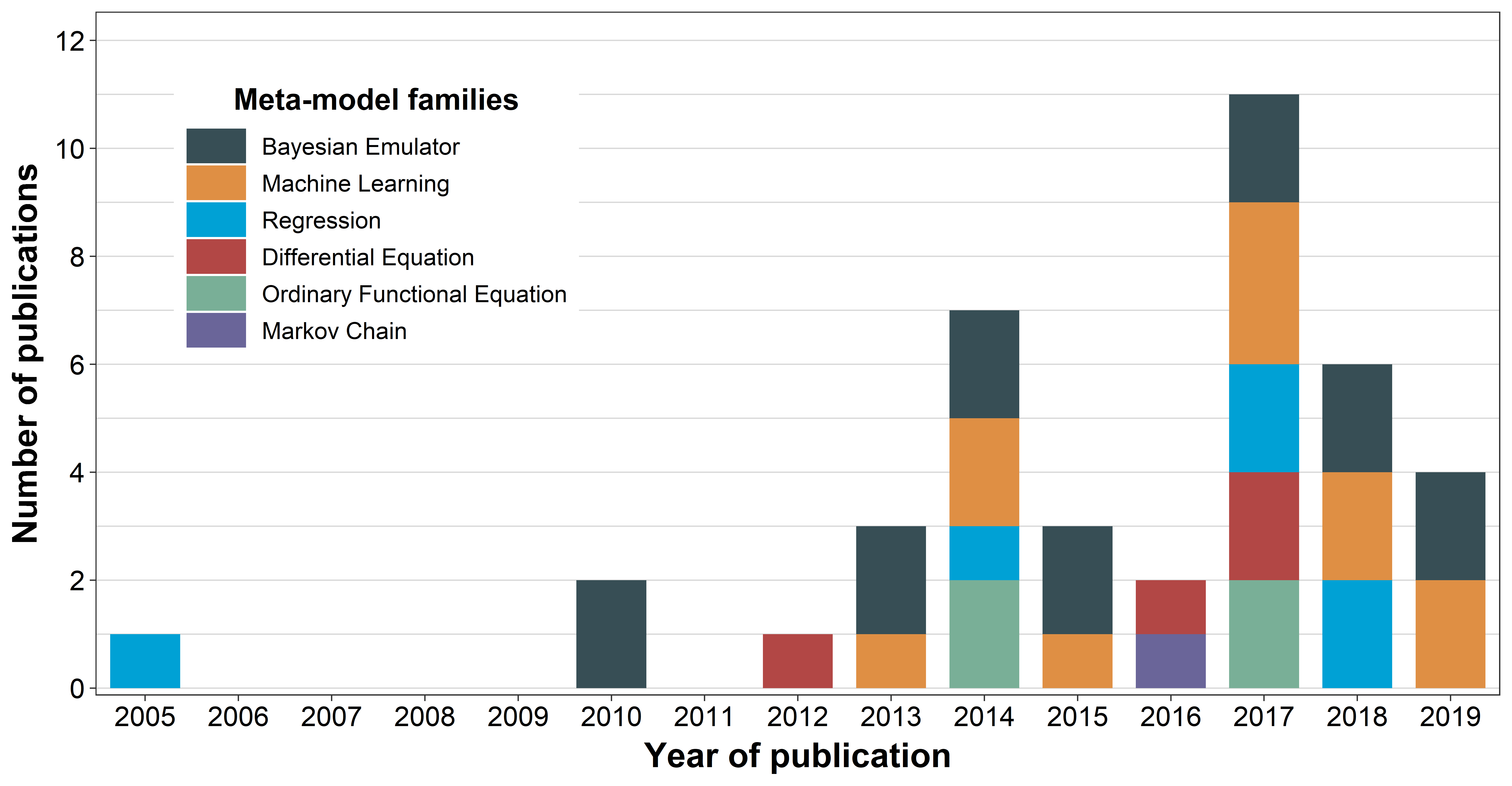
Following the previously described selection criteria (see method section), 27 different peer-reviewed journal papers published from 2005 to 2019 (Figure 1) were accepted for the review (see Appendix B). With this we could extract 40 different MM applications in an ABM context (see Appendix A).
Sensitivity analysis
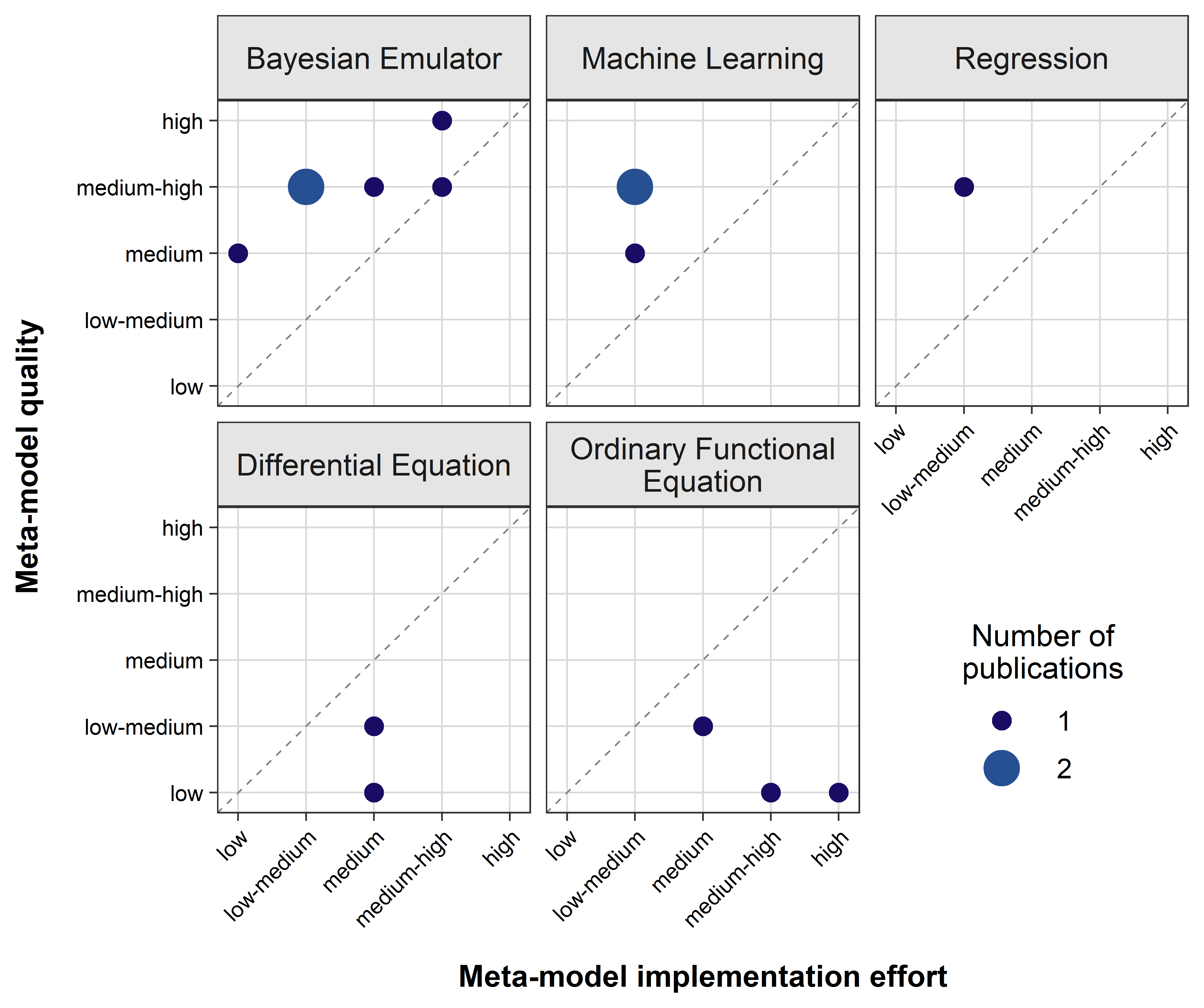
For sensitivity analyses, Bayesian Emulators and Regressions have the highest MM quality indicating accessible implementation efforts (Figure 2). Half of the reviewed publications with focus on Machine Learning scored above the bisecting line indicating a broad MM usage, while the remaining applications were either on or below the bisecting line.
Overall, we found the implementation effort for the three MM families (Bayesian Emulators, Machine Learning and Regression) to be reasonable due to a predominantly high RC (R coverage) and the broad AG (availability of Open Access guiding sources) on these MMs. However, a shortcoming in the application of these three MM families for sensitivity analysis is their need for adjustments to be applicable for another ABM: There was not a single MM type within those MM families that could be reused without any changes. The superior qualities of Bayesian Emulators and Regression MMs result from the moderate to good SuA (Suitability Assessment by Source Authors) in addition to their moderate to good CU (Consideration of Uncertainty). The applied Machine Learning MMs for sensitivity analysis never exceeded a moderate NE (Number of Evaluation Criteria) while their CU and the SuA increased in the following order: Decision Tree Ensemble, Support Vector Regression, Symbolic Regression and Random Forest.

Calibration
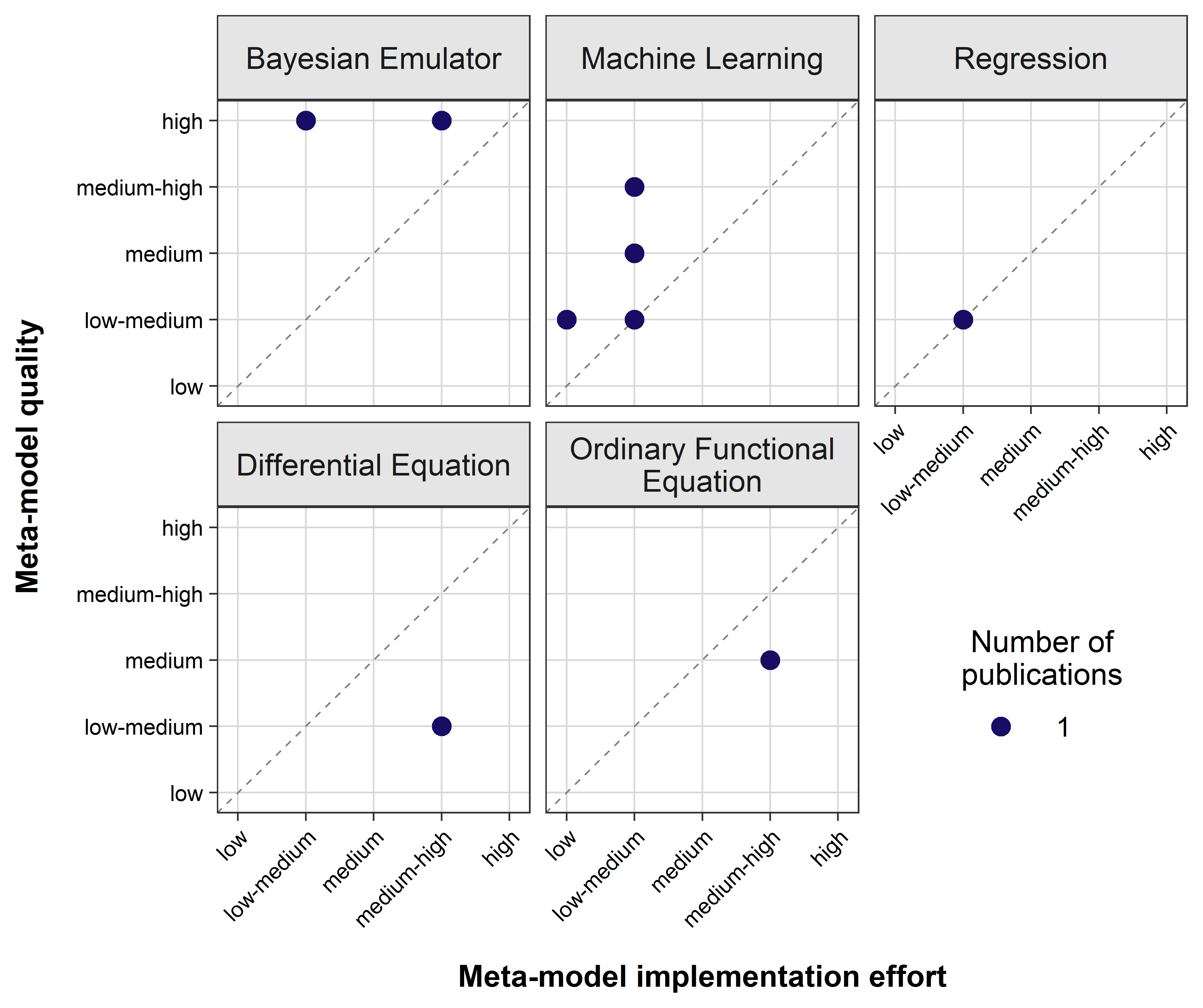
For calibration, Bayesian Emulators, Machine Learning and Regression MMs seem to be the preferable MM families since they constantly stay above the bisecting line (or thereon) indicating a beneficial MM quality to implementation effort ratio (Figure 3). In contrast, Differential Equation and Ordinary Functional Equation MMs do not exceed or even reach the bisecting line and therefore seem to be less favorable MM families to be applied for the purpose of calibrating ABMs.
The overall low-medium implementation efforts of the three best scored MM families such as Bayesian Emulator, Machine Learning and Regression can be explained with their good to at least medium RC (R Coverage) as well as the good to moderate AG (Availability of Guiding Sources). Their OA (Out-of-the-Box Applicability) was never rated as low and always received medium or high assessments regarding their implementation efforts.
High implementation efforts of Differential Equations and Ordinary Functional Equations are due to considerably low OA because they have to be rebuilt entirely for every new ABM. Their AG and RC remain good to medium, emphasizing their broad usability.
The superior MM qualities of Bayesian Emulators are due to their high NE as well as in-depth CU (Consideration of Uncertainty). Only SuA (Suitability Assessment of Source Authors) was poor to medium, indicating that not every MM type of this family suited the task of calibration as good as the others. Machine Learning MMs always achieved a good SuA while their CU and NE (Number of Evaluation Criteria) varied from medium to high.
The considerably poor qualities achieved by Differential Equations and Ordinary Functional Equations result from their low CU and NE. Nevertheless, the respective source authors assessed the suitability of these MMs qualitatively as good.
Prediction
In order to predict the behavior of ABMs, Bayesian Emulators and Machine Learning MMs seem to be the most favorable MM families since they continually exceed the bisecting line of 1 : 1 ratio for MM quality and implementation effort (Figure 4). While the only Regression application for predicting ABMs achieves a low-medium MM quality as well as implementation effort signaling a trade-off between prediction and implementation, Differential Equations as well as Ordinary Functional Equations consistently remain below the bisecting line.
For predicting ABMs behavior, Bayesian Emulators scored the best quality rating with varying implementation efforts. The low-medium effort of Gaussian Process Emulator originates from very good RC (R Coverage) as well as medium OA (Out-of-the-Box Applicability) and AG (Availability of Guiding Sources). The medium-high effort of the dynamic linear model Gaussian Process is due to worse OA, AG as well as RC. The latter two criteria should be considered critically as we used the exact name presented here as a key phrase in our online research while looking for R packages and guiding sources. We could expect a lower implementation effort had we used a more flexible search term for this kind of MM type.
The second best MM family for prediction of ABMs are Machine Learning models. Their considerably low implementation efforts are due to their broad RC and AG. OA varies around a medium ranking with decision trees achieving the highest rating. The varying quality within this MM family is because differentiating SuA (Suitability Assessment) by the respective source authors, while CU (Consideration of Uncertainty) is overall low and NE (Number of Evaluation Criteria) scores between low and medium. The highest quality is achieved by Random Forest for its comparable higher CU and NE.
The Regression MM applied for predicting ABMs is a First Order Regression receiving lower quality ratings while still being good at SuA. The implementation effort consists of a medium OA (the formula of the linear model has to be adapted for every ABM) and a moderate RC, which could be caused by using the whole and exact model name for our online research of R packages.
The overall high implementation efforts of Differential Equations (Compartment Ordinary Differential Equation) and Ordinary Functional Equations (Systems Dynamic Model) while scoring only low-medium to medium qualities are due to their really low OA, since these MM families have to be rebuild anew entirely for each ABM applied. Furthermore, their CU as well as their NE is low, which together with only a qualitatively good SuA add up to medium qualities at best.
Upscaling
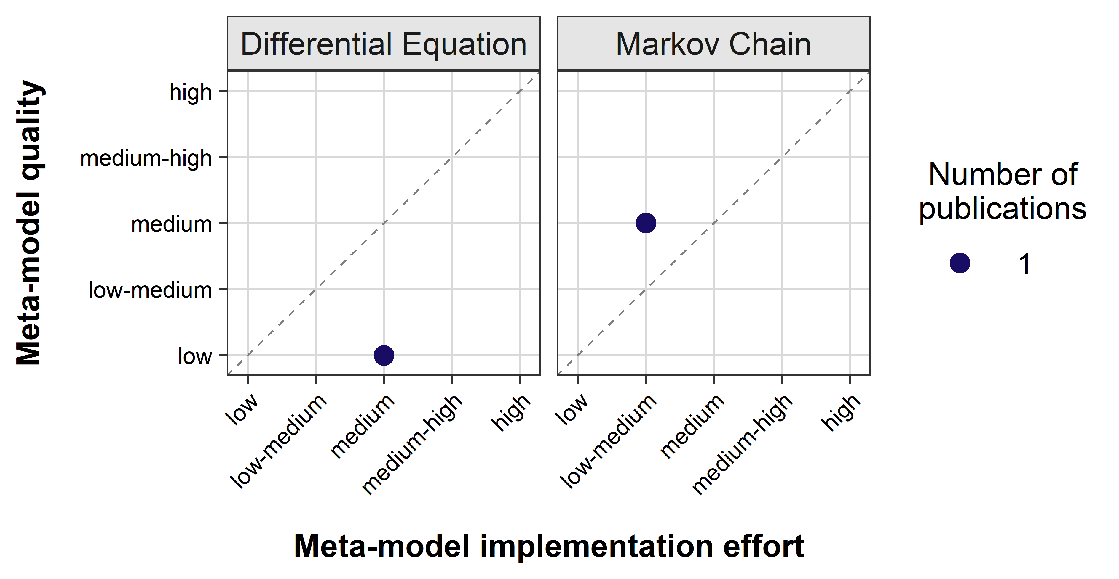
For upscaling ABMs only the Markov Chain MM exceeded a neutral MM quality and implementation effort ratio (Figure 5). The Differential Equation MM stayed below the bisecting line, making it a less favorable choice of MM for upscaling ABMs.
The Markov Chain MM reached a medium quality because of the considerably high SuA (Suitability Assessment by Source Authors), low-medium CU (Consideration of Uncertainty) and NE (Number of Evaluation Criteria). The implementation effort is dominated by its poor OA (Out-of-the-Box Applicability), meaning many adjustments are required to adapt this kind of MM to another ABM. The only accepted Differential Equation (Partial Differential Equation) scored a low OA since a new equation has to be derived for every application in ABMs.
MM rating method and inter-rater reliability
The inter-rater reliability never fell below a fair level and even achieved excellent evaluation for CU (Consideration of Uncertainty) and OA (Out-of-the-Box Applicability) (Table 7).
With eight raters and a sample size of 40 MM applications, the requirements suggested by Koo & Li (2016) are met and exceeded, emphasizing the robustness of the inter-rater reliability results and therewith the results of the MM rating. Nevertheless, the calculated fair intra-class correlation coefficients for SuA (Suitability Assessment of Source Authors), AG (Availability of Guiding Literature) and RC (R Coverage) (Table 7) indicate a necessity to further improve the clarity of the rating instruction for these criteria.
One reason for the stronger variation inside the MM implementation effort criteria AG and RC lies within the diverse backgrounds of the raters which participated in the MM assessment. Since the individual knowledge, the experiences with the corresponding MM types as well as the statistical software R were different (Appendix D), the assessment of a number of R packages needed to apply a given MM varied among reviewers.
The only fair agreement within the MM quality criterion SuA could be because of the unclear instruction for cases in which the authors provided empirical proof for the suitability but never directly assessed it themselves qualitatively. In these cases, some raters gave a medium rating and others a high. Additional divergences emerged when the source authors did not provide any assessment but some raters were able to identify a good or bad fit by themselves while investigating the provided plots, highlighting disparities in certain instances. A more fine grained analysis (e.g. five or seven scale evaluation) might reveal a clustering around high, medium and low with some within variations.
| Rating Category | Rating Criterion | Inter-Rater Reliability | Evaluation |
| MM quality | Consideration of Uncertainty (CU) | 0.859 | excellent |
| Suitability Assessment (SuA) | 0.556 | fair | |
| Number of Evaluation Criteria (NE) | 0.721 | good | |
| MM implementation effort | Availability of Open Access Guiding Sources (AG) | 0.461 | fair |
| R Coverage (RC) | 0.509 | fair | |
| Out-of-the-Box Applicability (OA) | 0.773 | excellent |
Conclusions
Metamodelling is a promising approach to facilitate ABM calibration, sensitivity analysis, prediction and upscaling. We conducted a review that overviews the MM types used among their purposes. Within the 27 papers analysed, we identified 40 different MM applications. For each of them, we (PhD students and Postdocs with none up to moderate mathematical background) assessed the performance quality and the implementation effort. The methodology applied MM rating in this paper was validated by the fair to excellent intra-class correlation coefficients during the inter-rater reliability assessment.
Our goal was to support MM selection for the various needs of daily ABM problems by highlighting the currently most promising MM types with an example each serving as a practical application guide:
- Sensitivity analysis: The easiest MMs to implement with a medium performance are Regression models (e.g. Polynomial Regression Model). Several examples with step-wise guidance for implementation in R (R Core Team 2018) are provided by Thiele et al. (2014).
- Calibration: Approximate Bayesian Computation from the Bayesian Emulator family provides a good balance of effort and performance. Thiele et al. (2014) provides several basic implementation examples of ABM calibration with step-by-step guidance in R (R Core Team 2018).
- Prediction: Gaussian Processes from the Bayesian Emulator MM family provide the best quality while offering low-medium implementation effort. In contrast, Random Forest MMs (Machine Learning family) offer low-medium effort but only medium-high quality. An example on predicting new parameter combinations like an inverted calibration can be found in Peters et al. (2015).
- Upscaling: Transition Matrices from the Markov Chain MM family seem to be the most promising tool for scaling up ABMs. Note that we reviewed only two MMs on this application aim. The corresponding application can be found in Cipriotti et al. (2016).
This review was intended as a ”first aid” for agent-based modelers who seek to improve the performance, optimization or analysis of their simulation model using a metamodel. Our motivation for this work ensued from our day-to-day modeling tasks. Please note that the review presented here can only provide an initial overview, which is primarily meant to stimulate and guide a potential reader through a self-exploration of the wide field of metamodels with ease. The examples presented here are not exhaustive and the field of metamodeling itself is constantly and rapidly developing. Particularly, the application of the potentials offered by various methods of artificial intelligence (with the branches of machine learning or deep learning) is just beginning to emerge. We would therefore like to motivate our readers to stay abreast on new developments in applying metamodeling approach to ABMs, and above all, try out metamodels in their own ways.
Acknowledgements
BP acknowledges funding from the PhD scholarship from the German Federal Environmental Foundation (Deutsche Bundesstihung Umwelt - DBU). SF was supported by the German Research Foundation (DFG project TI 824/3-1).Notes
- We refer to both individual- and agent-based models synonymously as ABM.
Appendix
A: MM classification and evaluation
For the results of MM classification and assessment of implementation effort as well as information quality, see the CSV file labelled "results-rating.csv".
B: Peer-reviewed papers accepted for this review
The complete list of references accepted for this review can be retrieved from the PDF file labelled "reviewed-paper.pdf".
C: MM rating instructions
The methods used for the MM quality and implementation effort rating can be found in the PDF file labelled "rating-instructions.pdf".
D: Rater background information
Information on the background of each rater highlighting their field of expertise, their experiences with R, modeling in general as well as with MMs in detail can be found in the CSV file labelled "background.csv".
References
BARRAQUAND, F. & Murrell, D. J. (2013). Scaling up predator-prey dynamics using spatial moment equations. Methods in Ecology and Evolution, 4(3), 276–289. [doi:10.1111/2041-210x.12014]
BARTON, R. (1994). Metamodeling: A state of the art review. In Proceedings of Winter Simulation Conference, 1987, (pp. 237–244). IEEE.
BARTON, R. R. & Meckesheimer, M. (2006). ‘Metamodel-Based Simulation Optimization.’ In S. G. Henderson, B. L. Nelson (Eds.), Handbooks in Operations Research and Management Science, vol. 13, Amsterdam: Elsevier, pp. 535–574. [doi:10.1016/s0927-0507(06)13018-2]
BIGELOW, J. H. & Davis, P. K. (2002). ‘Developing improved metamodels by combining phenomenological reasoning with statistical methods.’ In A. F. Sisti & D. A. Trevisani (Eds.), Enabling Technologies for Simulation Science VI, vol. 4716. SPIE Digital Library, pp. 167–180. [doi:10.1117/12.474911]
BIJAK, J., Hilton, J., Silverman, E. & Cao, V. D. (2013). Reforging the wedding ring: Exploring a semi-artificial model of population for the United Kingdom with gaussian process emulators. Demographic Research, 29, 729–766. [doi:10.4054/demres.2013.29.27]
CAMPILLO, F. & Champagnat, N. (2012). Simulation and analysis of an individual-based model for graph-structured plant dynamics. Ecological Modelling, 234, 93–105. [doi:10.1016/j.ecolmodel.2012.03.017]
CICCHETTI, D. V. (1994). Guidelines, criteria, and rules of thumb for evaluating normed and standardized assessment instruments in psychology. Psychological Assessment, 6(4), 284–290. [doi:10.1037/1040-3590.6.4.284]
CIPRIOTTI, P. A., Wiegand, T., Pütz, S., Bartoloni, N. J. & Paruelo, J. M. (2016). Nonparametric upscaling of stochastic simulation models using transition matrices. Methods in Ecology and Evolution, 7(3), 313–322. [doi:10.1111/2041-210x.12464]
CONTI, S. & O’Hagan, A. (2010). Bayesian emulation of complex multi-output and dynamic computer models. Journal of Statistical Planning and Inference, 140(3), 640–651. [doi:10.1016/j.jspi.2009.08.006]
DEY, S., Mukhopadhyay, T. & Adhikari, S. (2017). Metamodel based high-fidelity stochastic analysis of composite laminates: A concise review with critical comparative assessment. Composite Structures, 171, 227–250. [doi:10.1016/j.compstruct.2017.01.061]
FRIEDMAN, L. W. (1996). The Simulation Metamodel. Boston, MA: Springer US.
FRIEDMAN, L. W. & Pressman, I. (1988). The Metamodel in Simulation Analysis: Can It be Trusted? The Journal of the Operational Research Society, 39(10), 939. [doi:10.2307/2583045]
GAMER, M., Lemon, J. & Singh, I. F. P. (2019). irr: Various Coefficients of Interrater Reliability and Agreement. R package version 0.84.1 URL https://cran.r-project.org/package=irr.
GOLDSPINK, C. (2000). Modelling social systems as complex: Towards a social simulation meta-model. Journal of Artificial Societies and Social Simulation, 3(2), 1: https://www.jasss.org/3/2/1.html.
GORE, R., Diallo, S., Lynch, C. & Padilla, J. (2017). Augmenting Bottom-up Metamodels with Predicates. Journal of Artificial Societies and Social Simulation, 20(1), 4: https://www.jasss.org/20/1/4.html. [doi:10.18564/jasss.3240]
HEARD, D., Dent, G., Schifeling, T. & Banks, D. (2015). Agent-Based Models and Microsimulation. Annual Review of Statistics and Its Application, 2(1), 259–272. [doi:10.1146/annurev-statistics-010814-020218]
KALTEH, A., Hjorth, P. & Berndtsson, R. (2008). Review of the self-organizing map (SOM) approach in water resources: Analysis, modelling and application. Environmental Modelling & Software, 23(7), 835–845. [doi:10.1016/j.envsoft.2007.10.001]
KLEIJNEN, J. P. & Sargent, R. G. (2000). A methodology for fitting and validating metamodels in simulation1Two anonymous referees’ comments on the first draft lead to an improved organization of our paper.1. European Journal of Operational Research, 120(1), 14–29. [doi:10.1016/s0377-2217(98)00392-0]
KOO, T. K. & Li, M. Y. (2016). A Guideline of Selecting and Reporting Intraclass Correlation Coefficients for Reliability Research. Journal of Chiropractic Medicine, 15(2), 155–163. [doi:10.1016/j.jcm.2016.02.012]
LIGMANN-ZIELINSKA, A., Siebers, P.-O., Magliocca, N., Parker, D. C., Grimm, V., Du, J., Cenek, M., Radchuk, V., Arbab, N. N., Li, S., Berger, U., Paudel, R., Robinson, D. T., Jankowski, P., An, L. & Ye, X. (2020). One Size Does Not Fit: A Roadmap of Purpose-Driven Mixed-Method Pathways for Sensitivity Analysis of Agent-Based Models. Journal of Artificial Societies and Social Simulation, 23(1), 6: https://www.jasss.org/23/1/6.html. [doi:10.18564/jasss.4201]
MERTENS, K. G., Lorscheid, I. & Meyer, M. (2017). Using structural equation-based metamodeling for agent-based models. In 2017 Winter Simulation Conference (WSC), (pp. 1372–1382). IEEE. [doi:10.1109/wsc.2017.8247881]
MONTGOMERY, D. C. (2009). Design and Analysis of Experiments. Hoboken, NJ: Wiley.
MOORCROH, P. R., Hurtt, G. C. & Pacala, S. W. (2001). A Method for Scaling Vegetation Dynamics: The Ecosystem Demography Model (ED). Ecological Monographs, 71(4), 557.
OAKLEY, J. (2002). Bayesian inference for the uncertainty distribution of computer model outputs. Biometrika, 89(4), 769–784. [doi:10.1093/biomet/89.4.769]
O’HAGAN, A. (2006). Bayesian analysis of computer code outputs: A tutorial. Reliability Engineering & System Safety, 91(10-11), 1290–1300. [doi:10.1016/j.ress.2005.11.025]
PAPADOPOULOS, S. & Azar, E. (2016). Integrating building performance simulation in agent-based modeling using regression surrogate models: A novel human-in-the-loop energy modeling approach. Energy and Buildings, 128(656), 214–223. [doi:10.1016/j.enbuild.2016.06.079]
PETERS, R., Lin, Y. & Berger, U. (2015). Machine learning meets individual-based modelling: Self-organising feature maps for the analysis of below-ground competition among plants. Ecological Modelling, 326, 142–151. [doi:10.1016/j.ecolmodel.2015.10.014]
RAILSBACK, S. F. & Grimm, V. (2012). Agent-Based and Individual-Based Modeling - A Practical Introduction. Princeton: Princeton University Press.
R CORE TEAM (2018). R: A Language and Environment for Statistical Computing: https://www.r-project.org.
THIELE, J. C., Kurth, W. & Grimm, V. (2014). Facilitating Parameter Estimation and Sensitivity Analysis of Agent- Based Models: A Cookbook Using NetLogo and ’R’. Journal of Artificial Societies and Social Simulation, 17(3), 11: https://www.jasss.org/17/3/11.html. [doi:10.18564/jasss.2503]
URBAN, D. L. (2005). Modeling ecological processes across scales. Ecology, 86(8), 1996–2006. [doi:10.1890/04-0918]
WANG, G. G. & Shan, S. (2007). Review of Metamodeling Techniques in Support of Engineering Design Optimization. Journal of Mechanical Design, 129(4), 370. [doi:10.1115/1.2429697]