
Introduction
One of the major challenges in social sciences is predicting different forms of collective behavior in population level (Chacoma & Zanette 2015). Agent-based modeling has recently been widely used to study collective behaviors in social systems. While it is very simplistic to represent complex human beings by simple agents in agent-based modeling, it is useful to study the whole system behavior in macro-level through micro-processes among agents. Opinion formation, a collective behavior process, has gained lots of attention during the last decades due to its applications in everyday life as well as social and political sciences (Afshar & Asadpour 2010; Albi et al. 2017), and is broadly discussed in statistical physics (Castellano et al. 2009) and social network science (Hu 2017).
This study focuses on the social impact model of opinion formation (Hołyst et al. 2001), based on the social impact theory (Latané 1981). Two key parameters of this model are the individuals’ strengths of persuading and supporting other individuals to change or persist in their opinions, respectively. Both parameters have a similar meaning as ‘social influence’ or ‘social power’, defined as “change in the belief, attitude, or behavior of a person [...], which results from the action, or presence, of another person” (Erchul & Raven 1997).
In the original social impact model of opinion formation, the strengths of persuasiveness and supportiveness are assigned to the agents according to a uniform random distribution. In this research, the original model is compared with a more realistic similar model in which the strengths of persuasiveness and supportiveness are assigned according to the social power of the agents, which is based on the agents’ node degree in the interaction network (Jalili 2013; Hinz et al. 2011; Iyengar et al. 2011).
In opinion formation models, noise is introduced by allowing an individual opinion to change to another randomly chosen value in the whole opinion space (Pineda et al. 2009). In social science applications of computational models, noise can increase efficiency, improve predictability, and decrease diversity (Macy & Tsvetkova 2015). Some of the opinion formation models impose the simplifying assumption that there is no noise; therefore, the dynamics of the society is deterministic, but this assumption is not an innocent simplification. In the last few years, effects of noise on the social influence models have attracted much attention, for example, on the Axelrod’s model of social interaction (Axelrod 1997) in (Klemm et al. 2002, 2003); on the Deffuant model (Deffuant et al. 2000) in Pineda et al. (2009); on opinion clustering in the Durkheimian opinion dynamics model (Durkheim 1997 [1893] in Mäs et al. 2010); and on the bounded-confidence models (Hegselmann et al. 2002; Deffuant et al. 2000) in Kurahashi-Nakamura et al. (2016).
Social systems usually react gradually to changes in external forces, and similar to physical systems, there also can be phase transitions in which the behavior of individuals, taken collectively, exhibits a change with a small change in external conditions (Levy 2005). In this study, non-majority and majority are defined as two phases for collective opinion, and transitions between them in Barabási-Albert random networks (Barabási & Albert 1999), a scale-free network topology of many real systems including social networks (Barabási 2009), considering the effect of noise, are studied. These phase transitions are analogous in some respects to phase transitions in magnetization field of physics. Although phase transition has been studied on different network topologies, Barabási-Albert scale-free random network in social phase transition has attracted little attention. A study on phase transitions of magnetic spins put onto Barabási-Albert scale-free networks has been reported in Aleksiejuk et al. (Aleksiejuk et al. 2002) and Jun & Da-Ren (2007).
In this research, to understand social opinion phase transitions we used agent-based simulation scenarios and studied the results. The noise level and the initial combination of the agents in two possible opinions (e.g., agree/disagree) are input parameters, and their effect on the phase transitions are discussed. Segregation phenomenon, well-connected sub-network with a few connections to the nodes out of the sub-network, also affects the phase transitions.
This study helps us to achieve a more accurate estimation of collective opinion phase transitions. From an application viewpoint for future studies, understanding the present opinion and the current trend of opinions of the related people is very valuable for those whose successes and failures as well as their decisions depend on public opinions about them, such as governments, companies, and parliaments. For example, degree to which citizens are in favor or against a vaccination program (Mäs et al. 2010) and its trend is essential information to estimate how the program will efficiently be run; if a company knows the present and trend of its customers' opinions about features of its products, then it can better dedicate its limited resources accordingly to be more successful or avoid breakdown; before a presidential election, understanding public opinion and their trend about the candidates in different social categories such as regions, ages, and races, is beneficial for campaign advertising to decide where they should focus more; and if parliament members know the public opinions and the trends, they can regard them in their decisions.
The rest of this paper is organized as follows: In Section 2, the background of this research is summarized, including the social impact model of opinion formation, persuasion and social power, segregation, and phase transition. In Section 3, the proposed model is explained, and the model parameters are introduced. Two scenarios for the proposed model and their simulation results are presented in Section 4. The results are analyzed and compared in Section 5, and finally, Section 6 concludes the paper.
Background
In this section, a brief review of the main concepts used in this research is presented. Since our model is based on the social impact model of opinion formation, this base model is briefly reviewed. Social power is another key concept used in this research, and we explain among several possible definitions, which one we used. Although phase transition is a term in physics, it has been widely used in social systems, and the analogy between these two fields is very helpful to understand the social dynamics. Therefore, the concept of phase transition is briefly reviewed, and the phases in our agent-based modeling of social systems are introduced. A brief description of agent-based modeling is also presented at the end of this section.
The social impact model of opinion formation
Merriam-Webster's Online Dictionary defines the meaning of opinion as a view, judgment, or appraisal formed in the mind about a particular matter. Bing Liu (Liu & Zhang 2012) defines opinion by a 5-tuple containing 1) entity; 2) an aspect of the entity; 3) orientation of opinion about the aspect of the entity; 4) opinion holder, and 5) the time when the opinion is expressed.
The process of opinion formation is treated as a collective phenomenon (Hołyst et al. 2001) which explains the dynamics of opinions in a group of interacting agents and can predict the evolution and diffusion of the opinions (Liang et al. 2016). During the last few decades, opinion formation in social networks has been an active area of research in social psychology, statistical physics, mathematics, and computer science. A recently published survey (Hauke et al. 2017) on articles published in Journal of Artificial Societies and Social Simulation (JASSS) from 2008 to 2014 shows that the topic of ‘opinion dynamics’ has attracted more attention of researchers among the social simulation research topics.
From the opinion presentation viewpoint, opinion formation models are categorized into two main classes: continuous and discrete. In continuous opinion models, opinions are represented as real numbers, while in discrete opinion models, opinions are represented from a finite set of discrete values.
The social impact model of opinion formation is a discrete model. In this model, every opinion takes one of the two possible opinions: `for' or `against' the raised topic, where for a general mathematical formulation `+1' and `-1' are assumed respectively. The social impact model of opinion formation is based on the psychological theory of social impact, formulated by Latané (Latané 1981). The social impact theory describes how the impact on an individual is exerted by the real, implied or imagined presence or actions of one or more people or even groups (sources), and the individual, in turn, influences other individuals. The impact depends on three factors:
- the social immediacy or distance of sources from the subject, which could be spatial proximity or closeness in space, time or abstraction of personal relationship
- the sources' strength or power of persuasion/support
- the number of sources
The social impact model of opinion formation (Castellano et al. 2009; Latané 1981; Hołyst et al. 2001) consists of \(N\) agents sharing their opinions \(o_i=\pm1, i=1,2,...,N\). Each agent is characterized by two parameters: persuasiveness \(p_i\) and supportiveness \(s_i\), describing the agent's capability to convince another agent to change or persist in its opinion respectively. There are some versions of the social impact model of opinion formation. In the simplest one, an agent \(i\) experiences total impact \(I_i\) from the society according to:
| $$I_i = \left[\sum_{j=1}^{N} \frac{p_j}{d_{ij}^\alpha} (1-o_io_j)\right] - \left[ \sum_{j=1}^{N} \frac{s_j}{d_{ij}^\alpha} (1+o_io_j) \right],$$ | (1) |
In any time step \(t\), the dynamics of the opinion changes for agent \(i\) is given by:
| $$o_i(t+1)=-\text{sign}[o_i(t)I_i(t)+h_i],$$ | (2) |
Persuasion and social power
In the early opinion formation models such as the French model (French Jr 1956), the members of a population interact simultaneously and change their opinions to the mean value of their own opinions. In such an opinion formation model, all the interacting members affect the final value of the opinions at the end of time step with the same weight. In many next opinion formation models such as DeGroot (1974), Abelson ( 1964), Friedkin-Johnsen (1990, 1999), and Hegselmann-Krause et al. (Hegselmann 2002) every member is assigned a weight representing the influence strength of that member in final opinion.
In the social impact model of opinion formation, the weight of every agent to influence the final opinion combination of the population comprises two powers or strengths: persuasiveness and supportiveness. The persuasiveness strength refers to influencing the people who are initially disagreed with someone's point of view to change their opinions, and the supportiveness strength means to help the agreed people to resist influence from others. Indeed, both strengths, usually assigned uniformly distributed random numbers at the simulation initializations, are two sorts of persuasion for agreed and disagreed audiences.
Social psychologists have conducted many experiments on the topic of persuasion. About 2400 years ago, Aristotle identified three aspects of persuasion situation: the source, the audience, and the message content (Petty 2018). The modern experimental study of persuasion began with Carl Hovland, who introduced Hovland’s Persuasion Model (HPM) (Hovland & Sheuield 1949). Then other models of persuasion were introduced including Elaboration Likelihood Model (ELM) (Petty & Cacioppo 1986) and Cognitive Dissonance Model (CDM) (Festinger 1957). The classical analysis (Laswell 1948) has summarized the communication into these distinct aspects: ‘who’ says ‘what’, ‘how’, and ‘to whom’. These aspects are more formally known as: ‘source’, ‘message’, ‘channel’, and ‘receiver’ factors; together, they constitute the context of persuasion (Ajzen 1992).
The source of sending message is a key factor in persuasion. The source factors are observed or inferred characteristics of the communicator, including biological attributes such as age, race, height, and sex; behavioral features; social properties such as income, power, and social status; and personality traits such as self-confidence and extroversion (Ajzen 1992). Based on a representative sample of 1.3 million Facebook users it was shown that men are more influential than women and married individuals are the least susceptible to influence in the decision to adopt the product offered (Aral & Walker 2012).
The influence of an opinion leader on the others is related to (1) who one is: the personification of certain values by the opinion leader’s figure; (2) what one knows: the competence or knowledge related to the leaders; and (3) whom one knows: the strategic location in the social network (Katz 1957). “One’s influence on group opinions depends not only on accuracy, but also on how well-connected one is in the social network that determines communication” (DeMarzo et al. 2003).
Prior research has shown that centrality is positively related to the ability to influence others, and group members often perceive leaders based on volume of their communication and follow accordingly (Yoo & Alavi 2004; Huffaker 2010; Weeks et al. 2017). In a study, Noelle-Neumann’s (Noelle-Neumann 1983) proposed a 10 items of ‘personality strength’ scale to measure to what extent people perceive self-confidence in leading and influencing others. Items such as “I usually count on being successful in everything I do” are measured on 5-point scales. According to a survey (n=270) accomplished by Weimann and colleagues, network centrality was compared to the 10-item personal strength rating and a positive correlation of 0.54 was found between the individual’s number of communication links and the personality strength measures, and they claimed this correlation was even higher when relating the personality strength to the number of communication links within the individual’s clique or group (Weimann et al. 2007). Another study on a fandom newsgroup in USENET (Baym 2000), revealed a direct correlation between the amount of posts with the influential ability. Therefore, from the social structure point of view, social power is based on the individual’s connections to others in the network, and usually is defined as a function of node centrality, for example, degree of a node (Jalili 2013; Salehi & Taghiyareh 2016), and the well-connected nodes, often called ‘hubs’, should be considered as more influential people (Hinz et al. 2011; Iyengar et al. 2011). In this research, we have used both random and node degree assignments for persuasiveness and supportiveness strengths in the social impact model.
Phase transition
A phase transition is a change from one behavior to another (Kadanou 2009). The physicists usually use this term in the context of systems in the thermodynamic or macroscopic limit, which is the limit for a large number of particles. The transition from one phase to the other depends upon the values of a set of external parameters such as temperature, pressure, and density characterizing the thermodynamic state of the system. The term phase transition is often used to describe transitions between solid, liquid, and gaseous state of matter (Binder 1987). Another example is the ferromagnetic phase transition in materials such as iron, nickel, or cobalt, where the magnetization increases continuously from zero as the temperature is lowered below a critical value (Barrat et al. 2008, Chapter 5). The phase transition is also used in other sciences than physics such as social systems (Fronczak et al. 2007; Perc 2016).
Similar to the studies reported in (Hołyst et al. 2001, 2000), we regard the noise level as a degree of randomness in the behavior of individuals. In this research, regarding the social impact model with two possible opinions and scale-free networks for the agents' connections, the noise level causes one of the following possible phases occur in equilibrium:
- Majority phase: In this phase, the agents are divided into two non-equal size opinion groups. This phase is analogous to a `ferromagnetic phase' in magnetization, where most of the magnetic spins are in one direction and the others in the other direction. The following cases may occur in this phase:
- Consensus: All of the agents have the same opinion, may occur when there is no or small noise.
- Frozen majority: The agents' opinions change no more over time, may occur when there is no or small noise. Indeed, the initial minority shrinks with respect to the initial number.
- Orderly fluctuated majority: The agents' opinions change no more over the time, except some agent which alternate their opinions regularly at every time step. This phase may occur if there is no or small noise. The sample network shown in Figure 1 illustrates how agents with the same persuasiveness and supportiveness strengths in no noise condition may switch between both possible opinions at every time step according to the social impact dynamics.
- Non-orderly fluctuated majority: The agents' opinions change randomly with no specific pattern, but the number of agents from each opinion groups remain at a roughly specific range. This phase occurs when there is enough noise.
- Non-majority phase: In non-majority phase, the agents fall into two (roughly) equal size opinion group. The following cases may occur in this phase:
- Frozen non-majority: Starting from non-majority phase with no noise or small noise, the agents' population in both opinions may remain the same at equilibrium.
- Orderly fluctuated non-majority: Starting from non-majority phase with no noise or small noise, the agents' population in both opinions may remain roughly the same in such a way that some agents change their opinion regularly in every time step at equilibrium.
- Non-orderly fluctuated non-majority: The agents' opinions change randomly with no specific pattern, but the number of agents from each opinion groups remain roughly the same. This phase forms when there is enough noise. Since every agent has the probability of 0.5 for each possible opinion due to enough noise level, majority phase does not form. This phase is analogous to `paramagnetic phase' in magnetization, where the material consists of a roughly equal number of magnetic spins in each direction at any time snapshot, and therefore bring about no magnetic property.

Segregation
Segregation phenomenon plays a key role in opinion phase transitions in random networks of interacting agents. This phenomenon often emerges in human societies when two or more well-connected sub-networks with mutually excluding traits coexist with infrequent interactions between the sub-networks; therefore, the sub-networks are considered segregated (Zanette & Gil 2006; Shi et al. 2013). Political opinions, religious beliefs, and cultural traits are some examples of the traits. In some studies, spatial relations (and the consequent spatial segregations) are considered to reveal the causal link between the spatial segregation and the emergence of opinion segregation (Feliciani et al. 2017). Posting opinions on social media could also be regarded as connections. For example, in (ElTayeby et al. 2014) connections through twitter posts have been used to detect segregated opinion groups related to some political topics.
Figure 2 shows an example of segregation in a network. Suppose all the agents in this network have the same persuasiveness and supportiveness strengths with two possible opinions, black and white. The three specified agents form a segregated group because every member is affected by two agreed agents and just one disagreed agent; therefore, its opinion does not change, although there are more opposite agents in the network. If one of the three agents of the segregated group changes its opinion, the segregated group breaks up because the black opinion no more dominates the white opinion for the group members.

The Model
Following previous research on ABM (Macal & North 2014; Chattoe-Brown 2013), which also have suggested many applications to opinion formation and dynamics (Bianchi & Squazzoni 2015; Hauke et al. 2017), we have concentrated on the social impact model of opinion formation (Castellano et al. 2009; Latané 1981; Hołyst et al. 2001). Table 1 summarizes the common parameters of the proposed model with their brief description and values used in the simulation runs. The model consists of \(N\) agents, sharing their opinions \(o_i=\pm1, i=1,2,...,N\) in every time step. Two parameters characterize each agent: persuasiveness \(p_i\) and supportiveness \(s_i\), that both describe the agent's capability to convince another agent to change or persist in its opinion, respectively. The terms \(p_i\) and \(s_i\) are random variables in the range [0..\(p_{max}\)] and [0..\(s_{max}\)] respectively, and their probability distributions differ in our scenarios. The distance of two agents \(i\) and \(j\), \(d_{ij}\), affects their influence on each other. The dynamics of the system is expressed by Equations 1 and 2.
| Parameter | Value | Parameter Description |
| \(N\) | 1000 | Population of the agents |
| MaxTimeStep | 1000 | Number of time steps for any simulation run |
| \(p_{max}\) | 100 | Maximum value of persuasiveness power (minimum value is 0) |
| \(s_{max}\) | 100 | Maximum value of supportiveness power (minimum value is 0) |
| \(d_{ij}\) | 1 | The distance between any two nodes (agents) \(i\) and \(j\) in the network equals 1 if connected, \(\infty\) otherwise. |
| \(m_0\) | 2 | Random scale-free Barabási-Albert Network is generated with \(m_0\) initial nodes. In every network construction steps, a new node is added with \(m(\leq m_0)\) edges to previous nodes until the network consists of \(N\) nodes. Any node corresponds to an agent. |
| \(m\) | 2 | |
\(N_{run}\) | 30 | The total number of simulation runs with different random seeds for the same other parameters. Statistics of the output variable (the percentage of the agents in both possible opinion groups) are calculated based on the outputs of \(N_{run}\) simulation runs. |
For simplicity in the analysis, we regard \(d_{ij}\) in Equation 1 in such a way that if agents \(i\) and \(j\) are connected, \(d_{ij}\) equals to 1; otherwise, it is infinite. Therefore, \(\alpha\) which determines how fast the impact decreases between the agents when their distance increases, could be neglected. Furthermore, the agents influencing the agent \(i\) are divided into two groups: the disagreed agents and the agreed agents. In the former summation of Equation 1, \((1-o_i o_j)\) equals 2 for the disagreed agents and zero for the agreed agents. Similarly, in the latter summation, \((1+o_i o_j)\) equals 2 for the agreed agents and zero for the disagreed ones. Therefore, Equation 1 is rewritten as:
| $$I_i = \left[\sum_{j \mid o_j \neq o_i} 2 p_j \right] - \left[ \sum_{j \mid o_j = o_i} 2 s_j \right].$$ | (3) |
We use Barabási-Albert random network topology (Barabási & Albert 1999) as the network of agents' interactions. Barabási-Albert random network is based on two assumptions: linear growth and preferential attachment. The network is initialized with \(m_0\) nodes, at every step a new node is added to the network with \(m(\leq m_0)\) edges that link the new node to \(m\) different nodes already added to the network. The probability that an edge of the new node is linked with the \(i\)th node is expressed by \(k_i / (\sum_jk_j)\) where \(k_i\) denotes the degree of node \(i\). The iteration of this preferential growing process yields a scale-free network with power law distribution for node degrees, \(P(k) \sim k^{-\gamma}\) where \(\gamma=2.9 \pm 0.1\) (Barabási & Albert 1999).
The opinion of any agent \(i\), denoted by \(o_i\), may change at any time step of the simulation run, affected by interacting agents and the noise \(h_i\) according to Equations 3 and 2; and in turn, agent \(i\) affects other agents to change/persist in their opinions. The agents' opinion expresses the agents' current state. The agents' parameters for \(p_i\) and \(s_i\) are initialized in the initialization step of the simulation and do not change during the simulation run. At every time step, \(h_i\) is a random variable generated from the uniform distribution Uniform (\(-h, h\)), where the parameter \(h\) is an input parameter determining the system's noise level. The mean value of this distribution equals to zero; therefore, \(h_i\) is not biased towards any opinion.
For every specific value set of the input parameters, the simulation has been run \(N_{run}\) times with different random seeds. Then the details of the output variable and the calculated statistics have been reported.
Simulation Scenarios and Results
The output variable we are interested in as a result of each simulation run is the percentage of the agents in both possible opinion groups at the end of simulation runs. We ran the simulations for enough time steps that the changes in the population of agents in both opinion groups became trivial; therefore, the output variables could be regarded for equilibrium states. The phase transition is considered regarding this output variable expressing the percentage of the agents in both groups. In this section, based on the proposed model, we describe two simulation scenarios and their running results. In each scenario, the model has been run for the common parameters of Table 1 and different values of two input parameters: \(h\) and \(\beta\).
The input parameter \(h\) determines the noise level as described in Section 3. When \(h=0\), there is no noise in the system, and the system dynamics becomes deterministic. Increasing \(h\) generates more noise in the system, and causes more randomness of the agents' opinions change/continuity at every simulation time step. In a relatively high noise level (e.g., \(h=2000\) in our configuration), the random behavior of the agents dominate their deterministic behavior and consequences a similar non-majority phase regardless of the value of the other input parameter, \(\beta\). The input parameter \(\beta\) determines the opinions of what percentage of the agents initialize to '-1' (and the others to `+1'). The value of \(\beta\) may change at simulation time steps until the last time step (\(MaxTimeStep\)) at which \(\beta_{final}\) describes the agents' final opinion combination in the simulation.
The values of input parameters \(h\) and \(\beta\) change in a stepwise manner, and simulation runs generate results for every combination of these two parameters. Table 2 briefly illustrates how these parameters are generated by relevant sub-parameters.
| Parameter | Value | Parameter Description |
| \(h_{min}\) | 0 | At every time step, for each agent \(i\), the value of \(h_i\) used in Equation 2 is generated by a random variable from \(\text{Uniform}(-h, +h)\). \(h\) is assigned different values in different simulation runs in a stepwise manner according to the following sub-parameters: |
| \(h_{max}\) | 2000 | \(h_{min}\): The minimum value (first step) of \(h\), no noise, |
| \(h_{max}\): The maximum value (last step) of \(h\), | ||
| \(h_{step}\) | 200 | \(h_{step}\): The step value to increment \(h\) from \(h_{min}\) to \(h_{max}.\) |
| \(\beta_{min}\) | 0% | The percentage of agents with opinions `-1' (other agents with opinions `+1'). The agents are randomly selected to assign the initial opinions, then simulation runs. The stepwise increment of the input parameter \(\beta\) for simulation runs is as follows: |
| \(\beta_{max}\) | 50% | \(\beta_{min}\): Minimum value of \(\beta\) |
| \(\beta_{max}\): Maximum value of \(\beta\) | ||
| \(\beta_{step}\) | 10% | \(\beta_{step}\): The step value to change \(\beta\) from \(\beta_{min}\) to \(\beta_{max}\) |
| The system behavior for any \(\beta>50\%\) is similar to \((1-\beta)\) replacing every agent's opinion \(o_i\) with \(-o_i\); therefore \(\beta_{max}=50\%\). |
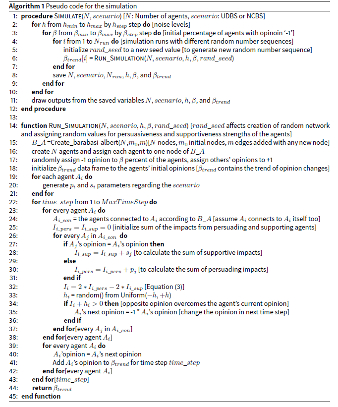
Algorithm 1 describes more details of the simulation. The outputs of the simulation for input values of the parameters \(h\) and initial \(\beta\) are generated by running the simulation for \(N_{run}\) times with different sequences of random numbers, and then the output diagrams and required statistics for \(\beta\) from the first time step until \(MaxTimeStep\) are reported.
The simulation scenarios differ in the assignment of persuasiveness and supportiveness strengths to the agents. In `uniform distribution based strength' (UDBS) scenario the strengths are assigned to the agents using a uniform distribution random variable as depicted in the original model, but in node centrality based strength' (NCBS) scenario, the strengths are assigned to the agents using the agents' centrality in the interaction network and interpreted as their social power. The following subsections describe more details on both scenarios.
Uniform distribution based strengths (UDBS) scenario
In the uniform distribution based strengths (UDBS) scenario, the agents interact according to the proposed model described in Section 3. The persuasiveness power and supportiveness power are both assigned using uniform distribution random functions Uniform(\(0, p_{max}\)) and Uniform(\(0, s_{max}\)), respectively.
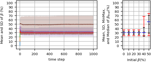
Figure 3 reports changes of \(\beta\), the percentages of agents with the opinion `-1', for an extreme level with no noise, \(h=0\). The right diagram shows statistics of \(\beta_{final}\) against initial \(\beta\). Every circle marker in this diagram shows the mean value of \(\beta_{final}\) for \(N_{run}\) simulation replications. The corresponding standard deviation, min-max values, and median are shown as black bars, red bars, and blue bars, respectively. Every diagram at the left side shows the means and (shaded) standard deviations of \(\beta\) during simulation time steps from the initial state to \(MaxTimeStep\). When the simulation starts from an initial consensus, \(\beta=0\%\), the simulation equilibrium is absolutely the same because there is no opposite pressure and no stochastic behavior to change any opinion during the simulation run. For other initial \(\beta\)s except 50% (e.g., 10%, 20%, 30%, 40%), the final percentage is either frozen majority or orderly fluctuated majority. For these initial \(\beta\)s which are the percentage of minority agents, \(\beta_{final}\) becomes smaller at the equilibrium. In other words, the initial dominant opinion group attracts some agents from the minority opinion group; therefore, there is a tendency toward the dominant opinion group. As discussed in (Hołyst et al. 2000), if the network is complete, consensus will be formed at zero noise level, but in our configuration with scale-free network, the segregation phenomenon, introduced in Section 2, causes no consensus for \(\beta>0\). Starting the simulation from \(\beta=50\%\), mean of \(\beta_{final}\) remains at about 50% at equilibrium. More details on \(\beta=50\%\) will be discussed later in this section.
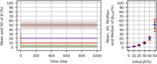
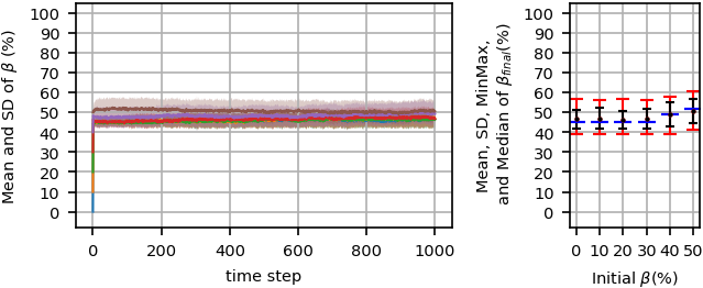
Figure 4 shows the result of another set of simulation runs with the same input parameters as for Figure 3, but the noise level is equal to \(200\), \(h=200\). Again the total behavior of the system is similar to Figure 3, but even starting from consensus, \(\beta=0%\), the system may reach a \(\beta_{final}>0\). Indeed, there is a minimum value for the mean value of \(\beta_{final}\) (about 2%) that starting from \(\beta\)s less than 50% the system converges to that \(\beta_{final}\) on average in equilibrium. Very briefly, starting from \(\beta\le40\%\), the system reaches to a stronger (more probably frozen or orderly fluctuated than non-orderly fluctuated) majority phase in equilibrium.
For \(\beta=50%\), the figure indicates a high standard deviation and a high difference between the minimum and maximum \(\beta\)s because as shown in Figure 8 and will be more discussed later, every simulation replication reaches to the majority of one of both opinion groups in equilibrium with the same probability (\(0.5\)).
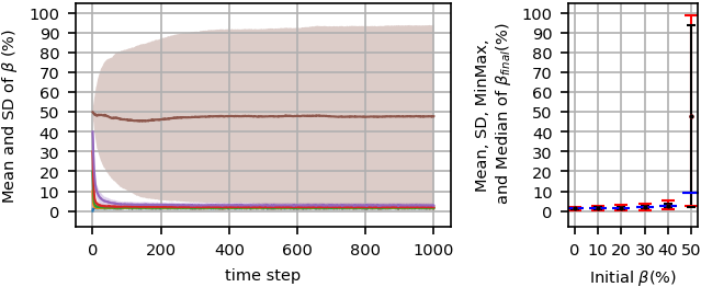
Increasing the noise level to \(600\) (Figure 5) causes forming a non-orderly fluctuated majority phase with \(\beta_{final}\approx30\%\) on average for \(\beta\le40\%\). Comparing Figure Figure 5 with Figure Figure 4 for \(h=200\) reveals that weaker majority phases with higher standard deviations and higher min-max ranges are formed in equilibrium when \(h\) increases to \(600\). When the noise level increases to \(1000\) (Figure 6), a (non-orderly fluctuated) non-majority phase forms in equilibrium for every initial \(\beta\), in which \(\beta_{final}\approx50\%\). Further increasing noise level to \(2000\) (Figure 7), similarly causes non-majority phase, but with lower standard deviations and lower min-max ranges.
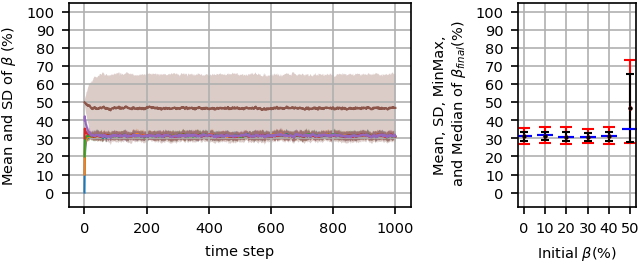
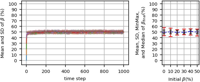

Figure 8 details the system behavior during simulation time steps starting from \(\beta=50%\) in different noise levels. Each curve shows \(\beta\) values for each simulation replication during simulation time steps. As the figure shows, (non-orderly fluctuated) non-majority phase is formed for high enough noise levels, \(h\ge1000\), and the main difference is the dispersion of curves for \(h=1000\) and \(h=2000\). For lower noise level, \(h=600\), a (non-orderly fluctuated) majority phase is formed, where about \(30%\) of the agents fall in the minority group, and the others fall in the majority group. A similar majority phase occurs for \(h=400\) with about \(13%\) of the agents in the minority group, and for \(h=200\) with about 2% of the agents in the minority group. For the last case with no noise, \(h=0\), as the figure presents, more probably frozen majority or orderly fluctuated majority phases (thicker curves) occur in equilibrium, and in some rare cases, frozen non-majority phase or orderly fluctuated non-majority phase (fluctuating around \(\beta=50%\)) may also occur.
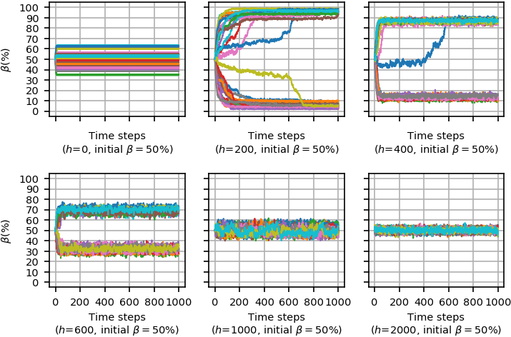
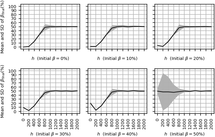
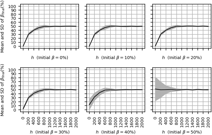
Figure 9 shows another view on the simulation results in which the mean and (shaded) standard deviation of \(\beta_{final}\) for various initial \(\beta\) are shown in separate diagrams. Every diagram shows \(\beta_{final}\) for various noise levels, \(h\), from \(0\) to \(2000\). As the figure shows, for noise levels above a specific value (about \(1000\)), the system equilibrium phase is non-majority for every initial \(\beta\). The figure also shows a non-monotonic trend of the curves for \(\beta=20%, 30%\), and \(40%\), which shows a descending trend of minority (stronger majority) while the noise level increases from zero to \(200\). Afterward, while the noise level increases more, the ascending trend of the curve is observed, thus minority increases (weaker majority). This trend continues until a noise level, where a non-majority phase is formed. The segregation phenomenon, introduced in Section 2, justifies the non-monotonic trend of these curves.
Node centrality based strength (NCBS) scenario
In the `node centrality based strength' (NCBS) scenario, a configuration similar to the UDBS scenario has been used, but the initial assignment of the agents' persuasiveness and supportiveness strengths is proportional to the agents' social power (Friedkin 1986). As discussed in `Persuasion and social power' subsection of Section 2, node degree is a reasonable estimation of social power. Therefore, we define social power for agent \(i\) based on its degree ratio as \(SP_i = \text{d}(i) / \Delta\), where \(\text{d}(i)\) denotes degree of node \(i\) in the network and \(\Delta\) denotes the maximum degree of the nodes in the network, used for normalization. Since the node degrees of Barabási-Albert Network follows a power law distribution, the persuasiveness and supportiveness strengths of the agents are initialized by a power law distribution proportional to the node degrees. This power law distribution is compatible with the final social power distribution studied by the simulation reported in (Lu et al. 2015). Therefore, in this scenario any agent \(i\) is initialized to proportional persuasiveness strength \(p'_i\) in the range \((0, p_{max}]\) and proportional supportiveness strength \(s'_i\) in the range \((0, s_{max}]\) according to Equation 4 and Equation 5, respectively:
| $$p'_i=\frac{\text{d}(i)}{\Delta}p_{max},$$ | (4) |
| $$s'_i=\frac{\text{d}(i)}{\Delta}s_{max}.$$ | (5) |
Substituting \(p_i\) and \(s_i\) with \(p'_i\) and \(s'_i\) respectively in Equation 3 we have Equation 6 for computing \(I_i\) in this scenario:
| $$I_i = \left[\sum_{j \mid o_j \neq o_i} 2 \frac{\text{d}(j)}{\Delta}p_{max} \right] - \left[ \sum_{j \mid o_j = o_i} 2 \frac{\text{d}(j)}{\Delta} s_{max} \right].$$ | (6) |
Figure 10 reports the simulation results for \(h=0\). Comparing this figure with the corresponding figure in the previous scenario (Figure 3), \(\beta\)s have higher standard deviations and wider min-max ranges for an initial \(\beta\ge20\). Furthermore, considering the values of means and medians for \(\beta=20\%, 30\%, 40\%\) shows a positive skewness in the distributions of \(\beta_{final}\), which is related to the power law distribution of the agents' persuasiveness and supportiveness strengths as well as their connectivity. Indeed, there are a few high influential agents with high connectivities and many agents with low strengths and low connectivities in the network. Therefore, in some cases depending on the initial random assignments of opinions to the agents, a relatively high strength may be generated by some hubs with minority opinion, and causes less shrink of minority opinion, or even for \(\beta=40\%\), as min-max bar shows, \(\beta_{final}\) becomes greater than the initial \(\beta\). This phenomenon happens in some higher noise levels as the mean and min-max statistics of \(\beta_{final}\) similarly shows. Figure 10 also reveals that any \(\beta_{final}\) between \(0\%\) and \(100\%\) for \(\beta=50\%\) is possible because the probability of the initial configurations regarding both opinion groups are the same; therefore, majority phases happens with the same probability in both possible opinion groups. However, in some rare cases, a non-majority phase may occur because of partitioning the agents into two equal-size opinion groups.
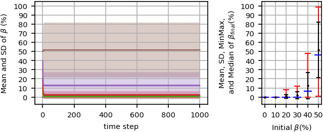
Figure 11 shows system behavior when the noise level increases to \(200\). This noise level causes a non-majority phase in equilibrium for \(\beta\le40%\). For \(\beta\le30%\) the system reaches a non-majority phase with expected \(\beta_{final}\approx30%\), which could be interpreted that the noise level is high enough that the expected value of \(\beta_{final}\) is at least about 30% regardless of initial \(\beta\). As min-max bars show, starting from \(\beta=30%\) or \(\beta=40%\) may result in a majority phase with \(\beta_{final}\) greater than the initial \(\beta\), which could be interpreted as for \(\beta=40%\) in Figure 10.
The noise level more dominates the system behavior when increases to higher levels. Increasing noise level to \(600\) (Figure 12) causes forming a weaker majority (higher percentage for minority opinion); therefore, comparing with (Figure 11) , for \(\beta\le30%\) the system reaches to a higher expected value of \(\beta_{final}\approx46%\) due to the dominance of stochastic behavior of the system on its deterministic behavior.
The system behavior for \(h=1000\) and \(h=2000\) are shown in Figure 13 and Figure Figure 14, respectively. The equilibrium phase for both \(h=1000\) and \(h=2000\) are (non-orderly fluctuated) non-majority phase for all initial \(\beta\)s; however, in equilibrium, the standard deviation for \(h=2000\) is less than the standard deviation for \(h=1000\).
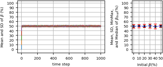
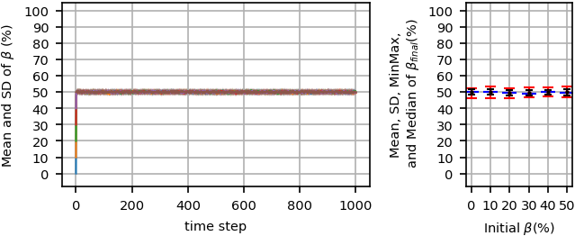
Figure 15 details the system behavior during simulation time steps starting from \(\beta=50%\) in different noise levels. The figure reveals that (non-orderly fluctuated) non-majority phase is formed for high enough noise levels, \(h\ge600\), and the higher noise levels cause a lower standard deviation for \(\beta_{final}\). For the lower noise level, \(h=400\), (non-orderly fluctuated) majority phase is formed, where about \(40%\) of the agents fall in the minority group and the others in the majority group. For \(h=200\), a majority phase forms dividing the agents into about \(30%\) and \(70%\) groups on average. For the last case with no noise, \(h=0\), as the figure shows, similar to UDBS, more probably frozen majority or orderly fluctuated majority phases occur, and in some rarely cases, frozen non-majority or orderly fluctuated non-majority (fluctuating around \(\beta=50%\)) phases are possible. The range of possible \(\beta_{final}\) is wider in this scenario.
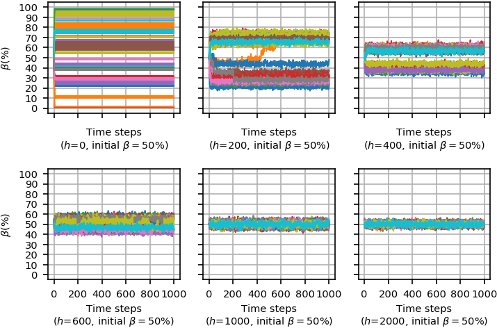
Figure 16 shows the mean and standard deviation of \(\beta_{final}\) for each initial \(\beta\) in various noise levels, from \(0\) to \(2000\). As the figure shows, for noise levels above a specific value (about \(800\)), the system equilibrium phase is non-majority for every initial \(\beta\). In this scenario, unlike the previous one, the trend of the curves for all \(\beta\)s are monotonic because it is more probable that the segregated groups break up due to the presence of a few more influential agents with high connectivity in the network.
Analysis and Discussion
In this section, the experimental results of running the simulation scenarios expressed in the previous section are discussed and statistically analyzed.
Analysis of the UDBS scenario
From the viewpoint of any agent \(i\), the agents of the system could be partitioned into two disjoint sets including the disagreed agents and agreed agents. Equation 3 could be rewritten as:
| $$I_i = \sum_{j=1}^{N_d} 2p_j - \sum_{j=1}^{N_a} 2s_j, $$ | (7) |
In the UDBS scenario, both \(p_j\) and \(s_j\) are random variables with uniform distributions Uniform\((0, p_{max})\) and Uniform\((0, s_{max})\) respectively. Since \(p_{max}=s_{max}\), we suppose \(c\) as \(c = p_{max}=s_{max}\); therefore,
| $$p_j = s_j = \text{Uniform}(0,c),$$ | (8) |
| $$\mu_{p_j} = \mu_{s_j} = \frac{c}{2},$$ | (9) |
| $$\sigma_{p_j}^2 = \sigma_{s_j}^2 = \frac{c^2}{12}.$$ | (10) |
Since \(I_i\) is a linear combination of random variables \(p_j\) and \(s_j\), from Equation 7 and Equation 9 we have the mean value of \(I_i\) as:
| $$\mu_{I_i} = 2N_d(\frac{c}{2}) - 2N_a(\frac{c}{2}).$$ | (11) |
The parameter \(\beta\) in the simulation determines the percentage of the agents with opinion `-1'. Starting the simulation with \(\beta\), without loss of generality, we suppose agent \(i\) is an agent whose initial opinion is `-1', therefore, \(\beta\) percent of all the agents are initialized to opinions agreed with agent \(i\), and \((1-\beta)\) of the agents are initialized to the other opinion. Since our network is a Barabási-Albert network with \(m\) edges for any newly added node during network generation, any node is connected to \(2m\) nodes on average (Barabási & Albert 1999). Therefore, it is expected that agent \(i\) is connected on average to \(2m(1-\beta)\) disagreed agents and \(2m\beta\) agreed agents (including itself). Substituting \(2m(1-\beta)\) and \(2m\beta\) for \(N_d\) and \(N_a\) respectively in Equation 11, \(\mu_{I_i}\) is calculated as:
| $$\mu_{I_i} = 2N_d(\frac{c}{2}) - 2N_a(\frac{c}{2}).$$ | (12) |
| $$\mu_{I_i} = 2m(1-2\beta)c.$$ | (13) |
Using Equation 12 for the variance of \(p_j\) and \(s_j\), and Equation 2 for the linear combination of \(p_j\) and \(s_j\) to generate \(I_i\), the variance of \(I_i\), \(\sigma_{I_i}^2\), is calculated as:
| $$\sigma_{I_i}^2 = \sum_{j=1}^{2m(1-\beta)}2^2\sigma_{p_j}^2 + \sum_{j=1}^{2m(\beta)}2^2\sigma_{s_j}^2 = \frac{2m}{3}c^2,$$ | (14) |
| $$\sigma_{I_i} = \sqrt{\frac{2m}{3}}c.$$ | (15) |
From Equation 12 for the mean value of \(I_i\), it is clear that if \(\beta=50\%\), i.e., the first impression is in such a way that the sizes of both opinion groups are the same, the expected value of \(I_i\) becomes zero. Since the expected value of noise level \(h\) equals zero, the expected value of the argument of sign function in Equation 2 becomes zero as well; therefore \(o_i\) in the next time step is undetermined. Thus the probabilities for agents to stay/change their opinions are the same (\(0.5\)). Consequently, depending on the random assignments of persuasiveness and supportiveness strengths to the agents as well as the topology of the random network, the system goes toward a majority phase with one of the possible opinions with equal probability in equilibrium (Figure 8), and in some rare cases, the system may remain in non-majority phase (frozen or orderly-fluctuated).
From Equation 12 it is expected that if \(\beta<50\%\) then we have \(I_i>0\); therefore it is more probable that the agents in the minor group change their opinions to the majority's opinion. The trend of changing some agents' opinion from minority group to majority group stops after some time steps due to segregation phenomenon.
Our connection network is generated by Barabási-Albert algorithm; thus node degrees follow a power law distribution with exponent \(\gamma \le 3\), and as discussed in (Bianconi & Marsili 2006), contains a relatively huge number of small loops. These small loops make a lot of segregated agents in the network that don't change their opinions at zero noise level. Thus, for zero noise level, as Figure 3 shows, starting from any \(\beta<50\%\), results in \(0<\beta_{final}<\beta\) in equilibrium.
By increasing the noise level, some of the members of the segregated groups change their opinions because of their more stochastic behavior. Therefore, when one or more agents change their opinions, this may inevitably lead other members of the segregated group to switch to the other opinion; therefore, initial \(\beta\) becomes more important to determine \(\beta_{final}\). This segregation phenomenon expresses why in Figure 9 when the noise level increases from zero to \(200\), the mean value of \(\beta_{final}\) becomes lower for initial \(\beta\) equal to \(20\%\), \(30\%\), or \(40\%\).
Increasing the noise level to enough values leads the system trend toward non-majority phase in which about half of the agents have one of the two possible opinions at the end of the simulation run. To analyze this phenomenon, without loss of generality we focus on the agents with opinion `-1' and rewrite Equation 2 as:
| $$o_i(t+1) = \text{sign}[I_i(t)-h_i].$$ | (16) |
Now we regard \((I_i(t)-h_i)\) as a new random variable composed of two independent random variables \(I_i(t)\) and \(h_i\). Since \(h_i\) is a random variable with the distribution Uniform\((-h, +h)\), we have \(\mu_{h_i}=0\). Thus the mean value of \(I_i(t)\) with noise level, \((I_i(t)-h_i)\), is the same as Equation 12. But for the variance of \((I_i(t)-h_i)\) using Equation 13 we have:
| $$\sigma_{I_i-h_i}^2 = \frac{2}{3}mc^2+\frac{(h-(-h))^2}{12}= \frac{2}{3}mc^2+\frac{h^2}{3},$$ | (17) |
Analysis of the NCBS scenario
In the NCBS scenario, \(p_i\) and \(s_i\) are proportional to social power according to Equation 4 and Equation 5. Substituting \(c\) for \(p_{max}\) and \(s_{max}\), equation for \(p'_i\) and \(s'_i\) could be written as:
| $$p'_i = s'_i = \frac{\text{d}(j)}{\Delta}c,$$ | (18) |
For \(I_i\), similar to Equation 7, we have
| $$I_i = \sum_{j=1}^{N_d} 2p'_j - \sum_{j=1}^{N_a} 2s'_j,$$ | (19) |
| $$I_i = \frac{2}{\Delta} \left(\sum_{j=1}^{N_d} \text{d}(j) - \sum_{j=1}^{N_a} \text{d}(j) \right) c,$$ | (20) |
Since the mean value of node degrees in Barabási-Albert network is \(2m\), the mean value of \(I_i\) which is a linear combination of random variables \(\text{d}(j)\) is calculated from Equation 19 as:
| $$\mu_{I_i} = \frac{2}{\Delta} (2m)(1-2\beta) (2m) c.$$ | (21) |
Comparing Equation 12 for \(\mu_{I_i}\) in the UDBS scenarios and Equation 20 for \(\mu_{I_i}\) in the NCBS scenarios we have:
| $$\mu_{I_i(NCBS)} = \frac{4m}{\Delta} \mu_{I_i(UDBS)},$$ | (22) |
Therefore:
| $$|\mu_{I_i(NCBS)}| \ll |\mu_{I_i(UDBS)}|.$$ | (23) |
Equation 22 implies that with the same configuration for both scenarios, since \(I_i\) is much closer to zero in the NCBS scenario, the stochastic behavior because of the noise level more dominates the deterministic behavior comparing with the UDBS scenario.
Another important point to compare the dynamics of both scenarios is comparing the variance of \(I_i\) in the scenarios. The probability distribution of node degrees, \({d}(j)\), in Barabási-Albert network is power law \(P(k) \sim k^{-\gamma}\) where \(\gamma=2.9\pm0.1\) (Barabási & Albert 1999). The standard deviation of the power law distribution is theoretically calculated as:
| $$\sigma = \frac{\gamma - 1}{\gamma - 3} k_{min}^2,$$ | (24) |
Thus, for \(\gamma \le 3\) variance does not exist or is infinite theoretically. Therefore, this high variance plus the variance imposed by the noise level leads the system to have a more tendency toward non-majority phase compared to the UDBS scenario, as comparing Figure 9 with 16 clarifies.
It is also notable that due to the higher variance of persuasiveness and supportiveness strengths of the agents in the NCBS scenario, the probability of segregation is much lower comparing with the UDBS scenario, and as Figure 16 shows, leads the system to approach monotonically to non-majority phase when the noise level increases. For high enough noise level, the system phase changes to non-majority very similar to the UDBS scenario, but the higher variance of persuasiveness and supportiveness strengths in the NCBS scenario leads the corresponding noise level to be lowered.
Conclusion
Power law distributions have been found in many natural and social phenomena, and simulations of social phenomena based on this distribution are more realistic in many cases. We have investigated the social impact model of opinion formation (Hołyst et al. 2001; Latané 1981) in Barabási-Albert interaction networks with power law distribution of node degrees (Barabási & Albert 1999). In the social impact model of opinion formation, in every time step, any individual/agent is affected by others to change or persist in his current opinion. Every agent is characterized by persuasiveness and supportiveness strengths which are initialized using a uniform probability distribution. We have considered two scenarios in this research based on the distribution of the agents' persuasiveness and supportiveness strengths: uniform distribution based strengths (UDBS) based on a uniform distribution, as in the original model; and node centrality based strengths (NCBS) based on a power law distribution proportional to the agents' centrality in their network. The latter scenario is based on some studies that show individuals' centralities are positively related to their ability to influence others (Yoo & Alavi 2004; Huffaker 2010; Weeks et al. 2017; Noelle-Neumann 1983; Weimann et al. 2007; Baym 2000).
The social impact model also has a noise parameter, indicating the individual's inexplicable opinion changes due to any other influential factors, such as public media, affects, and emotions. The noise levels affect the system phase transition, and in this research, we considered the role of noise levels in phase transition in both mentioned scenarios of the model. Two phases are possible in equilibrium: majority and non-majority; and in each one, the possible cases are: frozen, orderly fluctuated, and non-orderly fluctuated. The consensus is a special case of majority phase. The segregation phenomenon, which often emerges in human societies when two or more well-connected sub-networks exist with a few connections to the nodes out of the sub-network (Zanette & Gil 2006; Shi et al. 2013; Feliciani et al. 2017), also plays a key role in opinion phase transitions.
We investigated by agent-based simulations and analytical considerations in both scenarios, how opinion phases are formed in equilibrium considering the noise level and various initial population size of agents in both opinion groups. The results of increasing noise level are summarized as follows:
- At zero noise level, the system behavior is fully deterministic. Starting from the consensus, the system stays in the consensus forever. In the UDBS, starting from a majority results in a relatively stronger majority for all the initial combinations of opinion group sizes. In NCBS scenario, although starting from a majority results in a majority, for some initial combinations of opinion groups a weaker majority forms in equilibrium. Indeed, in these cases, the few high influential agents with high connectivity in the scale-free network have the same minority opinion and act as strong leaders in the society; therefore, the population of the minority group increases in equilibrium.
- Increasing the noise level breaks some segregation groups and depending on the noise level, a minimum value for the mean value of minority group population is observed. This minimum value for NCBS is higher than the corresponding value for UDBS scenario. In NCBS scenario, for some combinations of the initial population of the opinion groups, the minority group may become the majority group in equilibrium, which is the consequence of the presence of few strong leaders in the minority opinion group.
- In high enough noise levels, the social system reaches a non-majority in both scenarios regardless of the initial population of opinion groups due to the dominance of stochastic behavior of the system on its deterministic behavior. This high enough noise level for NCBS scenario is lower comparing with UDBS scenario.
The increase in the noise level from zero in UDBS scenario may cause a non-monotonic trend of the minority population in equilibrium due to the segregation phenomenon. However, in NCBS scenario, segregated groups are more easily broken due to the presence of strong leaders with high connectivities, and consequences the monotonic increase of minority population in equilibrium.
Starting from two equal size opinion groups, in zero or low noise levels, one of the opinion groups becomes majority group with the equal probabilities in equilibrium; and for high enough noise levels, similar to the other initial combinations, non-majority phase forms in equilibrium.
Although this research is a step toward a better understanding of the social opinion dynamics, some more studies are needed to complete it. We estimated the social power of persuading others with the same power law distribution of node degrees in the network. This social power has been estimated by power law distributions in some other researches as well, but some more in-depth studies with real world data and case studies are required to estimate it more precisely and refine our assumption considering other parameters. For example, individuals have different resistance to persuasion and opinion change across topics, sources, situations, and so on (Briñol et al. 2004, Chapter 5). Furthermore, in many cases, affects and emotions are influential factors in persuasion. According to ELM (Petty & Cacioppo 1986), when people are unwilling or unable to analyze received information, for example, it is low in personal relevance or there are many distractions, variables such as a person's emotional state have an impact on attitudes; therefore, running a relatively simple and low effort process such as forming a direct relationship between the feeling state and the opinion is expected.
Model Documentation
The model is implemented in Python programming using the agent-based modeling framework MESA. The code and necessary documents are available online here: https://www.comses.net/codebase-release/2f3d7e0b-1942-422e-895c-61989d9ab99f/.References
ABELSON, R. P. (1964). Mathematical models of the distribution of attitudes under controversy. Contributions to Mathematical Psychology.
AFSHAR, M. & Asadpour, M. (2010). Opinion formation by informed agents. Journal of Artificial Societies and Social Simulation, 13(4), 5: https://www.jasss.org/13/4/5.html. [doi:10.18564/jasss.1665]
AJZEN, I. (1992). Persuasive communication theory in social psychology: A historical perspective. In Influencing Human Behavior Theory and Applications in Recreation and Tourism Natural Resources, (pp. 1–27). Urbana, IL: Sagamore.
ALBI, G., Pareschi, L., Toscani, G. & Zanella, M. (2017). Recent advances in opinion modeling: control and social influence. In Active Particles, Volume 1, (pp. 49–98). Berlin/Heidelberg: Springer. [doi:10.1007/978-3-319-49996-3_2]
ALEKSIEJUK, A., Hoyyst, J. A & Stauffer, D. (2002). Ferromagnetic phase transition in Barabasi-Albert networks. Physica A: Statistical Mechanics and its Applications, 310(1-2), 260-266. [doi:10.1016/s0378-4371(02)00740-9]
ARAL, S., & Walker, D. (2012). Identifying influential and susceptible members of social networks. Science, 337(6092), 337-341. [doi:10.1126/science.1215842]
AXELROD, R. (1997). The Complexity of Cooperation: Agent-Based Models of Competition and Collaboration. Princeton, NJ: Princeton University Press.
BARABÁSI, A.-L. (2009). Scale-free networks: a decade and beyond. Science, 325(5939), 412–413. [doi:10.1126/science.1173299]
BARABÁSI, A.-L. & Albert, R. (1999). Emergence of scaling in random networks. Science, 286(5439), 509–512. [doi:10.1126/science.286.5439.509]
BARRAT, A., Barthelemy, M. & Vespignani, A. (2008). Dynamical Processes on Complex Networks. Cambridge, MA: Cambridge University Press.
BAYM, N. K. (2000). Tune In, Log On: Soaps, Fandom, and Online Community (Vol. 3). London, UK: Sage.
BIANCHI, F. & Squazzoni, F. (2015). Agent-based models in sociology. Wiley Interdisciplinary Reviews: Computational Statistics, 7(4), 284–306. [doi:10.1002/wics.1356]
BIANCONI, G. & Marsili, M. (2006). Number of cliques in random scale-free network ensembles. Physica D: Non-linear Phenomena, 224(1-2), 1–6. [doi:10.1016/j.physd.2006.09.013]
BINDER, K. (1987). Theory of first-order phase transitions. Reports on Progress in Physics, 50(7), 783. [doi:10.1088/0034-4885/50/7/001]
BRIÑOL, P., Rucker, D. D., Tormala, Z. L. & Petty, R. E. (2004). 'Individual differences in resistance to persuasion: The role of beliefs and meta-beliefs.' In E. S. Knowles & J. A. Linn (Eds.), Resistance and Persuasion, (p. 83). Mahwah, NJ: Lawrence Erlbaum Associates.
CASTELLANO, C., Fortunato, S. & Loreto, V. (2009). Statistical physics of social dynamics. Reviews of Modern Physics, 81(2), 591. [doi:10.1103/revmodphys.81.591]
CHACOMA, A. & Zanette, D. H. (2015). Opinion formation by social influence: From experiments to modeling. PLoS ONE, 10(10), e0140406. [doi:10.1371/journal.pone.0140406]
CHATTOE-BROWN, E. (2013). Why sociology should use agent based modelling. Sociological Research Online, 18(3), 1–11. [doi:10.5153/sro.3055]
DEFFUANT, G., Neau, D., Amblard, F. & Weisbuch, G. (2000). Mixing beliefs among interacting agents. Advances in Complex Systems, 3(01n04), 87–98. [doi:10.1142/s0219525900000078]
DEGROOT, M. H. (1974). Reaching a consensus. Journal of the American Statistical Association, 69(345), 118–121 [doi:10.1080/01621459.1974.10480137]
DEMARZO, P. M., Vayanos, D., & Zwiebel, J. (2003). Persuasion bias, social influence, and unidimensional opinions. The Quarterly Journal of Economics, 118(3), 909-968. [doi:10.1162/00335530360698469]
JUN, D. & Da-Ren, H. (2007). Phase Transition of a Distance–Dependent Ising Model on the Barabasi–Albert Network. Chinese Physics Letters, 24(12), 3355. [doi:10.1088/0256-307x/24/12/018]
DURKHEIM, E. (1997 [1893]). The Division of Labor in Society. New York: The Free Press.
ELTAYEBY, O., Molnar, P. & George, R. (2014). Measuring the influence of mass media on opinion segregation through twitter. Procedia Computer Science, 36, 152–159. [doi:10.1016/j.procs.2014.09.062]
ERCHUL, W. P. & Raven, B. H. (1997). Social power in school consultation: A contemporary view of french and raven’s bases of power model. Journal of School Psychology, 35(2), 137–171. [doi:10.1016/s0022-4405(97)00002-2]
FELICIANI, T., Flache, A. & Tolsma, J. (2017). How, when and where can spatial segregation induce opinion polarization? Two competing models. Journal of Artificial Societies and Social Simulation, 20(2), 6: https://www.jasss.org/20/2/6.html. [doi:10.18564/jasss.3419]
FESTINGER, L. (1957). A Theory of Cognitive Dissonance, vol. 2. Palo Alto, CA: Stanford University Press
FRENCH Jr, J. R. P. (1956). A formal theory of social power. Psychological Review, 63(3), 181.
FRIEDKIN, N. E. (1986). A formal theory of social power. Journal of Mathematical Sociology, 12(2), 103–126.
FRIEDKIN, N. E. & Johnsen, E. C. (1990). Social influence and opinions. Journal of Mathematical Sociology, 15(3-4), 193–206. [doi:10.1080/0022250x.1990.9990069]
FRIENDKIN, N. & Johnsen, E. (1999). Social influence networks and opinion change. Adv Group Proc, 16, 1–29.
FRONCZAK, P., Fronczak, A. & Hołyst, J. A. (2007). Phase transitions in social networks. The European Physical Journal B, 59(1), 133–139 [doi:10.1140/epjb/e2007-00270-8]
HAUKE, J., Lorscheid, I. & Meyer, M. (2017). Recent development of social simulation as reflected in JASSS between 2008 and 2014: A citation and co-citation analysis. Journal of Artificial Societies and Social Simulation, 20(1), 5: https://www.jasss.org/20/1/5.html. [doi:10.18564/jasss.3238]
HEGSELMANN, R., & Krause, U. (2002). Opinion dynamics and bounded confidence models, analysis, and simulation. Journal of Artificial Societies and Social Simulation, 5(3), 2: https://www.jasss.org/5/3/2.html.
HINZ, O., Skiera, B., Barrot, C. & Becker, J. U. (2011). Seeding strategies for viral marketing: An empirical comparison. Journal of Marketing, 75(6), 55–71. [doi:10.1509/jm.10.0088]
HOŁYST, J. A., Kacperski, K. & Schweitzer, F. (2000). Phase transitions in social impact models of opinion formation. Physica A: Statistical Mechanics and its Applications, 285(1-2), 199–210. [doi:10.1016/s0378-4371(00)00282-x]
HOŁYST, J. A., Kacperski, K. & Schweitzer, F. (2001). Social impact models of opinion dynamics. In Annual Reviews Of Computational PhysicsIX, (pp. 253–273). World Scientific. [doi:10.1142/9789812811578_0005]
HOVLAND, L. A. A., Carl Iver & Sheuield, F. D. (1949). Experiments on Mass Communication. Princeton, NJ: Princeton University Press.
HU, H. (2017). Competing opinion diffusion on social networks. Royal Society Open Science, 4(11), 171160. [doi:10.1098/rsos.171160]
HUFFAKER, D. (2010). Dimensions of leadership and social influence in online communities. Human Communication Research, 36(4), 593–617. [doi:10.1111/j.1468-2958.2010.01390.x]
IYENGAR, R., Van den Bulte, C. & Valente, T. W. (2011). Opinion leadership and social contagion in new product diffusion. Marketing Science, 30(2), 195–212. [doi:10.1287/mksc.1100.0566]
JALILI, M. (2013). Social power and opinion formation in complex networks. Physica A: Statistical mechanics and its applications, 392(4), 959–966. [doi:10.1016/j.physa.2012.10.013]
KADANOU, L. P. (2009). More is the same; phase transitions and mean field theories. Journal of Statistical Physics, 137(5-6), 777.
KATZ, E. (1957). The two-step flow of communication: An up-to-date report on a hypothesis. Public Opinion Quarterly, 21(1), 61–78. [doi:10.1086/266687]
KLEMM, K., Eguiluz, V. M., Toral, R. & Miguel, M. S. (2002). Cultural transmission and optimization dynamics. arXiv preprint cond-mat/0210173.
KLEMM, K., Eguíluz, V. M., Toral, R. & San Miguel, M. (2003). Nonequilibrium transitions in complex networks: A model of social interaction. Physical Review E, 67(2), 026120. [doi:10.1103/physreve.67.026120]
KURAHASHI-NAKAMURA, T., Mäs, M. & Lorenz, J. (2016). Robust clustering in generalized bounded confidence models. Journal of Artificial Societies and Social Simulation, 19(4), 7: https://www.jasss.org/19/4/7.html.. [doi:10.18564/jasss.3220]
LASWELL, H. D. (1948). The structure and function of communication in society. New York: The Institute for Religious and Social Studies.
LATANÉ, B. (1981). The psychology of social impact. American Psychologist, 36(4), 343.
LEVY, M. (2005). Social phase transitions. Journal of Economic Behavior & Organization, 57(1), 71–87.
LIANG, H., Dong, Y. & Li, C. (2016). Dynamics of uncertain opinion formation: An agent-based simulation. Journal of Artificial Societies and Social Simulation, 19(4), 1: https://www.jasss.org/19/4/1.html.. [doi:10.18564/jasss.3111]
LIU, B. & Zhang, L. (2012). A survey of opinion mining and sentiment analysis. In Mining Text Data (pp. 415-463). Springer, Boston, MA. [doi:10.1007/978-1-4614-3223-4_13]
LU, X., Mo, H. & Deng, Y. (2015). An evidential opinion dynamics model based on heterogeneous social influential power. Chaos, Solitons & Fractals, 73, 98–107. [doi:10.1016/j.chaos.2015.01.007]
MACAL, C. & North, M. (2014). Introductory tutorial: Agent-based modeling and simulation. In Proceedings of the Winter Simulation Conference 2014, (pp. 6–20). IEEE. [doi:10.1109/wsc.2014.7019874]
MACY, M. & Tsvetkova, M. (2015). The signal importance of noise. Sociological Methods & Research, 44(2), 306–328. [doi:10.1177/0049124113508093]
MÄS, M., Flache, A. & Helbing, D. (2010). Individualization as driving force of clustering phenomena in humans. PLoS computational biology, 6(10), e1000959. [doi:10.1371/journal.pcbi.1000959]
NOELLE-NEUMANN, E. (1983). Spiegel Dokumentation: Persönlichkeitsstärke. Hamburg: Spiegel Verlag.
PERC, M. (2016). Phase transitions in models of human cooperation. Physics Letters A, 380(36), 2803–2808. [doi:10.1016/j.physleta.2016.06.017]
PETTY, R. E. (2018). Attitudes and Persuasion: Classic and Contemporary Approaches. London, UK: Routledge.
PETTY, R. E. & Cacioppo, J. T. (1986). The elaboration likelihood model of persuasion. In Communication and Persuasion, (pp. 1–24). Springer, New York, NY. [doi:10.1007/978-1-4612-4964-1_1]
PINEDA, M., Toral, R. & Hernandez-Garcia, E. (2009). Noisy continuous-opinion dynamics. Journal of Statistical Mechanics: Theory and Experiment, 2009(08), P08001. [doi:10.1088/1742-5468/2009/08/p08001]
SALEHI, S. & Taghiyareh, F. (2016). The impact of structural position on opinion leadership in social network. International Journal of Information and Communication Technology Research, 8(4), 45–54.
SHI, F., Mucha, P. J. & Durrett, R. (2013). Multiopinion coevolving voter model with infinitely many phase transitions. Physical Review E, 88(6), 062818. [doi:10.1103/physreve.88.062818]
WEEKS, B. E., Ardèvol-Abreu, A. & Gil de Zúñiga, H. (2017). Online influence? social media use, opinion leadership, and political persuasion. International Journal of Public Opinion Research, 29(2), 214–239. [doi:10.1093/ijpor/edv050]
WEIMANN, G., Tustin, D. H., Van Vuuren, D. & Joubert, J. (2007). Looking for opinion leaders: Traditional vs. modern measures in traditional societies. International Journal of Public Opinion Research, 19(2), 173–190. [doi:10.1093/ijpor/edm005]
YOO, Y. & Alavi, M. (2004). Emergent leadership in virtual teams: What do emergent leaders do? Information and Organization, 14(1), 27–58. [doi:10.1016/j.infoandorg.2003.11.001]
ZANETTE, D. H. & Gil, S. (2006). Opinion spreading and agent segregation on evolving networks. Physica D: Nonlinear Phenomena, 224(1-2), 156–165. [doi:10.1016/j.physd.2006.09.010]