
Introduction
Firms have actively participated in developing ICT-based convergent technologies to cope with the diversification of technology demands resulting from the rapid development of ICT technology since the early 2000s (Nordmann 2004; Roco 2007). As a strategy for developing convergent technologies, the importance of collaborations among firms with different innovation capacities has increased (Cho et al. 2015; Nordmann 2004). Collaborative innovations enable firms to (a) respond to rapidly changing technology needs and (b) reduce innovation costs by implementing internal innovations (Williamson 1981). An ecosystem with collaborative innovation can improve efficiency associated with internal innovation by sharing innovation capabilities. Many developed countries have implemented policies to promote the participation of firms in collaborative innovation (Roco 2007).
However, firms do not actively participate in cooperative innovation as much as the governments expect (Leiponen 2002). Some researchers argue that size asymmetry among partners can hinder the formation of strategic alliances (Kogut 1988). Other scholars have claimed that the larger the difference in size between partners, the higher the administrative costs associated with collaboration (Park & Ungson 1997; Kelly, Schaan, & Joncas 2002). In an industry with a polarized firm size distribution, differences in firm size can hinder collaborative innovation.
The rapid growth of the ICT industry in the 2000s caused polarization between large and small enterprises. In many countries, the firm size distribution (FSD) in the ICT industry is known to be highly skewed (Ceausu & Bourbonnais 2014; Henrekson & Johansson 1999; Johansson 2004; KISDI 2007). Gibrat (1931) argued that the FSD in a mature industry has a stable lognormal distribution. Industries in developed countries consist of a small number of large firms and a large number of SMEs and have an FSD with an asymmetrical structure skewed to the right (Axtell 2001). The claim that size heterogeneity appears within the industry has led many researchers to seek patterns of FSD distribution in an industry (Arrighetti, Landini, & Lasagni 2014; Babutsidze 2016; D’Este 2005; Na, Lee, & Baek 2017; Noda & Collis 2001).
Firm size heterogeneity refers to size disparities in the FSD within an industry. Size heterogeneity depends on various economic and technological factors, but it can also affect economic and technological change (Cantner & Hanusch 2001). Some researchers have suggested that heterogeneity in FSD may affect the economic performance of the industry (Lee 2009; Malerba 2005). However, understanding the relationship between size heterogeneity and innovation pattern is primarily based on conceptual discussions (Cantner & Hanusch 2001; Malerba 2005). Therefore, direct evidence for the relationship between the two is lacking.
This study explores how collaborative innovation patterns differ according to the size heterogeneity in FSD. If market-dominant large firms lead innovations, the innovation gap between large firms and SMEs increases (Na et al. 2017; Nelson & Winter 1982), the increase in the level of size heterogeneity can make the relationships between innovation-led firms and the rest of the industry more hierarchical, which can also negatively affect the collaborative innovation between firms.
However, several limitations restrict the empirical analysis. First, although firms regularly interact with one another in an industry, the mechanism of this interaction is hardly known (Yurtseven & Tandoğan 2012). Despite the differences in the factors, mechanisms, and interactions that affect innovation in each industry, there have been insufficient explorations of the industry-level variables that affect innovation. Unlike firm-level research, industry-level research is challenging when attempting to control innovation mechanisms; it is also challenging to find comparable groups that are similar in all conditions and differ only in the FSD in reality. Second, since industry-level data is not standardized by country, it is also challenging to build datasets that contain a sufficient number of industries to have statistical power. Therefore, there are restrictions on setting counterfactuals for econometric analysis.
This study (a) produced counterfactuals in which all the conditions except the FSD are homogeneous, and (b) tried to establish theoretical propositions by comparing their collaborative innovation patterns through simulation experiments. To do so, this study focused on the Korean ICT industry, which is known to have a high level of heterogeneity in FSD. I used agent-based modelling (ABM), which is a proper methodology for modelling dynamic systems in which interactions among agents occur to analyse difficult real-world problems (Tesfatsion 2006). Innovation is a complex process, while ABM can model, explore and analyse the behaviour of heterogeneous agents with various mechanisms that are difficult to explain using mathematical models (Watts & Gilbert 2014). Thanks to these advantages, ABM has been used to analyse the formation of inter-firm networks (Özman 2008), inter-firm relationships (Squazzoni & Boero 2002), and the relationship between size heterogeneity and firm behaviour (Catullo 2013; Richiardi 2004). For instance, Cerulli (2012) explored the effects of R&D funding policies using ABM based on game theory. Angelini et al. (2017) investigated the effects of R&D subsidies and network topologies on innovation performance using network-based ABM. Here, I wanted to contribute to shedding light on the relationship between size heterogeneity and collaborative innovation between firms by illustrating the simple but essential patterns of complex interactions in the innovation ecosystem.
Modeling Collaborative Innovation in the Korean ICT Industry
Context: Korean ICT industry
This study focused on the Korean ICT industry. Korea has one of the most advanced ICT industries in the world, as well as one of the highest levels of ICT infrastructure. The R&D expenditure to GDP ratio is the highest among the OECD countries, indicating that the Korean ICT industry is highly innovation-intensive. Korea has reached the top position in the ICT Development Index (IDI) ranking, which indicates a high level of ICT development in a country (ITU 2016). Despite its short history of industrial development, the Korean ICT industry has innovative firms, such as Samsung and LG, which hold an essential position in the global market.
The Korean ICT industry has its unique features represented by the term "Chaebol" (Steers, Shin, & Ungson 1989). Chaebol refers to family-owned conglomerates consisting of large, individual firms. Korean firms have a hierarchical relationship focused on market-dominant firms (Jung & Hong 2015). Since some large firms have dominated innovation in the Korean ICT industry with high market concentrations, the gap between large firms and SMEs in innovation capacity is increasing in the Korean ICT industry.
Model description
Agents and landscape
I built an agent-based model replicating the Korean ICT industry. To specify agents, I collected firm data from KISVALUE and the annual report published in the Financial Supervisory Service's (FSS) Digital Analysis, Retrieval, and Transfer System[1]. A total of 524 Korean firms were classified as ICT firms defined by the KIS-Industry Classification (KIS-IC). These firms operate in 17 Korean provinces and cities. The firm data included annual sales and location information for Korean ICT firms. Sales distribution data skewed strongly to the right, suggesting a very high FSD (See Figure 4). Location distribution was also concentrated in the metropolitan area, where 74% of the ICT firms were located in the Seoul metropolitan area, including Seoul and Gyeonggi Province. Inter-firm collaborative innovation data were collected from the patent data registered with the Korean Intellectual Property Office published in the National Digital Science Library[2]. The data included all joint patent data among Korean ICT firms from 1980 to 2015 and revealed that 79% of Korean ICT firms had registered patents, but only 12% had joint patents.
Firms had three attributes, which included size, location, and strategy. First, the size distribution of the firms followed the sales distribution of 2015. Second, I used GIS data[3] to make a GIS-based virtual space of 17 provinces and cities; the model was initialized with 524 agents at their address location in South Korea (see Figure 1). Third, firms had unique strategies, and they chose cooperation and defection according to their situation and strategy. I set 64 firms that participated in at least one collaborative innovation during the past 35 years, as of 2015, firms that could potentially behave cooperatively. I assumed that firms were Pavlovian firms. 460 firms that had not participated in collaborative innovation over the past 35 years were set as "defective firms" that were not willing to cooperate. Also, 109 firms that had not performed innovation activities in the last 35 years among the defective firms were classified as non-innovative firms. Non-innovative firms did not engage in innovation activities and, therefore, did not participate in inter-firm interactions. This model included 64 Pavlovian firms and 460 defective firms and the defective firms included 109 non-innovative firms.
In the virtual space, firms interact with each other according to the spatial NIPD game and decide whether to perform collaborative innovation[4]. Participation in collaborative innovation has been actively analysed using game theory since it has been perceived as a process by which firms choose the optimal strategy of collaboration or non-collaboration (Suzumura 1992). Since Axelrod (1984), researchers have modelled collaboration using Iterated Prisoner's Dilemma (IPD) games. Gulati, Khanna & Nohria (1994) suggested that modelling assurance/coordination game with the Prisoner’s dilemma is suitable because inter-firm collaboration, like a strategic alliance, is a social dilemma problem. Moreover, they claim that the Prisoner’s dilemma game is the most popular model for inter-firm collaboration. Similarly, Arend & Seale (2005) argued that the formation of alliances among firms is essentially a prisoner’s dilemma game. Note that many previous studies analysing strategic alliances and collaborative innovations were based on the Prisoner’s dilemma game (Arend & Seale 2005; Axelrod 1997; McMillan, Mauri, & Casey 2014; Yun, Won, & Park 2016).
Not all collaborative innovation studies utilize the same game model, with differences according to the type of innovation in detail. Some studies have used non-cooperative games to analyse spillovers in R&D races (Martin 2002) or Nash bargaining games to analyse collaborative product development (Arsenyan, Büyüközkan, & Feyzioğlu 2015). However, these studies either (a) assumed limited types of collaboration or (b) analysed interactions that were closer to competition rather than collaboration. Researchers have analysed various types of collaborative innovations such as knowledge sharing (Yang & Wu 2008), strategic alliances (Arend 2009; Arend & Seale 2005), open innovations (Yun et al. 2016), and collaborative R&D (Chiang 1995) using IPD or PD games. The model used in the present study was designed to observe changes in collaborative innovation patterns over time. An iterated Prisoner’s dilemma game is the most suitable game model for this study because it focuses on observing the progress of the cooperation over time between innovators. An N-player game is also appropriate to implement interactions among multiple innovators. This study used a “spatial N-person iterated Prisoner’s dilemma (NIPD) game.” There are cases in which an NIPD game is used in strategic collaboration research as well as general cooperation (Arend & Seale 2005; Schweitzer, Behera, & Muhlenbein 2002; Waltman 2011; Yun et al. 2016). I elaborate on the firm’s decision-making process below.
Partner selection
This study used the Huff model (Huff 1964), a probabilistic gravitation model, as a partner selection mechanism. Previous studies have used the gravity model to analyse collaborative innovation (Maggioni & Uberti 2007; Montobbio & Sterzi 2013; Morescalchi et al. 2015; Picci 2010; Scherngell & Barber 2009). Here, the Huff model has been used to determine the probability that two firms will establish a partnership. The equation for the Huff model was as follows:
| $$P_{ij}=\frac{U_{ij}}{\sum^n_{j=1}U_{ij}}=\frac{\frac{S_j^{\alpha}}{T_{ij}^{\beta}}}{\sum_{j=1}^n\frac{S_j^{\alpha}}{T_{ij}^{\beta}}}$$ |
\(P_{ij}\): The probability that firm \(i\) will meet firm \(j\);
\(U_{ij}\): The utility of firm \(i\) for firm \(j\);
\(S_{j}\): The size of firm \(j\);
\(T_{ij}\): The distance between firm \(i\) and firm \(j\);
\(\alpha\), \(\beta\): Parameters.
The utility of the firm is proportional to the firm size and inversely proportional to the distance between firms. Annual sales data from firms were used to measure each firm’s size (Heshimati & Lenz-Cesar 2015). I also calculated \(P_{ij}\) using the empirical annual sales data and the Euclidean distance between firms in the virtual model.
In the Huff model, as the number of firms increased, the expected value of \(P_{ij}\) decreased, because \(\sum_{j=1}^n=U_{ij}\) increased under a condition in which \(U_{ij}\) was constant. In other words, as the number of firms increased under the same conditions, the probability that firm \(i\) interacted with firm \(j\) decreased. This can cause an error that increases the probability of not interacting with the partner firm when implementing the Huff model to an agent-based model using a one-to-one matching algorithm. As the number of firms increases, the probability that firm \(i\) will not interact with anyone increases, which is unrealistic. I kept the maximum value of \(P_{iJ}\) at 1 at all times by assigning a weight to each tick to compensate for this discrepancy. Therefore, the probability distribution of this model satisfied the following condition:
| $$max_{ij}(P_{ij})= 1$$ |
Firm strategy and payoff
I set the Pavlov strategy as the default strategy for analysing the evolution of cooperation. The Pavlov strategy, also called the win-stay-lose-shift strategy, is a strategy in which an agent chooses one of the behaviours of collaboration or defection, and if the result is successful, it retains the behaviour; otherwise, it changes it to another behaviour. Pavlovian agents are the most realistic automata for analysing the evolution of cooperation (Szilagyi & Szilagyi 2002). The Pavlov strategy has been widely used in ABM as a tool for analysing the evolution of cooperation in rational choice (Power 2009). It is also known that the Pavlov strategy is effective and superior to the TFT strategy when agents make mistakes (Nowak & Sigmund 1993).
The Pavlov strategy assumes that an agent's behaviour depends on the payoff gained from the action of his or her choice in the previous game. However, firms have all their past transaction records, and they predict the payoffs from each action based on these records. Therefore, I assumed that Pavlovian firms calculated the expected value of payoffs for each behaviour based on past transactions, and select a behaviour with high expectations for the payoff at the current point in time. In addition to firms that used Pavlov strategies, some firms never considered cooperation with other firms because of the potential costs, such as transaction costs. Firms that followed this defective strategy will choose defective behaviour regardless of the expected value of the payoff. There are also non-innovative firms that do not interact with other firms that are among those that use defective strategies. Therefore, only Pavlovian firms and defective firms, except non-innovative firms, are designed to interact.
The behaviour of Pavlovian firms can be expressed in simple equations. At time \(t\), Pavlovian firm \(i\) can cooperate (C) or defect (D).
| $$ \textit{Pav}_{it}=\{ C,D \}$$ |
| $$I_{it}=\{ F_{ik} | k \in (0,1,\dots,t) \}$$ |
Based on the transaction records, each firm calculated the expected value by collecting the payoff information from the past interaction. The expected value of cooperative behaviour at time \(t\) of firm \(i\) \(E(C)_{it}\) and the expected value of defective behaviour \(E(D)_{it}\) can be expressed by the following equation:
| $$E(C)_{it}=\frac{1}{(Rn+Sn)} \Bigl( \sum_{k=1}^r \gamma_k R_{ik} + \sum_{k = 1}^s \gamma_k S_{ik}\Bigr) \\ E(D)_{it}=\frac{1}{(Tn+Pn)} \Bigl( \sum_{k=1}^t \gamma_k T_{ik} + \sum_{k = 1}^p \gamma_k P_{ik}\Bigr)$$ |
\(\gamma_k\) represented the discounting rate for monetary value in expected returns (Cerulli 2012). In this study, I set the discounting rate at 0.956, the annual average from 1980 to 2015, based on the Consumer Price Index of Statistics Korea (see: http://kostat.go.kr). \(R\) was the payoff obtained from mutual cooperation, and \(Rn\) was the number of mutual cooperation until \(t-1\). \(S\) was the payoff obtained when the player cooperated and the opponent defected, and \(Sn\) was the number of \(S\) games played until time \(i-1\). \(T\) was the payoff obtained when the player defected and the other cooperated, and \(Tn\) was the number of \(T\) games played until time t-1. Finally, \(P\) was the payoff obtained from mutual defection, and \(Pn\) was the number of mutual defections until \(t-1\).
| $$\textit{Pav}_{it}= \begin{cases} C & \textit{if} E(C)_{it}>E(D)_{it}\\ D & \textit{if} E(C)_{it}<E(D)_{it}\\ \end{cases}$$ | (1) |
I also assumed that when \(E(C)_{it}=E(D)_{it}\), the firm retained the behaviour selected in the immediately preceding tick based on path dependency. Next, firms that followed the defective strategy can be expressed by the following equation:
| $$ \textit{Def}_{it}=\{D\}$$ |
In this model, only Pavlovian firms and defective firms except non-innovative firms were designed to interact. In a collaborative innovation game, the payoff between firms follows a general payoff of the Prisoner's dilemma game (Chiang 1995; Majeski 1986). Since the model of this study was based on the spatial NIPD game, it also followed the general payoff of the Prisoner's dilemma game. Table 1 presents the payoff matrix of the prisoner's dilemma game in which Firm A and Firm B interact simultaneously.
| Firm B | |||
| Cooperate | Defect | ||
| Firm A | Cooperate | (R, R) | (S, T) |
| Defect | (T, S) | (P, P) |
The payoffs listed in Table 1 satisfy all the conditions below (Yamamoto et al. 2004).
| $$ \begin{cases} & T>R>P>S\\ & 2R>T+S \end{cases}$$ |
The most common payoff satisfying the condition of the PD game is \(T = 5\), \(R = 3\), \(P = 1\), and \(S = 0\). This study sets this payoff as the default value for the simulation. Figure 1 presents a process algorithm of this model.

Model validation
In this study, I validated the simulated output of the model by calibrating parameters using empirical data (Brenner 2004; Windrum, Fagiolo, & Moneta 2007). I performed validation through the optimization process, which minimizes the error between the empirical data and the agent-based model for the indicators that characterize the structure of the collaborative innovation network structure. Data for various network indicators in the Korean ICT industry, such as edges, linked firms, degree, betweenness centrality, closeness centrality, and clustering coefficient, were used to perform validation. The number of edges and the number of connected firms construct network density. The degree indicates the number of nodes directly connected to other nodes. Various centrality measurements are also important indicators (Butts, Acton, & Marcum 2012). Betweenness centrality is measured as the degree to which one node is "between" the other points of the network (Freeman 1979). Nodes with high betweenness centrality are considered to play an important role in these interactions. Closeness centrality refers to the reciprocal of the sum of the minimum steps required from one node to another node (Freeman 1979). Nodes with high closeness centrality are considered to play an important role in spreading information between the nodes. Finally, the clustering coefficient is an indicator of the clustering tendency in the network. Nodes with a high clustering coefficient are more likely to belong to a cluster.
The validation was performed by calibrating two parameters, \(\alpha\), and \(\beta\), of the Huff model. It explored the most similar combination of empirical data among the 60 combinations of \(\alpha\) from 0.01 to 4 and \(\beta\) from 0.01 to 2. The simulation was performed 30 times each with the maximum tick = 1,000 according to the combinations of the coefficients in the initial setting without an edge, and then it was possible to confirm whether the network characteristic values were similar to those of the actual network. The range of each parameter was set from 0.01 to 4 for \(\alpha\) and from 0.01 to 2 for \(\beta\), since the edge was not generated sufficiently at the maximum tick = 1,000 when the \(\beta\) value exceeded 1. The parameter settings for validation are shown in Table 2.
| Type | Name | Description | |
| Input | Huff Parameter | \(\alpha\) | 0.01, 0.05, 0.5, 1, 1.5, 2, 2.5, 3, 3.5, 4 |
| \(\beta\) | 0.01, 0.05, 0.5, 1, 1.5, 2 | ||
| Output | Network Characteristics | Edges | |
| Linked Firms | |||
| Maximum Degree | |||
| Mean Degree | |||
| Mean Betweenness Centrality | |||
| Mean Closeness Centrality | |||
| Mean Clustering Coefficient |
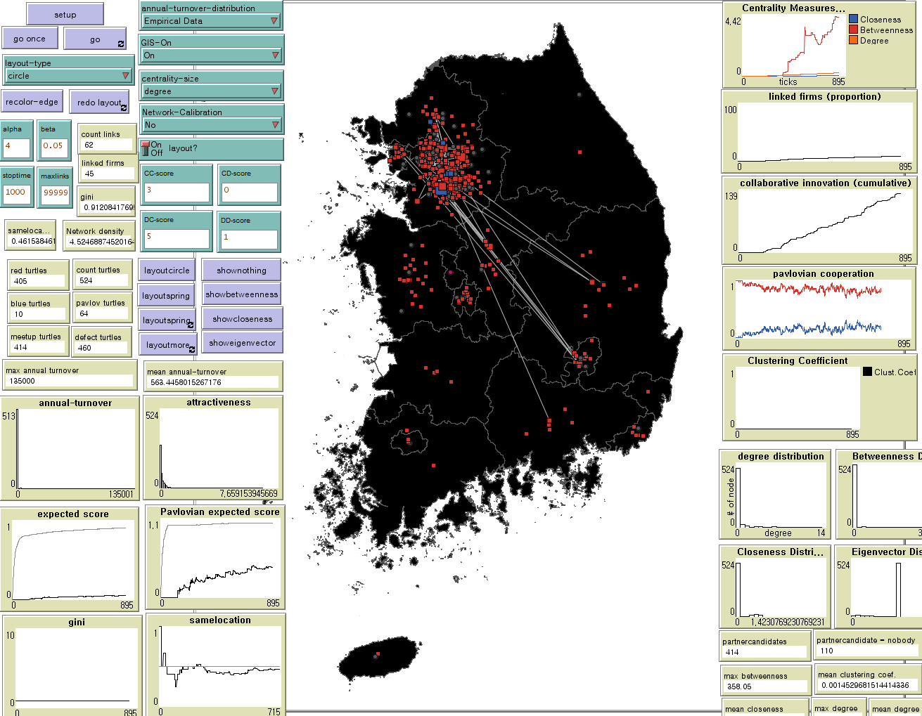
Since the coefficients for validation were composed of 10 \(\alpha\) and 6 \(\beta\), the total number of possible combinations was 60. Each combination was simulated 30 times until the average number of edges was 70 (see Appendix)[5]. Therefore, the simulation was performed 1,800 times in total. The screenshot of the simulation run on Netlogo is shown in Figure 2.
This study explored the combination of parameters with the lowest mean absolute percentage error (MAPE) between the simulation results and the observations for the above seven indicators. The equation for the MAPE is as follows:
| $$ \textit{MAPE}=\frac{100}{n}\sum_{i=1}^n \left|\frac{Y_i-S_i}{Y_i} \right|$$ |
\(Y_i\) represented the observed value, \(S_i\) indicated the simulated value and n referred to the number of observations used as indicators. Lower MAPE values indicate higher forecasting performance because the values generated in the model are simillar to the empirical data. Figure 3 presents the MAPE for the 60 combinations used in the validation in order from the lowest to highest value.
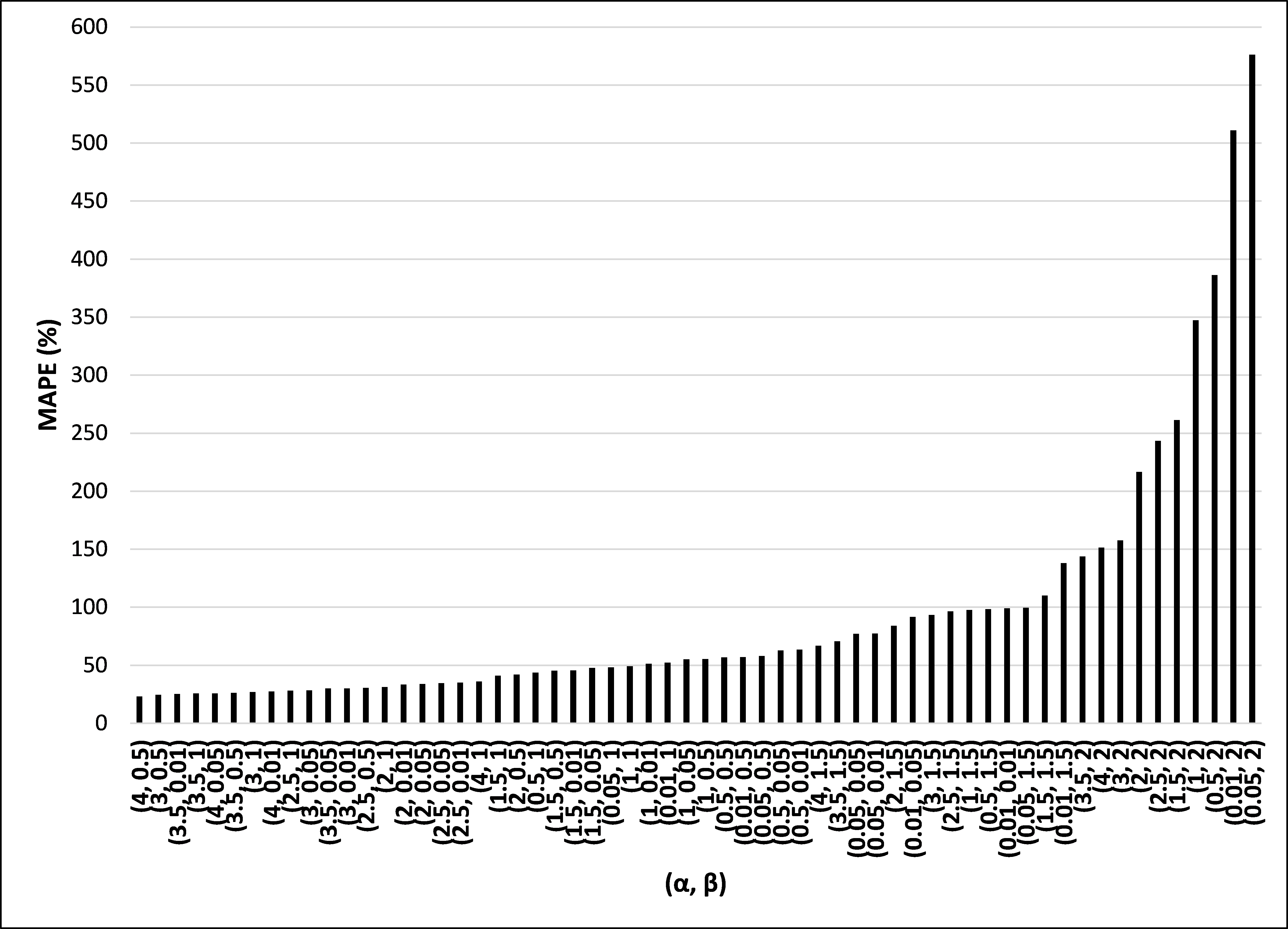
This study adopted \(\alpha\) = 4 and \(\beta\) = 0.5, which was the smallest combination of the MAPE (23.27%). The validation results indicate that inter-firm collaborative innovation is associated more with firm size factors, such as sales, than by geographic distance. In other words, even if the distance between the firms is not large, it does not associate with collaborative innovation. However, if the firms' sales are high, the probability of collaborative innovation increases exponentially. Table 3 presents the comparison between the mean of the simulation results and the empirical data.
| Network Characteristics | Empirical Data | Simulated Data (30 Iterations) | ||
| Mean | SD | 95% CI | ||
| Edges | 70 | 70.167 | 8.263 | (67.081, 73.252) |
| Linked Firms | 64 | 49.933 | 3.248 | (48.721, 51.146) |
| Max. Degree | 18 | 12.767 | 1.942 | (12.042, 13.492) |
| Mean Degree | 0.267 | 0.268 | 0.032 | (0.256, 0.280) |
| Mean Betweenness Centrality | 7.101 | 4.876 | 0.933 | (4.527, 5.224) |
| Mean Closeness Centrality | 0.048 | 0.033 | 0.005 | (0.031, 0.035) |
| Mean Clustering Coefficient | 0.008 | 0.008 | 0.004 | (0.006, 0.009) |
| MAPE | 23.27% | |||
Experiments of FSD and Its Effect on Collaborative Innovation
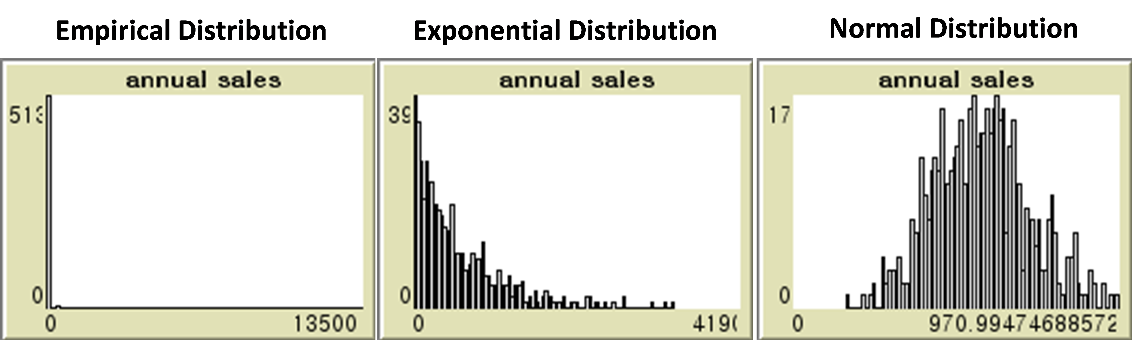
I experimented with the effect of firm size distribution on collaborative innovation, using (1) empirical distribution, (2) exponential distribution, and (3) normal distribution as independent variables. The mean values of these distributions were the same, but there was a difference in the polarization level of the annual sales between firms.
The empirical distribution was extremely polarized, which was similar to the exponential distribution but had a more skewed distribution. Most firms were located in the lowermost section of the tenth quartile, and the Gini coefficient was 0.9121, indicating the high level of size heterogeneity. The exponential distribution is a random exponential distribution with a mean equal to the empirical distribution but a smaller variance. The Gini coefficient was 0.5024, and the level of size heterogeneity was medium. The normal distribution is the random normal distribution with the mean being equal to the empirical distribution and the standard deviation being 25% of the mean. The Gini coefficient was 0.1409, and the level of size heterogeneity as low. Table 4 summarizes the characteristics of these distribution scenarios.
| Firm Size Distribution (Annual Sales Distribution) | |||
| Empirical | Exponential | Normal | |
| Description | Empirical distribution | Random exponential distribution | Random normal distribution |
| Mean 563.45 Max 13,500 | Mean 563.45 | Mean 563.45 SD: 25% of the mean | |
| Gini Index | 0.9121 | 0.5024 | 0.1409 |
| Firm Size Heterogeneity | High | Medium | Low |
Figure 4 presents the histogram for each distribution.
Collaborative innovation occurs when Pavlovian agents cooperate mutually. The simulations were performed up to 936 ticks with an average edge count of 70 in the empirical distribution, and 30 iterations were performed for each distribution. In an undirected network, the network density (\(D\)) was calculated using nodes (\(N\)) and the actual connections (\(A\)). Also, cooperative behaviour (CB) was calculated using the number of Pavlovian agents at time \(t (PA_t)\) and Pavlovian agents performing cooperative actions at time \(t (POC_t)\). Table 5 shows the manipulation settings for the simulation.
| Type | Variable | Description | Measurement |
| Dependent Variable | Collaborative Innovation | Frequency of Collaborative Innovation | Sum of Collaborative Innovation in the Industry |
| Independent Variable | Level of Firm Size Heterogeneity | FSD (Annual Sales Distribution) | Empirical Distribution (High Heterogeneity) |
| Exponential Distribution (Medium Heterogeneity) | |||
| Normal Distribution (Low Heterogeneity) | |||
| Control Variable | Payoff | Payoff (R, T, S, P) | \(R\) = 3, \(T\) = 5, \(S\) = 0, \(P\) = 1 |
| Partnering Mechanism | Huff Parameter | \(\alpha\) = 4, \(\beta\) = 0.5 |
Figure 5 presents screenshots of the simulation over time.
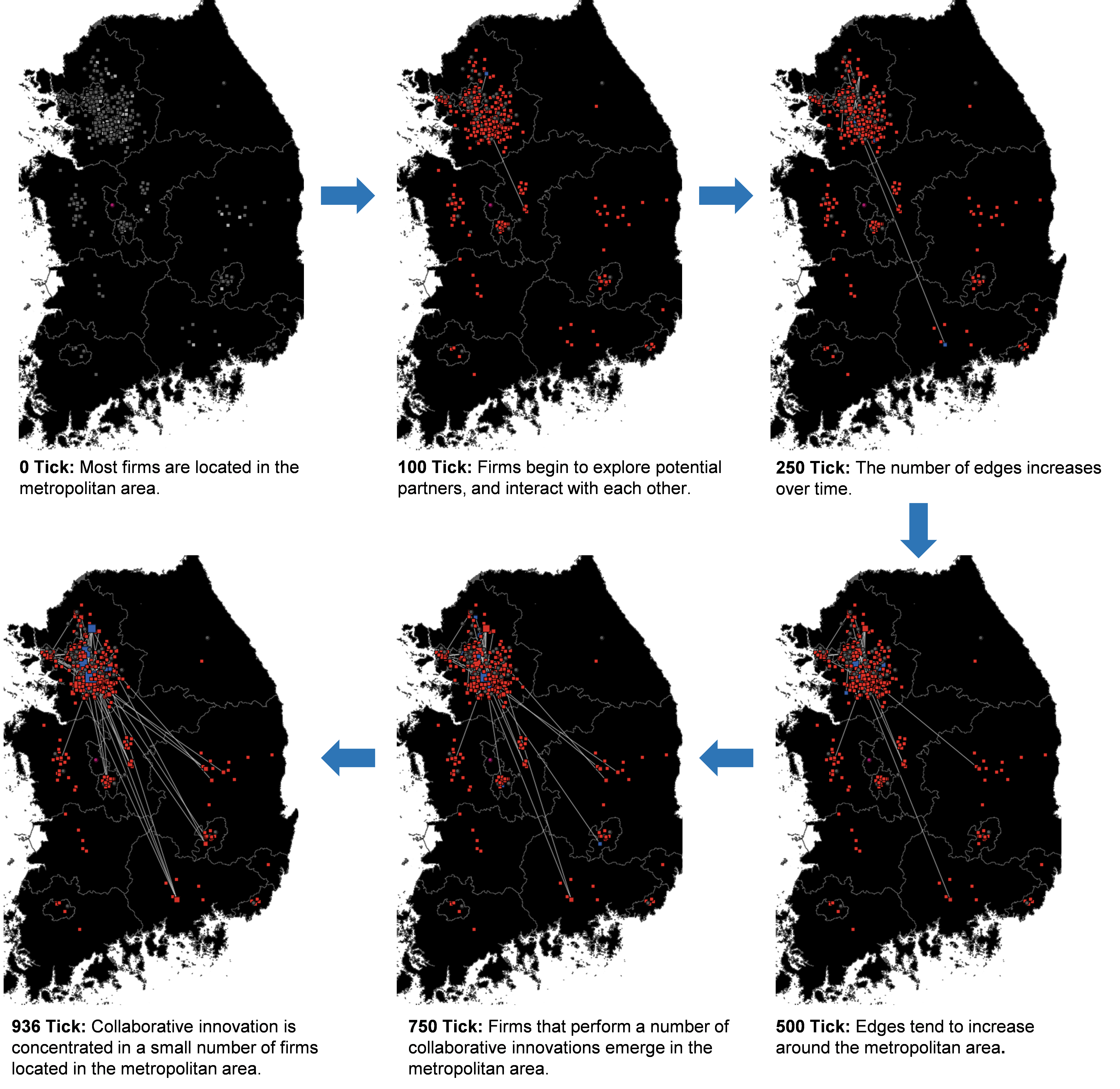
At the beginning of the simulation, the network was not formed but, as time passes, the edges were created due to cooperation between the firms. The red agents represent firms that have defected, and the blue agents represent firms that have cooperated — the size of the agent increases in proportion to its degree. At the endpoint of 936 ticks, a small number of firms were found to be relatively larger than the other firms, indicating that the unequal distribution of degrees observed in the real world was successfully reproduced through this agent-based model.
Experimental Results
Results
In this experiment, I investigated changes in collaborative innovation according to changes in FSD. The simulation investigated whether there was a difference between the firms' collaborative innovation by the level of size heterogeneity using the ANOVA for the sum of the frequencies of collaborative innovation performed by all firms until tick = 936. Figure 6 presents the ANOVA results for collaborative innovation by FSD.
| Variable | Source | SS | df | MS | F | Prob.>F |
| Collaborative Innovation | Between Groups | 591261.42 | 2 | 295630.71 | ||
| Within Groups | 60551.73 | 87 | 696.00 | 424.76\(\ast\ast\ast\) | 0.0000 | |
| Total | 651813.16 | 89 | 7323.74 |
The results show that the effect of firm size heterogeneity on collaborative innovation is statistically significant at the 99.9% significance level. The effects are presented in Figure 6.
Collaborative innovation increased by about 1.5 times in the exponential distribution and 2.3 times more in the normal distribution than in the empirical distribution, indicating that it is sensitive to the level of firm size heterogeneity. Figure 6 shows that as firm size heterogeneity decreases, the frequency of collaborative innovation increases. This finding suggests that collaborative innovation is performed more frequently when the FSD in the industry is relatively uniform than when the size heterogeneity is large. Therefore, as the firm size heterogeneity decreases, the tendency to engage in collaborative innovation among firms is relatively high. In conclusion, the results of this analysis suggest that, as the firm size heterogeneity decreases, the frequency of collaborative innovation in the industry becomes higher.
Sensitivity analysis
Sensitivity of behaviour
I also performed a sensitivity analysis to check the robustness of the model. One of the most popular sensitivity analysis methodologies to assess robustness in ABM is the one-factor-at-a-time (OFAT) method (Broeke, Voorn, & Ligtenberg 2016). The OFAT method is a method of analysing the relationship between one independent variable and a dependent variable according to the change of the independent variable. Broeke et al. (2016) called the OFAT method an important methodology for revealing the relationship between valid parameters and outputs.
I performed OFAT sensitivity analysis for \(\alpha\) and \(\beta\), respectively. In all scenarios, 30 iterations were performed. Figure 7 shows the results of OFAT sensitivity analysis for \(\alpha\).
The changes in collaborative innovation show a similar pattern until \(\alpha\) decreases from 4 to 2. When \(\alpha\) is less than 0.5, there is no significant observable change in collaborative innovation, according to FSD. This finding implies that the effect of firm size distribution on collaborative innovation is not significant when the weight for firm size is 1 or less. It is sensible that firm size distribution does not have a significant effect on collaborative innovation if firms consider firms’ size less critical. Conversely, a similar pattern is observed when weighing the firm size by more than 1, suggesting that this model is robust against \(\alpha\). Therefore, the sensitivity analysis results showed that the model is robust against \(\alpha\), as long as it weights the size when the firm seeks a collaboration partner. Next, Figure 8 shows the results of the OFAT sensitivity analysis for \(\beta\).
The changes in collaborative innovation show a similar pattern until \(\beta\) increases ten times from 0.05 to 0.5. When \(\beta\) is 1 or more, the pattern of change of collaborative innovation, according to FSD, reverses. When \(\beta\) is increased by about 60 times to 3, collaborative innovation decreases with firm size heterogeneity. The results show that, in an industry in which geographical distance is critical for partner selection, the patterns of change of collaborative innovation according to firm size heterogeneity may differ. It is, therefore, not surprising that the effect of firm size distribution decreases as companies weigh the distance between the firm size and the distance in selecting partners. Therefore, the sensitivity analysis results show that this model is robust against \(\beta\) as long as it does not weigh two times more geographical distance than the base model when selecting a collaboration partner. The result implies that the policy to reduce the constraint of geographical distance between firms, such as the R&D cluster, can be an effective way to activate collaborative innovation, even in the case of firm size heterogeneity.
Sensitivity of strategy
Fifteen percent of innovative firms in the study have participated in collaborative innovation as Pavlovian firms and the rest as defective firms. This is a strong assumption that may affect the results. Therefore, I performed the OFAT sensitivity analysis on the proportion of Pavlovian firms. In all scenarios, 30 iterations were performed. Figure 9 shows the results of the OFAT sensitivity analysis according to the proportion of Pavlovian firms.
Changes in collaborative innovation show almost the same pattern for all conditions, except for the "0% scenario". No collaborative innovations are performed under the condition that the proportion of Pavlovian firms is 0%, and as the percentage of Pavlovian firms increased, the total frequency of collaboration innovations increased. This pattern indicates that the model works properly. Collaboration innovation increases as the heterogeneity in the FSD decreases under all conditions until the proportion of Pavlovian firms increases from 15% to 100%. The sensitivity analysis shows that the model is robust against firm strategy.
Discussion and Conclusions
This study developed an agent-based model to analyse the effect of firm size heterogeneity on collaborative innovation in the industry. The model was developed based on an NIPD game and was validated using collaborative innovation data of Korean ICT firms. The base model developed in this study successfully replicated the collaborative innovation patterns of Korean ICT firms.
The simulation results indicate that a decrease in the firm size heterogeneity appears to have a positive effect on collaborative innovation in the industry. This result implies that an increase in the firm size heterogeneity can reduce firms' collaborative innovation and further impede the open innovation ecosystem in the industry. Sensitivity analysis results showed that the model is robust as firms consider size as an important factor when selecting partners.
This study contributes to the theoretical development of innovation research and confirms that firm size heterogeneity is an essential variable for collaborative innovation in industries. The FSD has previously been suggested by some researchers to be an important independent variable that affects performance within an industry (Malerba 2005), but it has failed to advance further from the theoretical discussion due to practical limitations. This study attempts to mitigate the methodological constraints by using the agent-based model and report that firm size heterogeneity has significantly associated with collaborative innovation. Thus, it is necessary to shift the focus of the discussion beyond the current research trend, which focuses only on the firm, to the industry level.
This study also contributes to the government policy to create an open innovation ecosystem in an industry. Collaborative innovation is not actively performed in an industry with size heterogeneity is attributable not only to the payoffs (Chiang 1995; Majeski 1986) but also to size heterogeneity itself. The results show that collaborative innovation in the industry is sensitive to firm size heterogeneity. Therefore, governments need to mitigate the firm size heterogeneity to create an open innovation ecosystem in an industry. For example, governments can strengthen the protection of software intellectual property rights of SMEs to prevent unfair practices such as large firms' software imitation and technology theft. Also, the government can expand SME-eligible industries and items in the field of ICT, such as software through public procurement. In sum, it is possible to expand not only the regulation of large firms’ unfair practices but also the improvement of the structure of large firms’ labour force and the opportunities for SMEs entering the market through public procurement (Kim 2012).
Finally, the model built in this study can be used for policy experiments. Chiang (1995) showed that it is possible to experiment with policy options that promote collaboration by adjusting T and R in PD games. Subsequent studies should explore the impact of policy alternatives using this model.
Model Limitations
The model was built to explore the effects of the skewness of the FSD on collaborative innovation; however, it does not consider the reverse causality. Firms can grow in the long run by participating in collaborative R&D projects to enhance their innovation capacity (Belderboss, Carree & Lokshin 2004). However, the model assumes that the FSD is fixed over time. Since this model does not consider the reverse causality, the interpretation from the causal point of view is limited. Additionally, this model does not include firms’ selection process driven by market mechanisms. The payoffs by firms' behaviours are fixed, making changes in size distribution independent of market outcomes such as revenue. This assumption can hinder the model's expandability, and the size distribution can have a significant impact on endogenous innovation factors (Cabral & Mata 2003; Panago & Schivardi 2003). Thus, it is reasonable to assume that changes in the size distribution affect the payoffs of the model, which may affect firms’ partner selection. Subsequent studies should aim to improve the model by replicating the success and failure process of firms with the changes in endogenous innovation factors caused by the changes in size distribution.
Finally, this study replicated the collaborative innovation network through parameter calibration using the Huff model to simplify the model. However, preferential attachment rules based on various proximities can influence partner selection (Capone & Lazzeretti 2018). Subsequent studies should aim to develop an extended model that can analyse various collaborative characteristics, such as the persistence of collaborative innovation, by including these proximity factors.
Acknowledgements
I would like to thank Dr. Jeong Hun Park, Dr. Sukwon Lee, Dr. Taehyon Choi, Dr. Eungab Kim, and Dr. Il Hwan Chung for their helpful comments. I also appreciate valuable comments and suggestions from Dr. Yushim Kim. Finally, I thank the editor, Dr. Flaminio Squazzoni, and anonymous reviewers for their constructive comments and support.Model Documentation
The model has been built in Netlogo (Wilensky 1999). The source code of the model is available at https://www.comses.net/codebases/2e083d1e-9224-4af5-802f-3d6f53c7bbc3/releases/1.1.0/.Notes
- DART: https://dart.fss.or.kr/.
- NDSL: http://www.ndsl.kr.
- The GIS data were collected from Geoservice (http://www.gisdeveloper.co.kr).
- The basic module of the NIPD game follows Wilensky (2002).
- The maximum tick was 1,000
Appendix
The following figures show the simulation results of each indicator according to the combination of \(\alpha\) and \(\beta\). Each figure represents the values when the mean of the number of edges is 70, which is the same as the observed value at 30 iterations. The figures enable us to capture changes in network characteristics by each parameter. Changes in edges by \(\alpha\) and \(\beta\) are shown in Figure 10.
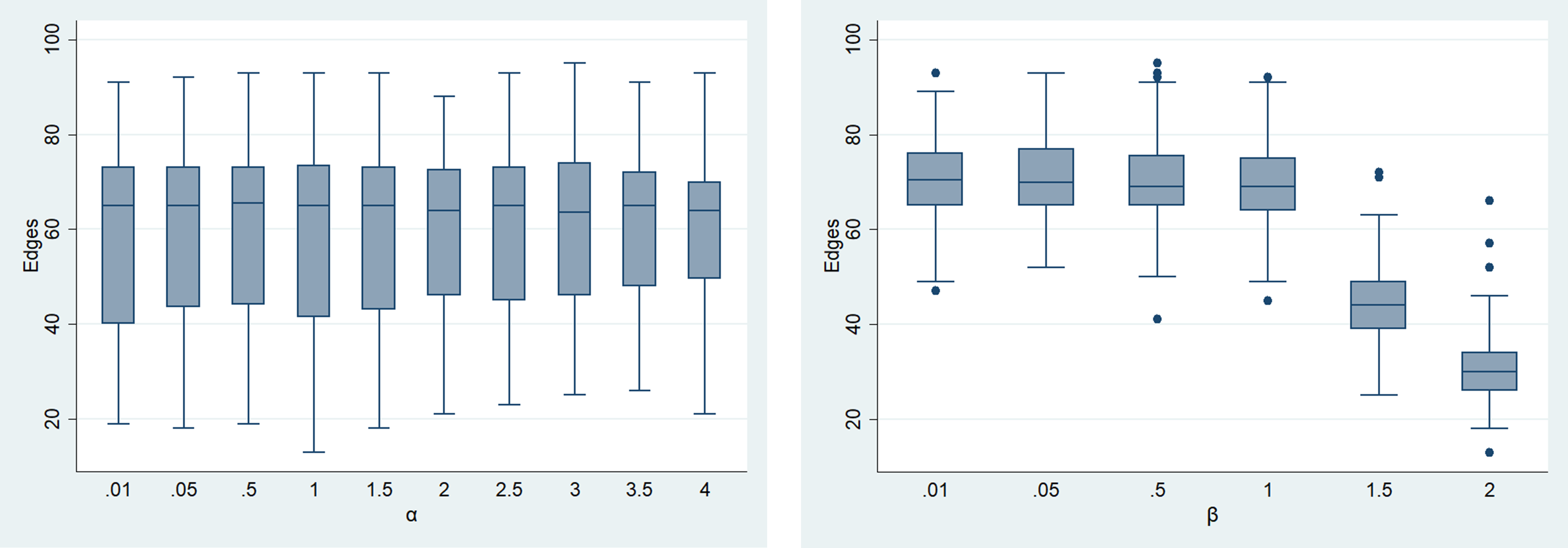
A significant change in the edge by \(\alpha\) is not observed. However, when \(\beta\) is 1 or higher, edges are generated at 70 or less at the maximum tick, and, as \(\beta\) increases, the number of generated edges also decreases gradually. Changes in linked firms are presented in Figure 11.
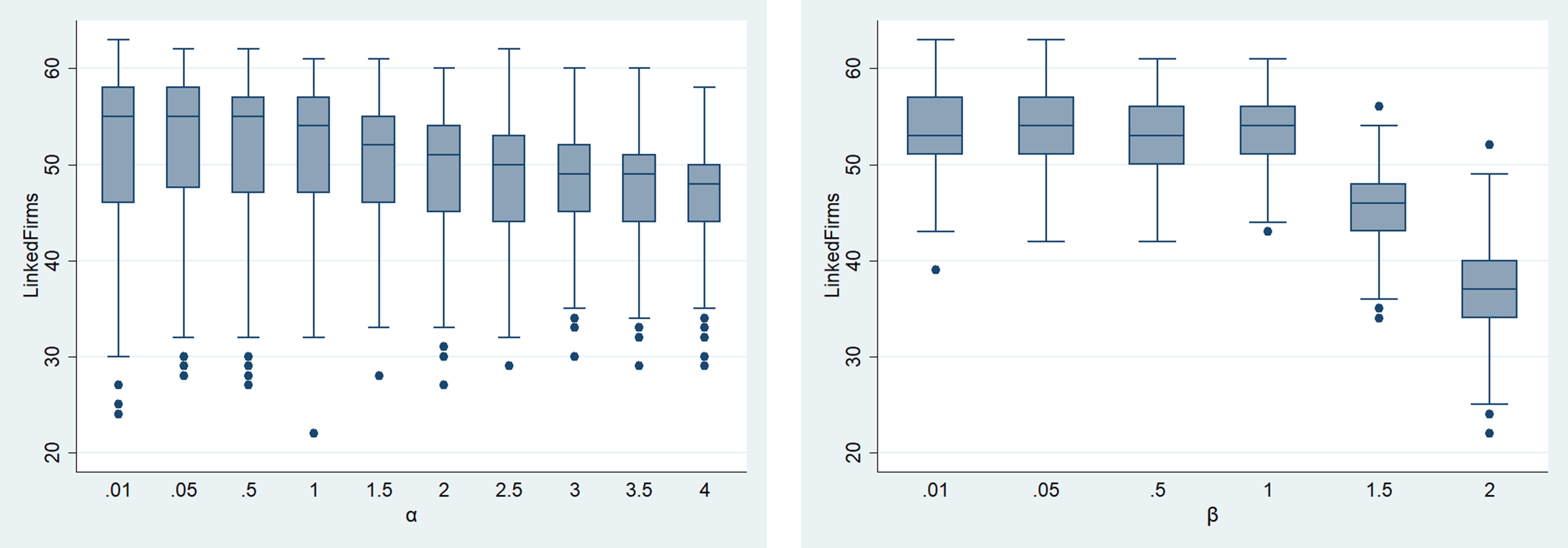
The number of linked firms tends to decrease slightly with an increasing \(\alpha\). The number of firms linked to \(\beta\) tends to decrease rapidly from 1 and decreases to less than 40 when \(\beta\) is 2. The number of edges and linked firms is more affected by \(\beta\) than by \(\alpha\). Changes in maximum degree and mean degree are shown in Figure 12.
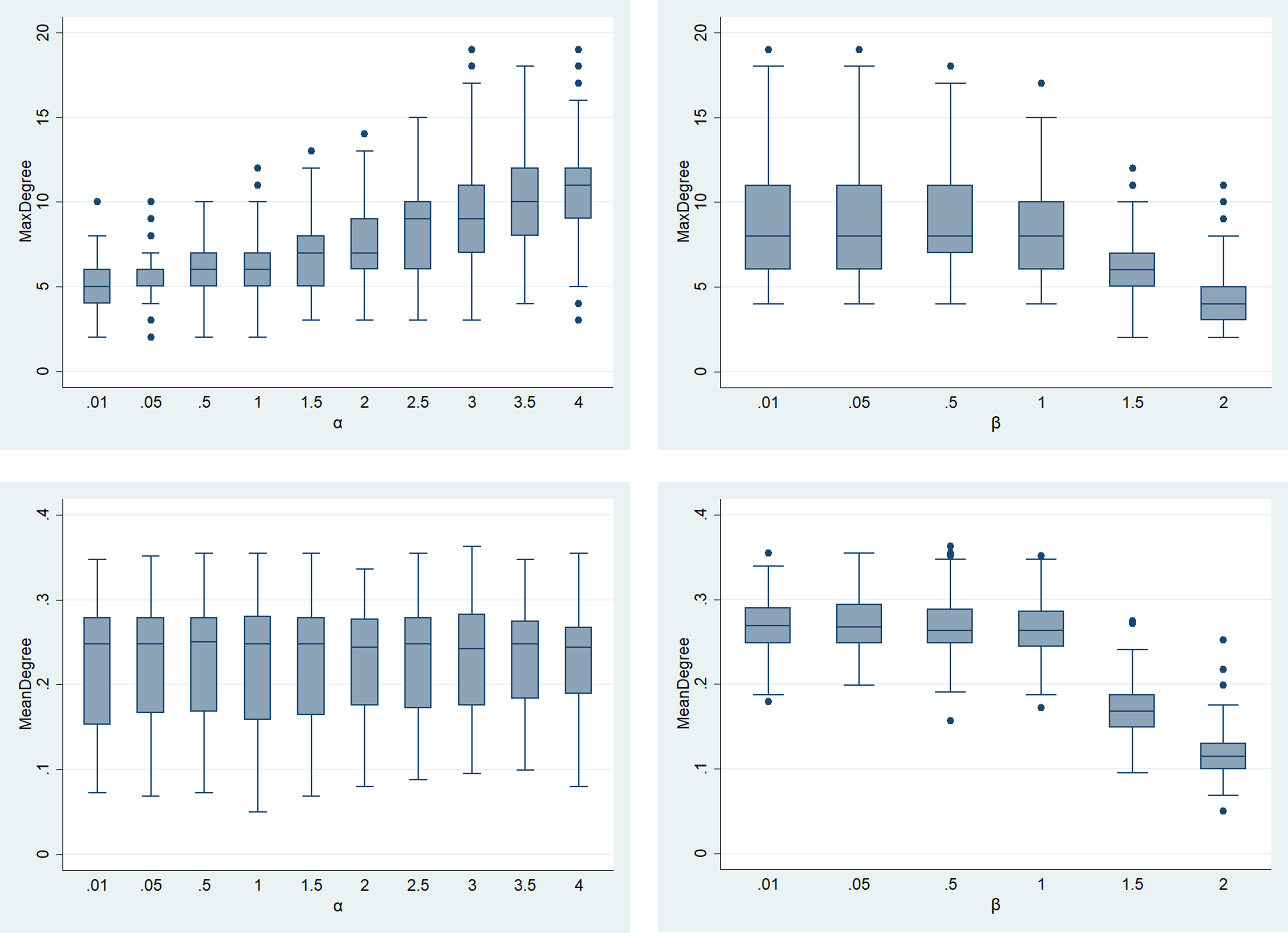
The maximum degree tends to increase as \(\alpha\) increases but decreases as \(\beta\) increases. The mean degree is more sensitive to \(\beta\) than it is to \(\alpha\) and decreases rapidly when \(\beta\) is greater than 1. Changes in mean betweenness centrality and mean closeness centrality are shown in Figure 13.
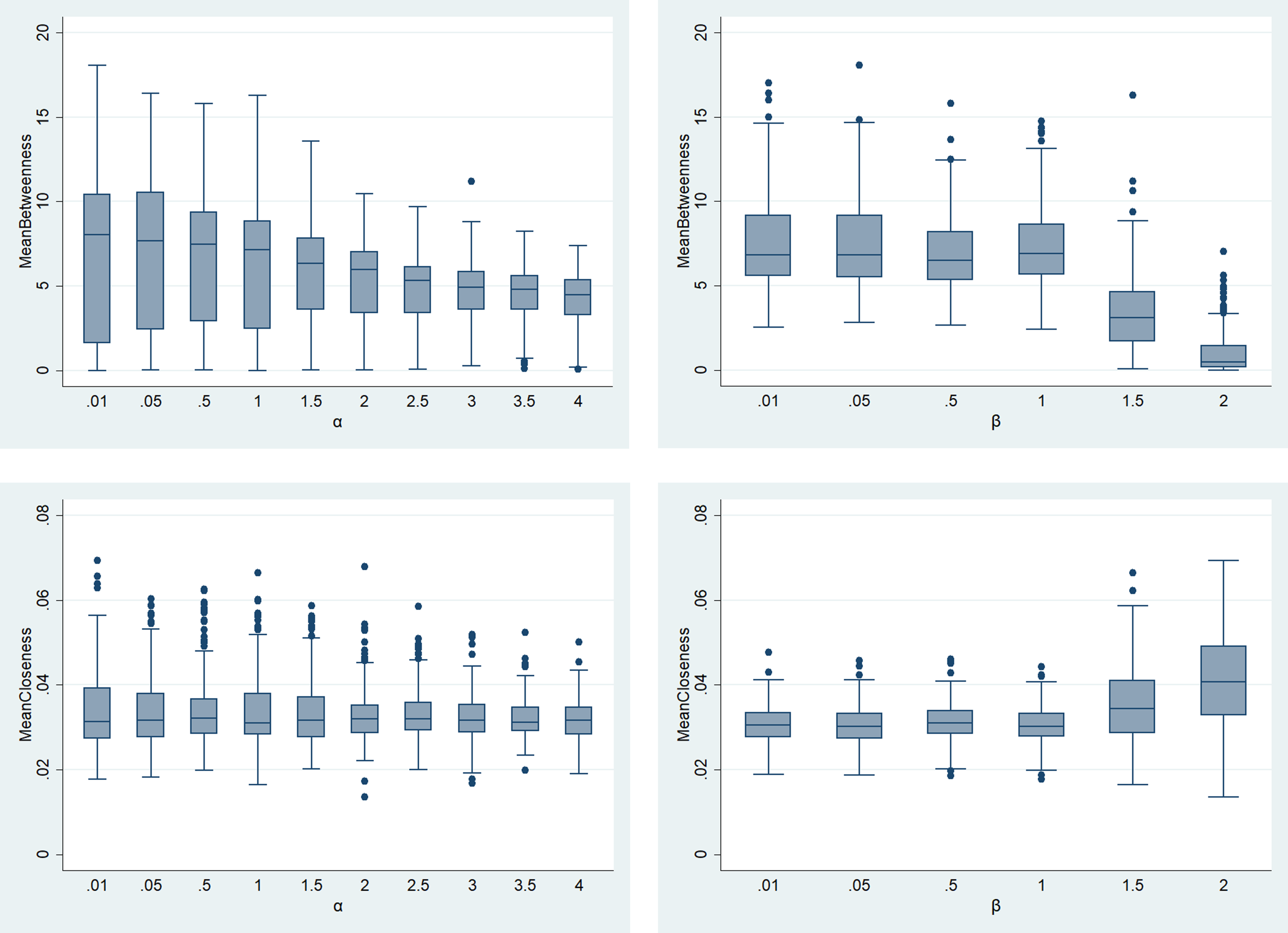
The mean betweenness centrality decreases as the value of \(\alpha\) increases and decreases significantly when \(\beta\) is greater than 1. The mean closeness centrality does not change with \(\alpha\), but it increases when \(\beta\) is 1 or higher. Changes in the mean clustering coefficient are shown in Figure 14.
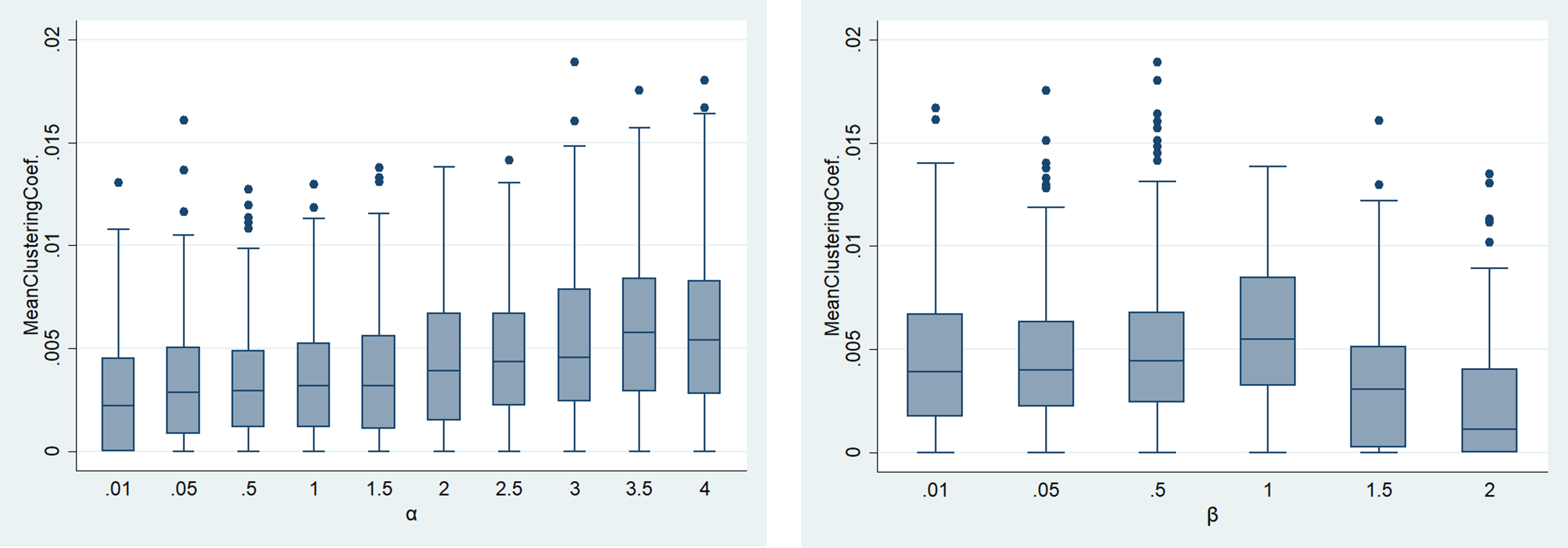
The mean clustering coefficient tends to increase slightly as \(\alpha\) increases and decreases sharply when \(\beta\) exceeds 1. This study performs parameter calibration based on the results, and the forecasting accuracy of the 60 combinations for the seven network indicators is presented in Figure 3.
References
ANGELINI, P., Cerulli, G., Cecconi, F., Miceli, A., & Potì, B. (2017). R&D Subsidization Effect and Network Centralization: Evidence from an Agent-Based Micro-Policy Simulation. Journal of Artificial Societies and Social Simulation, 20(4), 4. https://www.jasss.org/20/4/4.html. [doi:10.18564/jasss.3494]
AREND, R. J. (2009). Reputation for Cooperation: Contingent Benefits in Alliance Activity. Strategic Management Journal, 30(4), 371-385. [doi:10.1002/smj.740]
AREND, R. J., & Seale, D. A. (2005). Modeling alliance activity: An iterated prisoners' dilemma with exit option. Strategic Management Journal, 26(11), 1057–1074. [doi:10.1002/smj.491]
ARRIGHETTI, A., Landini, F., & Lasagni, A. (2014). Intangible assets and firm heterogeneity: Evidence from Italy. Research Policy, 43(1), 202-213. [doi:10.1016/j.respol.2013.07.015]
ARSENYAN, J., Büyüközkan, G., & Feyzioğlu, O. (2015). Modeling collaborative formation with a game theory approach. Expert Systems with Applications, 42(4), 2073-2085. [doi:10.1016/j.eswa.2014.10.010]
AXELROD, R. (1984). Evolution of Cooperation. New York: Basic Books.
AXELROD, R. (1997). The Complexity of Cooperation: Agent-Based Models of Competition and Collaboration. Princeton, NJ: Princeton University Press.
AXTELL, R. L. (2001). Zipf distribution of U.S. firm sizes. Science, 293(5536), 1818-1820. [doi:10.1126/science.1062081]
BABUTSIDZE, Z. (2016). Innovation, competition, and firm size distribution on fragmented markets. Journal of Evolutionary Economics, 26(1), 143-169. [doi:10.1007/s00191-015-0425-5]
BELDERBOSS, R., Carree, M., & Lokshin, B. (2004). Cooperative R&D and firm performance. Research Policy, 33(10), 1477-1492. [doi:10.1016/j.respol.2004.07.003]
BRENNER, T. (2004). Agent Learning Representation - Advice in Modelling Economic Learning. Papers on Economics and Evolution. Jena: Max Planck Institute.
BROEKE, G. T., Voorn, G. V., & Ligtenberg, A. (2016). Which sensitivity analysis method should I use for my agent-based model? Journal of Artificial Societies and Social Simulation, 19(1), 5, https://www.jasss.org/19/1/5.html
BUTTS, C. T., Acton, R. M., & Marcum, C. S. (2012). Interorganizational collaboration in the Hurricane Katrina response. Journal of Social Structure, 13, 1-36.
CABRAL, L., & Mata, J. (2003). On the evolution of the firm size distribution: Facts and theory. American Economic Review, 93(4), 1075-1090. [doi:10.1257/000282803769206205]
CANTNER, U., & Hanusch, H. (2001). Heterogeneity and evolutionary change: Empirical conception, findings, and unresolved issues. In J. Foster and J. S. Metcalfe (eds.), Frontiers of Evolutionary Economics. Competition, Self-Organization, and Innovation Policy. Cheltenham, UK, Northampton, Massachusetts, USA: Edward Elgar. [doi:10.4337/9781843762911.00020]
CAPONE, F., & Lazzeretti, L. (2018). The different roles of proximity in multiple informal network relationships: Evidence from the cluster of high technology applied to cultural goods in Tuscany. Industry and Innovation 25(9), 897–917. [doi:10.1080/13662716.2018.1442713]
CATULLO, E. 2013. An agent-based model of monopolistic competition in international trade with emerging firm heterogeneity. Journal of Artificial Societies and Social Simulation, 16(2), 7, https://www.jasss.org/16/2/7.html. [doi:10.18564/jasss.2155]
CEAUSU, I. & Bourbonnais, R. (2014). IT SMEs in France and Romania. FAIMA Business & Management Journal, 2(3), 49-60.
CERULLI, G. (2012). Are R&D subsidies provided optimally? Evidence from a simulated agency-firm stochastic dynamic game. Journal of Artificial Societies and Social Simulation, 15(1), 7. https://www.jasss.org/15/1/7.html [doi:10.18564/jasss.1886]
CHIANG, J. T. (1995). Application of game theory in government strategies for industrial collaborative research and development. Technology in Society, 17(2), 197-214. [doi:10.1016/0160-791x(95)00003-a]
CHO, Y., Yang, I., Suh, Y., & Jeon, J. (2015). Analysis of Current Situation and Relationship among National R&D Projects for Technology Convergence. Journal of the Korean Institute of Industrial Engineers, 42(3), 305-323. [doi:10.7232/jkiie.2015.41.3.305]
D’ESTE, P. (2005). How do firms’ knowledge bases affect intra-industry heterogeneity? An analysis of the Spanish pharmaceutical industry. Research Policy, 34 (2005), 33-45. [doi:10.1016/j.respol.2004.10.007]
FREEMAN, C. (1979). Centrality in social networks conceptual clarification. Social Networks, 1(2), 215-239. [doi:10.1016/0378-8733(78)90021-7]
GIBRAT, R. (1931). Les inegalites economiques, applications: aux inegalites des richesses, a la concentration des entreprises, aux populations des ville, aux statistiques des familles, etc., d’une loi nouvelle, la loi de l’effet proportionnel. Paris: Librarie du Recueil Sirey.
GULATI, R., Khanna, T. & Nohria, N. (1994). Unilateral commitments and the importance of process in alliances. Sloan Management Review, 35(3), 61–69.
HENREKSON, M., & Johansson, D. (1999). Institutional effects on the evolution of the size distribution of firms. Small Business Economics, 12(1), 11–23.
HESHIMATI, A., & Lenz-Cesar, F. (2015). Policy simulation of firms’ cooperation in innovation. Research Evaluation, 24 (2015), 293-311.
HUFF, D. L. (1964). Defining and estimating a trading area. Journal of Marketing, 28(3), 34-38. [doi:10.1177/002224296402800307]
ITU. (2016). Measuring the information society report 2016, Geneva: ITU Report.
JOHANSSON, D. (2004). Is small beautiful? The case of the Swedish IT industry. Entrepreneurship & Regional Development, 15, 271-287. [doi:10.1080/0898562042000263258]
JUNG, J. H., & Hong, J. P. (2015). A study on the network structure of the supplier-customer relations between flagship and small companies. The Korean Small Business Review, 37(4), 77-103.
KELLY, M., Schaan, J. L., & Joncas, H. (2002). Managing alliance relationships: Key challenges in the early stages of collaboration. R&D Management, 32, 11-37. [doi:10.1111/1467-9310.00235]
KIM, J. H. (2012). Interpretation of polarization between large firms and SMEs. Seoul: KDI Report.
KISDI. (2007). 2007 Korea IT industry outlook. Seoul: Korea Information Society Development Institute.
KOGUT, B. (1988). Joint ventures: Theoretical and empirical perspectives. Strategic Management Journal, 9(4), 319– 332. [doi:10.1002/smj.4250090403]
LEE, K. (2009). An analysis of the polarization of profitability between large corporations and small- and medium-sized enterprises (SMEs) and economic growth. Seoul: KIF Report.
LEIPONEN, A. (2002). Why do firms not collaborate? Competencies, R&D collaboration, and innovation under different technological regimes. In A. Kleinknecht and P. Monhen (Eds.), Innovation and Firm Performance: Econometric Explorations of Survey Data. London: Palgrave. [doi:10.1057/9780230595880_11]
MAGGIONI, M., & Uberti, E. (2007). Inter-regional knowledge flows in Europe: An econometric analysis. In K. Frenken (Ed.), Applied Evolutionary Economics and Economic Geography. Cheltenham: Edward Elgar. [doi:10.4337/9781847205391.00023]
MAJESKI, S. J. (1986). Technological innovation and cooperation in arms races. International Studies Quarterly, 30, 175-191. [doi:10.2307/2600675]
MALERBA, F. (2005). Sectoral systems of innovation: A framework for linking innovation to the knowledge base, structure, and dynamics of sectors. Economics of Innovation and New Technology, 14(1-2), 63-82. [doi:10.1080/1043859042000228688]
MARTIN, S. (2002). Spillovers, appropriability, and R&D. Journal of Economics, 75(1), 1-32.
MCMILLAN, G. S., Mauri, A. L. & Casey, D. L. (2014). The scientific openness decision model: “Gaming” the technological and scientific outcomes. Technological Forecasting and Social Change, 86, 132-142. [doi:10.1016/j.techfore.2013.08.021]
MONTOBBIO, F., & Sterzi, V. (2013). The globalization of technology in emerging markets: A gravity model on the determinants of international patent collaborations. World Development, 44(C), 281-299. [doi:10.1016/j.worlddev.2012.11.017]
MORESCALCHI, A., Pammolli, F., Penner, O., Peterson, A. M., & Riccaboni, M. (2015). The evolution of networks of innovators within and across borders: Evidence from patent data. Research Policy, 44(3), 651-668. [doi:10.1016/j.respol.2014.10.015]
NA, J., Lee, J. D., & Baek, C. (2017). Is the service sector different in size heterogeneity? Journal of Economic Interaction and Coordination, 12(1), 95-120. [doi:10.1007/s11403-015-0152-x]
NELSON, R. R., & Winter, S. G. (1982). An Evolutionary Theory of Economic Change. Cambridge, MA.: Belknap Press of Harvard University Press.
NODA, T., & Collis, D. J. (2001). The evolution of intra-industry firm heterogeneity: Insights from a process study. Academy of Management Journal, 44(4), 897-925. [doi:10.2307/3069421]
NORDMANN, A. (2004). Converging Technologies - Shaping the Future of European Societies. Brussels: European Commission.
NOWAK, M., & Sigmund, K. (1993). A strategy of win-shift, lose-stay that outperforms tit-for-tat in the prisoners' dilemma game. Nature, 364, 56-58. [doi:10.1038/364056a0]
ÖZMAN, M. (2008). Network formation and strategic firm behaviour to explore and exploit. Journal of Artificial Societies and Social Simulation, 11(1), 7. https://www.jasss.org/11/1/7.html.
PANAGO, P., & Schivardi, F. (2003). Firm size distribution and growth. Scandinavian Journal of Economics, 105(2), 255-274.
PARK, S. H., & Ungson, G. R. (1997). The effect of national culture, organizational complementarity, and economic motivation on joint venture dissolution. Academy of Management Journal, 40(2), 279-307. [doi:10.2307/256884]
PICCI, L. (2010). The internationalization of inventive activity: A gravity model using patent data. Research Policy, 39(8), 1070-1081. [doi:10.1016/j.respol.2010.05.007]
POWER, C. (2009). A spatial agent-based model of n-person prisoner's dilemma cooperation in a socio-geographic community. Journal of Artificial Societies and Social Simulation, 12(1), 8. https://www.jasss.org/12/1/8.html
RICHIARDI, M. (2004). Generalizing Gibrat: Reasonable multiplicative models of firm dynamics. Journal of Artificial Societies and Social Simulation, 7(1), 2, https://www.jasss.org/7/1/2.html.
ROCO, M. 2007. National Nanotechnology Initiative-Past, Present, Future. In: Goddard, W. et al. (Eds.) Handbook on Nanoscience, Engineering and Technology, 2nd Edition. Oxford: Taylor and Francis. [doi:10.1201/9781420007848.ch3]
SCHERNGELL, T., & Barber, M. (2009). Spatial interaction modelling of cross-region R&D collaborations: Empirical evidence from the 5th EU framework programme. Regional Science, 88(3), 531-546. [doi:10.1111/j.1435-5957.2008.00215.x]
SCHWEITZER, F., Behera, L., & Muhlenbein, H. (2002). Evolution of cooperation in a spatial prisoner's dilemma. Advances in Complex Systems, 5(2&3), 269-299. [doi:10.1142/s0219525902000584]
SQUAZZONI, F., & Boero, R. (2002), Economic performance, inter-firm relations, and local institutional engineering in a computational prototype of industrial districts. Journal of Artificial Societies and Social Simulation, 5(1). https://www.jasss.org/5/1/1.html.
STEERS, R. M., Shin, Y., & Ungson, G. R. (1989). The Chaebol: Korea’s New Industrial Might. New York, NY: Harper & Row.
SUZUMURA, K. (1992). Cooperative and noncooperative R&D in an oligopoly with spillovers. The American Economic Review, 82(5), 1307-1320.
SZILAGYI, M. N., & Szilagyi, Z. C. (2002). Non-trivial solutions to the n-person prisoner's dilemma. Systems Research and Behavioral Science, 19(3), 281-290. [doi:10.1002/sres.435]
TESFATSION, L. (2006). ‘Agent-based computational economics: A constructive approach to economic theory’. In K. Judd and L. Tesfatsion (Eds.), Handbook of Computational Economics, vol. 2: Agent-Based Computational Economics. Amsterdam: North-Holland. [doi:10.1016/s1574-0021(05)02016-2]
WALTMAN, L. (2011). Computational and game-theoretic approaches for modeling bounded rationality (Doctoral dissertation). Retrieved from http://www.ludowaltman.nl/.
WATTS, C., & Gilbert, N. (2014) Simulating Innovation: Computer-Based Tools for Rethinking Innovation. Cheltenham: Edward Elgar Publishing.
WILENSKY, U. (1999). NetLogo. Center for connected learning and computer-based modeling. Northwestern University. Retrieved from http://ccl.northwestern.edu/netlogo/.
WILENSKY, U. (2002). NetLogo PD N-Person iterated model. Center for Connected Learning and Computer-Based Modeling, Northwestern University. Retrieved from http://ccl.northwestern.edu/netlogo/models/PDN-PersonIterated.
WILLIAMSON, O. E. (1981). The Economics of Organization: The Transaction Cost Approach. American Journal of Sociology, 87(3), 548-577. [doi:10.1086/227496]
WINDRUM, P., Fagiolo, G., & Moneta, A. (2007). Empirical validation of agent-based models: Alternatives and prospect. Journal of Artificial Societies and Social Simulation, 10(2), 8. https://www.jasss.org/10/2/8.html.
YAMAMOTO, H., Ishida, K., & Ohta, T. (2004). Modeling reputation management system on online C2C market. Computational & Mathematical Organization Theory, 10(2), 165-178. [doi:10.1023/b:cmot.0000039169.05361.3d]
YANG, H-L., & Wu, T. C. T. (2008). Knowledge sharing in an organization. Technological Forecasting and Social Change, 75(2008), 1128-1156. [doi:10.1016/j.techfore.2007.11.008]
YUN, J. J., Won, D., & Park, K. (2016). Dynamics from open innovation to evolutionary change. Journal of Open Innovation: Technology, Market, and Complexity, 2(7), 1-22. [doi:10.1186/s40852-016-0033-0]
YURTSEVEN, A. E., & Tandoğan, V. S. (2012). Patterns of innovation and intra-industry heterogeneity in Turkey. International Review of Applied Economics, 26(5), 657-671. [doi:10.1080/02692171.2011.631900]