
Introduction
Many grand challenges—global warming, loss and fragmentation of forest areas, biodiversity loss, wildlife extinction, desertification, and the like—are besetting humanity at unprecedented rates. Yet virtually all these grand challenges can be traced back to rapidly growing human population and various human activities. Humans are degrading or destroying ecosystems at an alarming rate, jeopardizing their vital “life-support services of tremendous value” such as food, water, clean air, soil, and forests (Daily & Matson 2008; Assessment 2005). Even so-called protected areas are not exempted from such degradation worldwide (c et al. 2004; Liu et al. 2001). Facing such crisis, the International Convention of Biological Diversity’s Aichi targets (https://www.cbd.int/sp/target/) have called for protecting natural habitats (Target 5), threatened species (Target 12), and various ecosystem services from natural ecosystems (Target 14). The United Nations’ 17 Sustainable Development Goals, especially Goal 15, also aim to protect, restore, and promote sustainable use of terrestrial ecosystems (United Nations 2016).
Payments for ecosystem services and challenges
In response to the above challenges, payments for ecosystem services (PES) have been employed for decades, aiming to provide incentives directly to resource users to take actions or to refrain from previous actions to protect ecosystems and many services of tremendous value to humanity. As a result, a growing body of PES literature has focused on the mechanism and efficacy of PES programs, exploring what factors—be they socioeconomic, demographic, and environmental conditions — may help sustain beneficial changes in PES participants’ behavior (Friess, Phelps, Garmendia, & Gómez-Baggethun 2015; Wunder 2005).
Despite many reported successes in restoring ecosystems and improving human wellbeing, a set of challenges have surfaced in many PES programs. First, PES programs lack sustainability because many participants return to their pre-PES behavior once PES payment ends. This problem has been observed not only in developing countries such as China (Uchida, Xu, & Rozelle 2005) but also in developed countries such as USA (Claassen, Cattaneo, & Johansson 2008). Existing PES research has focused on individual factors including agricultural income, land productivity, distance from household to land parcel, land plot slope, age of contract holders, labor supply, and livelihood alternatives (Adhikari & Agrawal 2013; Engel 2016; He & Sikor 2015). These variables, though very important, are treated in a piecemeal manner, overlooking complex features (e.g., feedback loops, nonlinear relationships) among them. Second, there is a dire need to measure the ecological performance of PES programs by more than just land use and land cover (LULC). Very few PES programs and program evaluations have considered faunal and/or detailed floral responses due to PES programs (for exceptions see Liu et al. 2008; Tuanmu et al. 2016), which are equally important as LULC measures (Scullion, Thomas, Vogt, Pérez-Maqueo, & Logsdon 2011). Therefore, Lewison, An, & Chen (2017) suggest that PES research and implementation consider “the complex interrelationship among socioeconomic, demography and ecological metrics” while developing and testing more representative ecological metrics.
China’s Grain-To-Green Program (GTGP) provides an excellent opportunity to address these challenges. In response to the massive flooding in 1998, the Chinese central government started GTGP around 1999 (Phase I) and renewed it in 2007 (Phase II), aiming to reduce soil erosion and protect its natural environment through tree planting (“Green”) in steep farmland areas (>15⁰ in northwestern China and 25⁰ in southwestern China; Liu, Li, Ouyang, Tam, & Chen 2008). Farmers are compensated through cash, rice, or corn (“Grain”) to maintain or increase their economic well-being (Liu & Diamond 2005; Liu et al. 2008). The 3rd phase of GTGP started in 2017 with increased payment level and total amount of enrollment (State Forestry Administration of China 2017).
Complex systems
Research on complex systems aims to understand complex systems, which often include heterogeneous subsystems or elements, autonomous entities, nonlinear relationships and thresholds, legacy effects and time lags, resilience, and multiple interactions and feedback loops among them (Axelrod & Cohen 1999; Levin et al. 2013; Liu et al. 2007). Such systems often feature path-dependence, self-organization, difficulty of prediction, and emergence not analytically tractable from system components and their attributes alone—particularly surprising outcomes observable as a result of human-nature couplings (Council 2014). These generic features have been found in six empirical complex systems studies (Liu et al. 2007), as well as in many other sites (Irwin & Geoghegan 2001; Malanson, Zeng, & Walsh 2006; Messina & Walsh 2005).
The increasing popularity of agent-based modeling (ABM)[1] in modeling and understanding complex human-environment systems is rooted in challenges we face: Most major challenges in such systems involve autonomous, decision-making agents such as people and animals. The high level of complexity in these systems makes it extremely difficult, if not impossible, to represent and simulate these systems in a controlled way. ABM, based on the object-oriented programming (OOP) paradigm, represents the related entities and subsystems as agents at various, often hierarchical, levels. Employing flexible rules to mimic relevant actions of agents and many complex relationships and interactions, ABM satisfies the needs of understanding complex systems (An, Linderman, Qi, Shortridge & Liu 2005; An et al. 2014). Hence it is suggested that an ABM approach be employed to understand, harness, and improve (rather than fully control) the system’s structure and function, taking innovative actions to steer the system in beneficial directions (Axelrod & Cohen 1999).
Goal and research questions
The complex systems approach offers a great potential to understand the cascading impacts of many ecological / environmental, socioeconomic, and demographic factors in a spatially and temporally explicit manner when their complex, reciprocal relationships are considered. The goal of this paper is therefore to measure and project the social-ecological impacts of PES over a relatively long term. We will use not only land use and land cover metrics as in previous studies, but also wildlife occupancy indicators.
Specifically, we aim to answer three questions: 1) what are the effects of PES on human demography, livelihoods, and related activities? 2) what are the spatially explicit effects of PES on wildlife habitat use after incorporating human demography, livelihoods, and related activity data? Moreover, 3) what factors may make PES programs ineffective in the long run?
Methods
Study site
Fanjingshan National Nature Reserve (FNNR), located in the northeast part of Guizhou Province, China, is a flagship reserve of subtropical ecosystems in China (Figure 1). FNNR is part of the 25 global biodiversity hotspots (Myers, Mittermeier, Mittermeier, da Fonseca, & Kent 2000), replete with over 6000 plant, animal, and bird species (GDF & FNNR 1990). Totaling 419 km2 in area[2], the reserve (roughly 27.5°N – 28.0°N and 108.55°E - 108.8°E) encompasses low elevation (700 m) evergreen broadleaf ecosystems, mixed deciduous-broadleaf ecosystems at mid-elevations (1000-1300 m), and subalpine, meadow, and conifer ecosystems at higher elevations (1600-2600 m), manifesting large variability in biophysical conditions (Yang, Lei, & Yang 2002). The reserve is also home of the last and only population (around 750 animals) of the Guizhou golden monkeys (Rhinopithecus brelichi; GGMs hereafter), also known as Guizhou snub-nosed monkeys, an umbrella, engendered species highly sensitive to human presence, activity, and the resultant habitat degradation (Yang, Lei, & Yang 2002).

FNNR is home of over 13,000 villagers (70% are Tujia and Miao minorities), who live within or near FNNR boundaries in a subsistence lifestyle. These villagers are allowed to enter non-core habitat areas for resource collection and livestock herding, though illegal production of charcoal, wood collection, and poaching in the core habitat area also occur occasionally year round (Yost et al. 2020). Over the last two decades, local villagers have increasingly migrated to cities for higher-pay jobs, and only returned to the home villages for short times (e.g., during a spring festival). Migration in this paper is defined as outmigration outside of county boundaries, and the dominating migration destinations are coastal big cities. The total number of out-migrants was 350 (57.85%) out of all the 605 households we surveyed in 2014 (Sections 2.4-2.5). In 2001 when GTGP started, there were very few out-migrants (10 for all 350 migrants). Once GTGP was in operation, a substantial (near exponential) increase in the number of migrants occurred, suggesting that the related laborers, once released due to GTGP, may have migrated out at a slower pace at earlier times yet at an accelerated speed later. We therefore consider GTGP to be a trigger and catalyst of migration because it not only freed labor that had been bonded to farmland, but also provided a start-up fund (e.g., for travel expenses) for those relatively poor households to migrate out.
This study focuses on the northern area of FNNR, where two villages (Taohuayuan and Pingsuo) closest to Yangaoping (approximately 29.97°N, 108.75°E) are located. Yangaoping is the breeding area where GGMs gather to mate in April and September (the red circle in Panel D, Figure 1). Human settlements typically are located around the borders of the reserve, which are at lower elevations.
Social survey
We administered household interviews in 2014. Using the roster of all 3,256 households used in the 2013 FNNR census as our sampling frame, we surveyed 605 households (yellow squares in Panel A, Figure 1) based on a stratified random sampling strategy (detail in Yost et al. 2020). The survey focused on 1) individual-level characteristics: age, gender, education level, etc. of each member in the surveyed household; 2) household characteristics: living conditions, household economy including incomes, expenses, and time, number of people, and income related to migration and local off-farm jobs; 3) household land use and PES characteristics: total land area, amount of time (labor), and income or compensation related to GTGP; and 4) household extraction of local resources: time, frequency, amount, and location (recorded in Google Earth maps) related to various resources (Yost et al. 2020).
In 2015, we revisited all these 605 households with similar questions, although focus was more on household land use, participation in GTGP, and detailed household income. We ended up with a survey of 494 households in 2015. In 2016 we surveyed all households in five natural villages within two administrative villages of Pingsuo and Taohuayuan (blue triangles in Panel A, Figure 1). The aim was to obtain full coverage of all households in these two administrative villages for agent-based modeling, verification, and data analysis purposes. We surveyed all the available households in these two administrative villages, ending up with a total of 94 households. All the surveys were conducted under permits from the San Diego State University’s Institutional Review Board (Protocol #: 1732093).
Ecological survey
To investigate vegetation structure and habitat use of wildlife under human disturbance, we established 71 sampling plots in FNNR. Each plot was 20 m x 20 m (a subset of them is shown as pentagons in Panel D, Figure 1). Location of plots was decided based on accessibility, elevation, distance to other plots, and suggestions provided by FNNR staff and local field guides with the goal to spread out plots across FNNR. For each plot, we recorded species of understory, midstory, and overstory vegetation and estimated the percentage of cover for each species. We also deployed a Bushnell Trophy Cam infrared camera at each plot to monitor presence of mammals (>0.5 kg) and pheasants from April 2015 to January 2018, relocating cameras to other places to increase site diversity (Chen et al. 2020). Typically, cameras were mounted on trees 0.3 to 1 m above the ground. We set cameras at auto-sensitivity to record three photos upon each detection, with a 1-second delay between photographs. Field efforts were conducted under permits from the San Diego State University’s Institutional Animal Care and Use Committee (Protocol #: 14-01-002L). The camera-trap photos, after downloaded from the cameras, were processed via Adobe Bridge, a photo-formatting and tagging program. Due to our focus on the Guizhou golden monkeys (GGMs hereafter), data processing focused on the 44 presence points (Mak 2019). The data were then imported into Excel to process the point data in a csv file.
Agent-based modeling
We constructed an agent-based model (ABM) that integrates environment and ecology, human demographics and livelihoods, PES policy, and their interactions. The agent-based model aims to simulate the 94 households for which we have collected detailed demographic, livelihood, and activity data, while some rules in the ABM are based on the 605 and 494 households surveyed in 2014 and 2015, respectively (Section Social survey). We choose a 5-day temporal resolution, which is a compromise of the following considerations. First, some processes need finer resolutions—for instance, local people’s resource collection takes place daily. Second, other processes are recorded or operate at coarser resolutions, and examples include local people’s migration and returning farmland to forestland or fallow (data recorded at monthly or yearly levels). Lastly, choosing a coarser temporal resolution makes simulation much faster. We choose to simulate over 20 years (1460 time-steps) using the ABM, a time span that is long enough to allow for observable changes in the FNNR complex human-environment system but not too long to bring in much uncertainty in simulation outcomes.
Environment and ecology
The ABM creates an 85 x 100 grid spanning the entire FNNR, with a spatial resolution of approximately 300 m. The spatial resolution is chosen to balance the need to represent seasonal movement of monkey family-groups and human resource extraction activities and simulation speed. Among the 8500 cells within the lattice, 4897 are within the FNNR boundary with the following attributes assigned to them: elevation and 13 land cover or use types: Bamboo, Coniferous, Broadleaf, Mixed Forest, Lichen, Deciduous, Shrublands, Clouds, Farmland, Household, Farm, PES Forest, and Outside_FNNR. These vegetation categories were generated through a combination of supervised and unsupervised image classification routines from near-anniversary-date summer Landsat 5 satellite imagery (Tsai et al. 2016). Elevation data were extracted from a 30 m ASTER DEM GeoTIFF released by NASA in 2011 (Tsai et al. 2016).
Our representation of the environment and ecology is from two aspects. First, we incorporate land use and land cover data as mentioned above. Second, we use golden monkey habitat occupancy as an indicator of intactness of a certain land area for GGM habitat use (the inverse of this measure is the degree of human intrusion):
| $$\text{Occupancy} = \text{# of simulated GGM visits on a pixel per year}$$ | (1) |
Our choice of this occupancy measure is based on the ecology of GGMs: They avoid direct encounter with humans (Yang et al. 2002). This metric for the impact of PES programs enables us to address the need to quantify broader, ecological dimensions of PES as mentioned in Section PES and Challenges.
Guizhou golden monkeys (GGMs)
With GGM life traits well-documented (e.g., Bleisch et al. 1993; Wu et al. 2004; Yang et al. 2002; Zhang et al. 2016) an agent-based model was developed and posted online, which simulates the 750 GGM agents’ seasonal movement and their life events such as birth, death, and grouping (Mak 2019). The literature shows that GGMs live and travel in family groups of 20-45, while larger groups (Bleisch et al. 1993; Yang et al. 2002) and all-male groups[3] are observable. Yet in the model larger groups of more than 45 individuals were split into two. For space limit we do not elaborate other GGM features in the model (Mak 2019).
Building on Mak (2019), the ABM in this paper models GGM habitat use or occupancy primarily with consideration of elevation, vegetation types, and avoidance of human presence in the context of human livelihoods and demographic changes. This modeling choice also hinges upon the fact that FNNR has high primary forest cover, representing excellent habitat that provides food and water for golden monkeys (detail in Yang et al. 2002, p. 43). This situation makes it reasonable to not incorporate GGM feeding or water seeking behavior in our model.
GGMs prefer to stay in areas from 1500[4] to 1700 m (Wu et al. 2004), and in extreme situations to 2300 m (Bleisch et al. 2008). Accordingly, the model limits GGM family-groups to elevations between 1000 m and 2200 m, human settlements (i.e., they escape when approaching a radius = 400[5] m centering each settlement), farms (radius = 300 m), and GTGP enrolled land parcels (radius = 200 m). Finally, whenever away from human settlements, GGM family-group agents either move according to free semi-random walk based on their vegetative surroundings or are traveling to and from Yangaoping in mating and breeding seasons. The monkey agents tend to stay in mixed, deciduous, conifer-broadleaf, and broadleaf forests, but also travel through other types of vegetation (Bleisch et al. 1993; Wu et al. 2004; Yang et al. 2002; Zhang et al. 2016).
Human demographics and livelihoods
The ABM generates land parcel objects (one special kind of agents) that belong to a total of 94 household agents. Then the model assigns household attributes (e.g., household ID, village, x and y coordinates, dryland area, paddy land area, GTGP land area, non-GTGP land area) to each of these parcels. These parcels may convert between GTGP and non-GTGP land uses, depending on the PES program implemented within the model as well as a set of socio-demographic variables (Section GTGP participation and land use). A sum of 370 human agents are also created with individual attributes such as person ID, age, gender, education level, marriage status, and working status (work on own farm, off-farm agricultural work, non-farm business, being student, not working, unable to work) assigned to each agent based on the survey data. Each person agent goes through relevant life events: being born, growth, going to college, marriage (simultaneously bringing in a female or male from outside the two villages[6]), bearing a child, death, migration (outmigration and re-migration listed below separately), and collecting resources. For space limit, we give detail of bearing children (for the rest we refer interesting readers to the Python code at https://www.comses.net/codebases/0852f2b8-6517-4b83-b7fa-8304eb538421/releases/1.0.0/):
Once a woman reaches 20 (the minimum age for a woman to marry), assign her a birth plan (or fertility rate) representing the number of children for her whole life: she may have 0, 1, 2, 3, 4, or 5 children in her whole life with the probabilities of 0.03125, 0.15625, 0.3125, 0.3125, 0.15625, and 0.03125 (An et al. 2005). The average birth plan is 2.5 children per woman.
When 1~3 years (a parameter that is randomly chosen to be 1, 2, or 3 years) elapse since her marriage (i.e., she reaches 20 years old), she may have her 1st child. Then after another 1~3 years (another parameter that is randomly chosen to be 1, 2, or 3 years), she may have her 2nd child…till her birth plan is accomplished (An et al. 2005).
Resource extraction
Based on our survey data of the 94 households, each household sends a person agent to designated cells to collect resources such as fuelwood, medicinal herbs, bamboo shoots, mushroom, fodders (for pigs and oxen), and others while the order of collecting these resources is randomly chosen. At each time step, the person agent only gathers one resource at a time. The person agent is usually the household head (if within the range of 15-59 years old); if s/he migrates out, the next capable person is designated as a substitute head of household and collect these resources.
When human agents venture out to collect resources at a certain time step, their paths are marked to act as a barrier at the same step for GGM family-group agents that travel around the reserve freely but avoid humans. Along with human avoidance and seasonal migration to breeding habitat (the circle in Panel A, Figure 1), Guizhou snub-nosed monkeys also avoid low elevations and choose weighted semi-random paths based on favored vegetation.
Each person agent gathers this resource at the corresponding frequency determined by the 2016 survey. Each time a resource collection action takes often one day, part of the 5-day time step that includes the day. During the step, all the cells that the person agent traverses (from the household cell to the collection cell) receive a weight of 1/5 for avoidance. This weight is proportional to the collection frequency. The mismatch in temporal resolution may affect the influence human presence exerts on GGM habitat use, which will be discussed in Section Discussion. Human resource gathering and other activities in the northern area (Panel A, Figure 1) may be suppressed with influences such as higher income or higher rates of human out-migration. Below we describe how we represent outmigration.
Outmigration
Modeling human decision has been a big challenge in understanding and envisioning human-environment systems, and ABM may offer unique power in this regard (An 2012). Migration happens only if the household under consideration has a person between 15 and 59. According to our field survey in 2015 (Yang 2019), the annual probability of outmigration can be calculated based on a logistic function:
| $$\textit{mig_prob} = \Bigl( \textit{eLogit} / (\textit{exp_Logit} + 1) / 45 \Bigr)$$ | (2) |
| $$\begin{split} \textit{eLogit} &= \exp(2.07 - 0.00015\,*\,\textit{income_local_off_farm} + 0.67 \,* \,\textit{num_labor} + 4.36 \,*\, \\ & \textit{migration_network} - 0.58\, *\, \textit{non_gtgp_land_per_labor} + 0.27 \,*\, \textit{gtgp_part} - 0.13 \,* \\ & \textit{age} + 0.07 \,*\, \textit{gender} + 0.17\, *\, \textit{education }+ 0.88 \,*\, \textit{marriage }+ 1.39 \,*\, \textit{farm_work }+ 0.001 \\ & *\,\textit{mig_remittances}) \end{split}$$ | (3) |
However, the migrants can choose to return to their rural home, and we model the corresponding probability as a function of the age at the time of the most recent migration (age) and the number of years s/he has migrated out (yr_mig) according to a logistic regression by Yang (2019):
| $$\textit{re_mig_prob} = \exp(-1.2+0.06 \ast \textit{age}-0.08 \ast \textit{yr_mig})/(-1.2+0.06\ast \textit{age} - 0.08\ast \textit{yr_mig}) $$ | (4) |
Therefore, a person might migrate out, return, re-migrate out, and continue this cycle if s/he is between 15 and 59 years old and the randomly generated numbers are less than the probabilities determined by Equations 2 and 4 are greater than the threshold. The coefficients in Equations (3) and (4) are results of the above-mentioned logistic regression based on survey data collected in 2015 (Yang 2019).
GTGP participation and land use
The ABM reads in parcel level data for each household from a CSV file. The CSV file contains whether a parcel is enrolled in GTGP (named a GTGP parcel) or not (named a non-GTGP parcel), x and y coordinates, whether the land is dryland or paddy land (land_type), and the amount of time to travel to the corresponding land parcel from the household (time_land).
Local farmers may fallow some parcels even without any payment for various reasons. Therefore we combine fallowing of land with GTGP participation, resulting in an action of returning farmland to other uses, including planting cash crops, fallowing land, or planting ecological trees (Yost et al. 2020). A logistic function is used to calculate the probability of returning farmland to other uses (including participating in GTGP and leaving the parcel fallow) at parcel level. Yet for terminology consistency and conciseness, we still call it GTGP participation and the corresponding probability is named GTGP_par_prob :
| $$\begin{split} \textit{GTGP_par_prob} &= \exp(2.52 - 0.012 \ast \textit{Age} - 0.29 \ast \textit{Gender} + 0.01 \ast \textit{Education} + 0.001 \ast \textit{hh_size} \\ & - 2.45\ast \textit{land_type} + 0.0006 \ast \textit{GTGP_net_cash} + 0.04 \ast \textit{time_land}) / \\ & (1 + \exp (2.52 - 0.012 \ast \textit{Age} - 0.29\ast \textit{Gender}+ 0.01\ast \textit{Education} + 0.001\ast \textit{hh_size} \\ & - 2.45\ast \textit{land_type}+ 0.0006\ast \textit{GTGP_net_cash}+ 0.04\ast \textit{time_land})) \end{split}$$ | (5) |
This equation was derived through logistic regression analysis based on data from 2015 (Yang 2019), where land_type and time_landare explained earlier, and GTGP_net_cash is the difference between GTGP payment and income from growing crops on the same land parcel.
When enrolling non-GTGP parcels, there are three conditions to meet simultaneously. First, the area of non-GTGP land in the household must be greater than or equal to 0.3 \(mu\) (a parameter based on the data from 2015; subject to sensitivity analysis) to provide vegetables. Second, a randomly generated number is less than the probability calculated using Equation 5. Third, the GTGP payment is greater than zero. Note that if GTGP payment is zero (GTGP ends), there is still a small chance that the household may fallow the parcel (as mentioned earlier we still call this action participating in GTGP for terminology conciseness) at a much lower probability. This low probability defaults at GTGP_par_prob * 0.25, where parameter 0.25 is based on data from 2015 and subject to sensitivity analysis (same for 0.3 below).
When deciding to reconvert a GTGP parcel to non-GTGP parcel (i.e., farmland), a very small probability (GTGP_par_prob* 0.25) is calculated, where 0.25 is a parameter subject to sensitivity analysis (Section Model evaluation). Once a parcel is enrolled in GTGP, it will be reconverted to farmland once a randomly generated number is less than this small probability.
Model evaluation
The model evaluation is comprised of two elements: model verification that warrants that the code does what it intends to do and is free of coding bugs, and model validation that compares model structure, processes, and results with expected ones based on data, theory, or experts’ opinions (An et al. 2005; Manson 2002). As model verification is progressive (debugging continues), the results below contribute to both verification and validation.
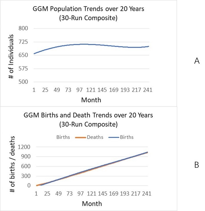
We first show the dynamics of model projected human population size, births, deaths, and number of migrants[7] over 20 years (on a monthly basis) (73x20 steps) for the two villages in the northern area (Figure 2). As we do not have empirical data for population size after 2016, we are not able to compare our projected population sizes with empirical data. Instead, we calculate various measures such as population increase rate, births, and deaths, and then compare them with data from other sources. The overall population dynamics shows a slow increase (i.e., from 370 in 2016 to around 400 in 2036), which can be explained by the accumulated numbers of births, deaths, and migrants in Table 1: There are 85 births and 54 deaths, implying natural increase of 31 persons. There are 27 marriages, bringing in 27 people from outside. So the total number of increase in population size is 31 + 27 = 58; if subtracting the increase in number of out-migrants (105-76=29), the total increase through migration is 58-29 = 29 persons. So the total population in 2036 should be 370 (base) + 29 = 399, which explains the simulated population size 399.40 in Year 2026 (or Step 1458) in Table 1. These results exactly corroborate the projected population size in Month 240 (Year 20) in Figure 2 (under BP = 2.5). When birth plan (fertility rate) is set to be 1.5 and 3.5, the total population in 2036 changes to 366 and 435, respectively (see more in Section Experiment design and Experiment results).
We also validate these demographic results using external data and information. From the simulation results in Table 1, the annual birth rate is (72-0)/(20x 370) = 0.973%, or 9.73‰. According to China’s National Bureau of Statistics (2018), the nationwide birth rate is 1.093% or 10.94‰. Considering the decreasing trend in the most recent 20 years (e.g., from 14.03‰ in 2000 to 10.94‰ in 2018), our average annual rate of 9.73‰ for the next 20 years is reasonable. Similarly we calculate the annual death rate to be (54-0)/(20x 370)=0.730% or 7.30‰, while the same national rate is 7.09% in 2016 (National Bureau of Statistics 2017).
| Step | Population | Births | Deaths | Marriages | Laborers | Migrated |
| 6 | 370.80 | 0 | 0.17 | 0 | 160.6 | 76.20 |
| 732 | 391.87 | 47.30 | 25.03 | 14.73 | 122.70 | 93.37 |
| 1458 | 399.40 | 84.80 | 53.73 | 27.33 | 106.33 | 105.40 |
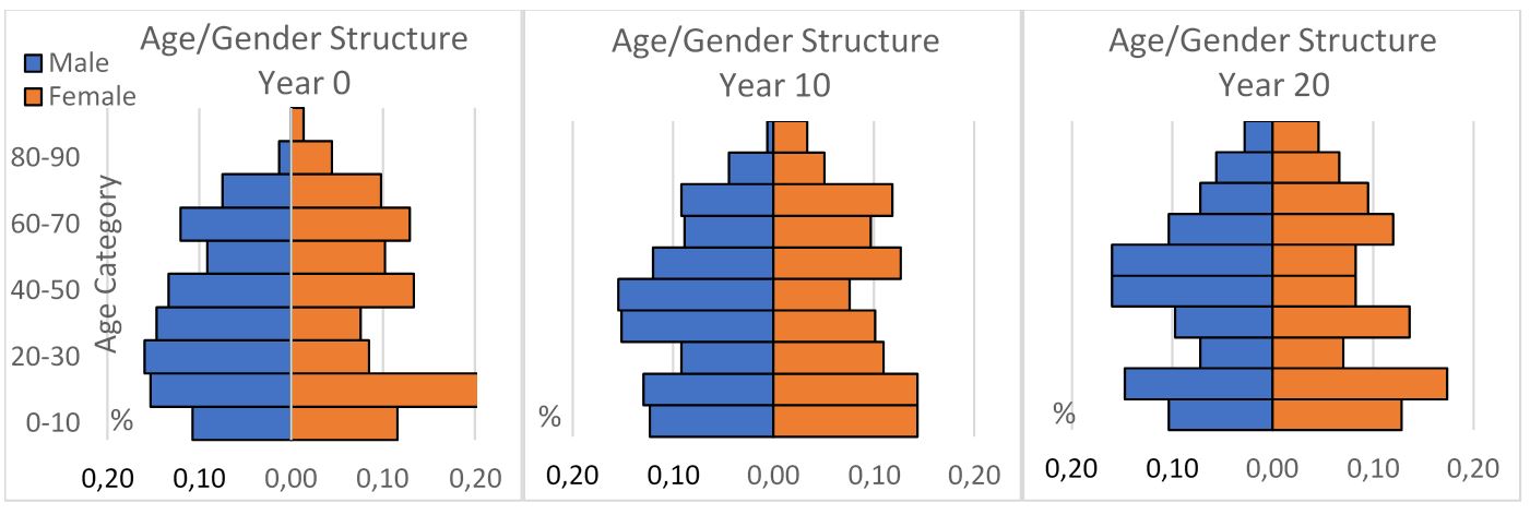
Next, we examine the age and gender structures of the two upper villages at Year 0 (from 2016 survey data), Year 10 (from ABM simulation), and Year 20 (from ABM simulation). We do not have data to validate those in Year 10 (2016) and Year 20 (2036), yet we can take a close look at specific age groups for verification purposes. For instance, the male, 10-20 group is 15% of the total population (left), which turns to be around 7% ten years later (Middle) and 8% 20 years later (right, Figure 3). We explain these decreases using the migration, growth (age-out), and death data: The male group at age 10-20 had 47 people in Year 0, while 0 died and 3 migrated out at Years 0~10. Given that the simulated total population sizes at Years 0~10 are 389, we calculate the percentage of this group at Year 10 to be (47-0-3)/389, or 44/389 = 11.311%, which matches up with the Year 10 bar for males aged 10-20 in Figure 3. Similarly, we explain other percentages in Figure 3.
Third, we examine the projected total area of farmland, which decomposes to GTGP and non-GTGP land area for each of the 94 HHs (Table 2). For verification purposes, we examine land use areas at time 0, time 10, and time 20. The average number and area of non-GTGP parcels both decline with increasing payment, while at the same time the same numbers for GTGP parcels increase. This finding is consistent with literature regarding the impact of payment on PES enrollment (Wunder 2008; Yost et al. 2020).
| Comp. Level* | Steps** | Total # of Non-GTGP Parcels | Total # of GTGP Parcels | Avg. # of Non-GTGP Parcels*** | Avg. # of GTGP Parcels |
| 0 | 6 | 233.27.00 | 143.73.00 | 2.48.00 | 1.53.00 |
| 270 | 6 | 230.93.00 | 146.07.00 | 2.46.00 | 1.55.00 |
| 540 | 6 | 227.90.00 | 149.10.00 | 2.42.00 | 1.59.00 |
| 0 | 732 | 145.00.00 | 232.00.00 | 1.54.00 | 2.47.00 |
| 270 | 732 | 124.47.00 | 252.53.00 | 1.32.00 | 2.69.00 |
| 540 | 732 | 108.10.00 | 268.90.00 | 1.15.00 | 2.86.00 |
| 0 | 1458 | 184.47.00 | 192.53.00 | 1.96.00 | 2.05.00 |
| 270 | 1458 | 182.10.00 | 194.90.00 | 1.94.00 | 2.07.00 |
| 540 | 1458 | 182.50 | 194.50 | 1.94.00 | 2.07.00 |
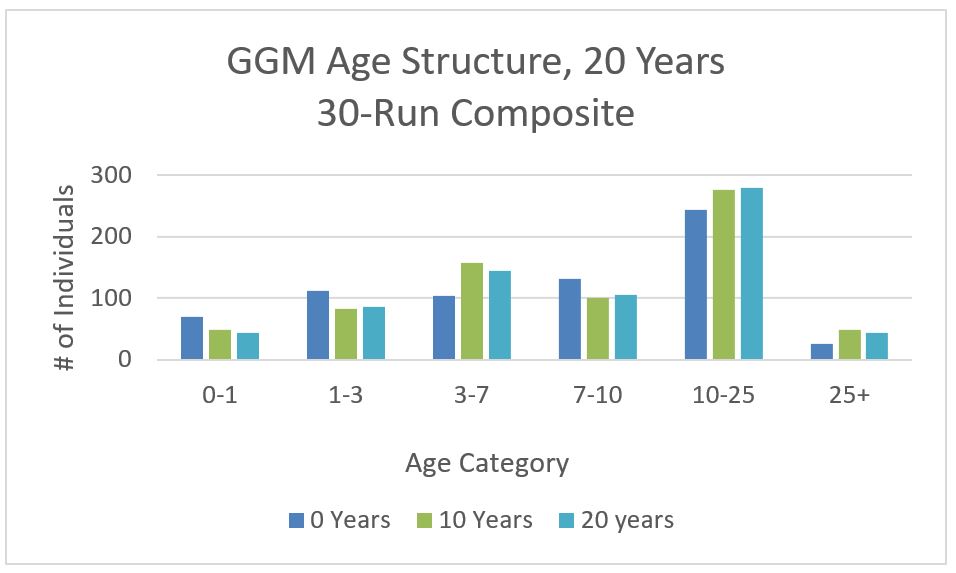
Fourth, we simulate GGM births, deaths, and overall population size from Month #1 to Month #240 (Figure 4). The overall GGM population dynamics (Figure 4a) is consistent with literature (Yang, Lei, & Yang 2002). Yet the overall population dynamics alone may not warrant correctness of processes that constitute such dynamics. For instance, a mistakenly high birth date may offset the impact of a high, yet wrong mortality rate (at some age group) and thus generate “correct” population size, yet giving rise to unbalanced, likely incorrect age structure. Below we examine this potential issue and explore the projected GGM age structure.
We run the ABM and generate GGM age structure (i.e., percent of individuals of 0-1, 1-3, 3-7, 7-10, 10-25 age groups in total GGM population) at Year 10 and 20 (Figure 5). It seems that the two age-structures at Years 10 and 20 are similar to that at Year 0 that is based on literature, yet there are some small differences (e.g., lower % for age 0-1 group and higher % for age 3-7 group). For detailed information and discussion we refer to Mak (2019).
Fifth, we evaluate habitat occupancy using several methods by: 1) presenting the ABM-generated occupancy maps to FNNR managers, seeking their qualitative evaluation of these maps; 2) visually comparing the ABM-generated occupancy maps with a paper habitat map (no digital file) generated from FNNR staff’s long-term fieldwork (Yang, Lei, & Yang 2002); and 3) by comparing occupancy outcomes generated by the ABM (Figure 6) with a small subset of camera-based GGM density data, i.e., only data from the top 11 camera sites (where we have recorded human activity from the 94 households). For each cell, we standardize the GGM occurrence number to a gradient between 0 and 1 by dividing the observed captures by the max captures we have observed there. Then we standardize the ABM predicted occupancy numbers using the same procedure. We calculate the Pearson’s correlation between them. Out of the above three methods, the last one (3) is quantitative, yet subject to several limitations (details in Section Discussion).
The spatial evaluation of habitat occupancy (Figure 6) from experts’ opinions is very positive, suggesting that the overall trend in GGM habitat use has been captured (Y. Yang, personal communication). The qualitative comparison between the FNNR paper map and our ABM-generated map also suggests a good match. The quantitative test gives a moderate result, in which the Pearson’s correlation coefficient is 0.55 (0.69 when a pair of data suspicious of equipment error are removed). We ascribe this to the small sample size (n=11), short term of data collection (1 year) compared to our simulation length (20 years), and equipment bias (e.g., no-detection of GGMs). However, worthy of mention is that the ABM-based occupancy results have been compared to the results from an independent, different modeling approach called MaxEnt, and the results largely match (Mak 2019).
Last, we perform sensitivity analysis using the parameter-sweeping approach (An et al. 2005). In Section 2.11-2.13, the model performance may be sensitive to three parameters, i.e., three radii (centered on a human settlement, farm, and GTGP land parcel) that each define a zone of avoidance by GGMs. We therefore design a GGM-escape test (Table 3). As each parameter has 3 values for test, there are a total of 3x3x3 = 27 experiments. For each experiment, we 1) generate and report habitat occupancy data at the end of simulation and 2) calculate the kappa index between each experiment map and the baseline map at the end of simulation.
Similarly, there is uncertainty regarding minimum amount of cropland that a household hopes to keep and probabilities of enrolling cropland in GTGP or reconverting GTGP land back to cropland (Section GTGP participation and land use). We therefore design a second test named land-decision test (Table 3). As each parameter has 3 values for test, there are also a total of 3x3x3 = 27 experiments under this land-decision test. For each experiment, we collect data regarding 1) the number of GTGP parcels and number of non-GTGP parcels over 20 years (240 months); 2) occupancy data at the end time, and 3) kappa value between experiment occupancy map and baseline occupancy map at the end time.
| Test label | Parameter | Min | Max | Default | Inc** | Outcomes |
| GGM-escape test | Settlement radius | 100 | 700 | 400 | 300 | 1) Occupancy (end) |
| Farm radius (m) | 0 | 600 | 300 | 300 | ||
| Land radius (m) | 0 | 400 | 200 | 200 | 2) Kappa (end) | |
| Land-decision test | Min cropland (Mu) | 0.1 | 0.5 | 0.3 | 0.2 | 1) # of GTGP & non-GTGP parcels over all time steps |
| Prob multiplier 1* | 0.1 | 0.4 | 0.25 | 0.15 | 2) Occupancy (end) | |
Prob multiplier 2* | 0.1 | 0.4 | 0.25 | 0.15 | 3) Kappa (end) |
The above sensitivity analysis results are positive. The two tests do not give any model crash, nor lead to uninterpretable outcomes. The Kappa values in the GGM-escape test have a largely decreasing trend when the threshold (i.e., threshold count for # of steps a cell is used by GGMs: above this value the cell is counted as occupied) increases. The spatial locations of occupied habitat also agree with our experience and experts’ opinion (Appendix B). In land-decision test, the numbers of GTGP-parcels and non-GTGP parcels still converge even when different parameter combinations are used in the model, suggesting that the outcome in (Figure 7) is robust, not likely being an ad hoc outcome (Appendix B).
Experiment design
Once we have evaluated the model and deemed to represent processes in a satisfactory manner, the model is then used to perform scenario experiments. Here we are interested in seeking insights into the impact of GTGP policy on long-term land use, migration, and GGM habitat use. We consider three scenarios: 1) Scenario 1, where GTGP policy stops (payment = 0); 2) Scenario 2, in which GTGP stays as is (payment = 270 Yuan/Mu); and 3) Scenario 3, in which the payment is doubled (payment = 540 Yuan/Mu).
We also examine the potential impact of varying population pressures. In this regard, we design two population scenarios with GTGP payment set at default (270 Yuan/Mu): Scenario 4 features a lower birth plan or fertility rate (1.5 children per woman), in which an eligible woman may have 0, 1, 2, 3, 4, or 5 children in her whole life with a probability of 0.09, 0.5, 0.3, 0.06, 0.03, and 0.02. In contrast, the probabilities are 0.03125, 0.15625, 0.3125, 0.3125, 0.15625, and 0.03125 in the baseline simulation (corresponding to 2.5 children per woman; see Section Human demographics and livelihoods). Scenario 5 features a higher birth plan of 3.5, in which an eligible woman may have 0, 1, 2, 3, 4, or 5 children in her whole life equally with a probability of 0.02, 0.02, 0.04, 0.38, 0.44, and 0.1.
For each of the above scenarios, we intend to estimate the amount of land enrolled in GTGP land (accumulated GTGP land area of 94 HHs), number of accumulated migrants (note that returnee migrants are subtracted), and the related densities of GGMs at FNNR over time. To quantitatively measure the degree of change in GGM occupancy between scenarios, we adopt the Cohen’s kappa statistic that offers an overall agreement (no change in our application) and disagreement (change in our application) on the cell-by-cell basis (Carletta 1996).
Experiment Results
Before we come to our focus regarding the impacts of GTGP policy and population pressure on land use, we briefly examine population trends under different birth plan values. The population size in Year 20 decreases to around 366 under Scenario 4 (BP = 1.5) and increases to around 435 under Scenario 5 (BP = 3.5). The three birth plans do not affect the number of migrants (Figure 2), which may arise from the fact that our time span (20 years) is not long enough for most new births to grow to migration age.
Next, we turn to the impacts of GTGP policy and population pressure on land use (Figure 7). Payment levels do make a big difference in increasing GTGP enrollment in earlier times, e.g., prior to Month 100 (Figure 7a). This finding is consistent with relevant literature, where the positive impact of payment levels on participation has been reported extensively (Wunder 2008; Yost et al. 2020). Yet at later times, some interesting patterns emerge: The non-GTGP land decreases to a nadir, then rises slowly (a concave curve), while the GTGP land rises till a peak is reached, followed by slow decrease (a convex curve). The difference made by the PES payments (or no payment) is the level of increase or decrease and the timing of reaching the peak and nadir. Interestingly, the number of parcels in all three scenarios turns to converge to around two parcels near the end of the 20-years’ time span (we will discuss this finding later). When examining the impact of population pressure, the above convergence pattern is still prevalent at all birth plan values. Yet birth plan values seem to have no impact on land use for the first half of simulation time, and small differences begin to occur at later times: the increase in non-GTGP parcels and decrease in GTGP parcels tend to become slower, resulting in a later convergence time (Figure 7b) .
Worthy of mention is that the above convergence pattern occurs in other parameter settings. As shown in the sensitivity analysis section, this convergence trend also occurs in the 27 experiments with very different parameter values (Appendix B) and is not likely an ad hoc outcome due to this specific parameter setting.

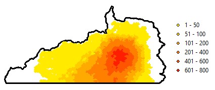
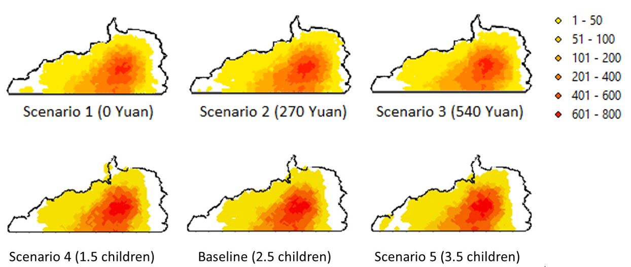
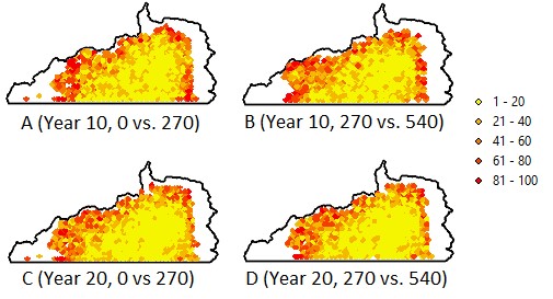
The changes in spatial patterns of habitat use densities are quite informative. When interpreting these maps, it is preferable to reference to (Figure 8), which portrays that the surrounding areas are less used by GGMs. In this context, we can see increasing payment level does improve habitat quality in edge areas, especially areas surrounding the two villages. This arises from local villagers’ resource extraction patterns; mostly they go to nearby areas but do visit remote places occasionally. Therefore, there is no substantial improvement in remote (often core) habitat areas due to a higher GTGP payment. We discuss why this comes out in Section Discussion. Higher or lower fertility rates (birth plans) do not generate big differences in GGM occupancy visually (Scenarios 4 and 5 vs. Baseline; (Figure 8), yet quantitative analysis of Kappa index does show that a decrease in birth plan (from 2.5 to 1.5) makes bigger changes in GGM occupancy more than an increase (from 2.5 to 3.5) does after taking into account the randomness in generating the occupancy measures (Table 8, Appendix C).
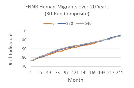
For the northern part of FNNR (our study site) with 94 households, the number of migrants shows a slight, near-linear increasing trend from around 75 to around 105 individuals from 2016 to 2036 (Figure 9; also see Table 1), representing an annual rate of 0.02 person/household. This trend is lower than the general trend between 2000 and 2014 for all the 605 households we surveyed in 2014. There were almost no migrants in 2000 and 340 in 2014, representing an annual rate of increase of 0.04 person per household. This higher rate during 2000 and 2014 is due to the rapid increase near 2002~2005 due to the implementation of GTGP in 2000 (Yang 2019). On the other hand, the payment levels did not change the total number of migrants over time substantially except that stopping payment gives rise to slightly lower number of migrants from Months 49 to 130 (Figure 9).
When evaluating the differences in occupancy due to changes in payment, it appears that compared to the status quo scenario (Scenario 2), the payment level makes a moderate difference in occupancy when threshold is relatively high. When using a threshold of 400 visits/cell (i.e., 20 visits/year; we chose this relatively high value to assure that changes are not by chance, but by substantial changes in GGM visit frequency after consulting experts on GGM ecology and behavior) as a threshold to classify a cell as occupied (a binary classification is required by the Kappa calculation), the Kappa statistic between 0 and 270 payment levels (i.e., Scenarios 1 vs. 2) is 0.8025, while that between 270 and 540 payment levels (i.e., Scenarios 3 vs. 2) is 0.7839. This suggests that changes made by increasing payment are larger than changes (degradation) made by canceling the payment.
Discussion
As reported above, the average number of parcels from model simulations based on all three GTGP scenarios and two population pressure scenarios converges near the end of the 20-year time span (Figure 7). Specifically, GTGP land parcels increase until a peak is reached and then decrease; correspondingly non-GTGP land parcels decrease until a nadir is reached and then increase—this convergence pattern occurs regardless of payment level (Figure 7a). We explain this outcome first by food security. Local households tend to keep a small portion of land unenrolled (i.e., non-GTGP land does not decrease to zero) despite great benefits associated with enrolling in GTGP. During our interviews, respondents repeatedly mentioned this choice, and we translate this choice into a lower bound of non-GTGP land (parameter min cropland in Table 3, default at 0.3 mu). This may reflect the great attraction of labor from local businesses and particularly migration (Zhu 2002).
Interestingly, the convergence pattern occurs regardless of birth plans (fertility rates) as well, and birth plans have little impact on GTGP enrollment, especially at earlier times of simulation (Figure 7b). As household size has a small, positive impact on GTGP enrollment (see Equation 5), an increase in household size due to a larger birth plan (fertility rate) may stimulate the household to enroll more farmland in GTGP, yet other factors such as the above lower bound of non-GTGP land and distance between farmland parcel and household (Equation 5) may stop or dilute this increase in enrollment. For instance, if the increase in household size happens to be in a household with available farmland quite far away, then the tendency in probability increase (due to bigger household size) may be offset by a decrease due to higher household-land distance. Under this condition, capturing spatial heterogeneity (as we did here in terms of mapping all households and their land parcels and thus being able to calculate household-land distances) is very important. Therefore, this surprising convergence pattern is jointly accounted for by the complexity existing in the system (Liu et al. 2008), likely associated with feedback loops and interactions among system components. Although with initial conditions specified by users, any ABM software program could decompose to a set of discrete-time or discrete-event difference equations in principle, such analytical representations become very a dauting task when the system becomes highly complex (Tesfatsion 2017). In this regard, ABM has unique power when addressing questions in complex systems as shown above.
Why does higher GTGP payment increase habitat in edge areas? This finding may arise from the following paths. When GTGP pay increases, the GTGP net cash increases (Equation 3), which will escalate the probability of GTGP participation and simultaneously decrease non-GTGP land. According to Equation 2, a decrease in non-GTGP land will promote out-migration—once people of 15-49 migrate out, local households tend to limit visits to surrounding areas for resource extraction such that GGMs can visit these places at a higher frequency. Again, this finding, though insightful and understandable, is also not one that is intuitive or was expected beforehand. For instance, another potential outcome—GTGP leads to habitat degradation—is possible if this pathway exists: GTGP participation leads to considerable labor released from farming, then local farmers may spend “extra” time extracting local resources for self-use and sale at local markets. However, our data and model results do not support this outcome.
In summary, the merits of this paper lie in the following aspects. First, our research moves forward PES research, which is in nature embedded in both human and environment systems. Participants of PES programs are humans, who make decisions and act in response to various human-environment contexts regulations. Following a set of empirically-established behavioral rules, GGM agents rover on the landscape and respond to changes in the environment, especially human activities. All such processes take place on a spatially explicit landscape, leading to changes in the complex human-environment system. In this context, we have employed a complex systems framework, characterized by an agent-based model that integrates data of varying types, processes or relationships operating at multiple temporal and spatial scales, and knowledge from both natural and social science disciplines.
Our research is innovative in using wildlife (GGM) occupancy as a measure of environmental changes (Scullion et al. 2011), which may be applicable to evaluation of other environmental policies including PES. In addition, movement analysis and modeling is a hot topic in space-time analysis and animal behavioral ecology (An et al. 2015; Tang & Bennett 2010). Our semi-random walk approach—in the context of human disturbance—may provide better understanding of animal behavior. Furthermore, our agent-based modeling practice contributes to ABM testing (e.g., using structural measures such as age structure, parameter sweeping test), model transparency and reusability (all code in the CoMSES repository), and modeling of human decision—a daunting challenge that attracts increasing recognition in many simulation and modeling (including ABM) domains. Such contributions may help advance complexity science (Manson 2001), addressing the YAAWN syndrome in the ABM arena (O’Sullivan et al. 2016) and many other challenges in the ABM domain (An et al. 2017).
Caveats arise concerning spatial and temporal resolutions. In our model, the temporal resolution is 5 days, while resource collection takes place on a daily basis. This mismatch (1-day vs. 5-day time step) has forced us to spread the 1-day influence into a 5-day period (see Section Resource extraction). This may bias the simulated influence of human visits on GGM habitat use, especially the temporal dimension of such influence. In the future, a finer temporal resolution (e.g., daily or even hourly) should be tested if simulation speed is not sacrificed much, or parallel or cloud computing techniques can be employed. A similar issue is for the relatively coarse spatial resolution (near 300 m). In the future, a 30 m spatial resolution may be adopted, which enables us to map GGM and human activities on a more precise basis.
Also worth of mention is the moderate quality of spatial projections about GGM occupancy. Although able to capture generic trends of GGM habitat use, the model results are not in high agreement with our observed camera-trap data. In addition to the reasons mentioned above (low sample size, short term of data collection, and equipment bias), we also offer one important reason: The spatial locations of cameras, subject to human accessibility, are not very representative of all GGM accessible habitat areas. At such human-accessible locations, collection of human activity data may be more challenging due to reasons such as local people’s unwillingness to share their activities or spatial inaccuracy when mapping human activities.
Conclusion
This paper aims to reveal complex, reciprocal relationships among PES, human livelihoods, and the environment (both land use and land cover and habitat occupancy) at Fanjingshan National Nature Reserve, China. The agent-based model contributes to integrating data from different spatial and temporal scales and disciplines, revealing land use and habitat patterns that are difficult to obtain otherwise. Instead of being used as a predictive tool, we recommend that our model be used as a platform to study and further understand complex human-environment systems, shedding light on key elements, interactions, or relationships in such systems. Efforts in this regard will help us establish PES science that incorporates features in complex systems, such as heterogeneity, feedback, and nonlinearity, offering more realistic, spatially and temporally explicit scenarios related to human policy or intervention. All these contribute to achieving the United Nations’ 17 Sustainable Development Goals (United Nations 2016), especially Goal 15 that aims to protect, restore and promote sustainable use of terrestrial ecosystems.
Acknowledgements
This research was funded by the National Science Foundation under the Dynamics of Coupled Natural and Human Systems program [DEB-1212183 and BCS-1826839]. This research also received financial and research support from San Diego State University. We thank Fanjingshan National Nature Reserve in China, Research Center for Eco-Environmental Sciences at the Chinese Academy of Sciences, and Yunnan University for logistic support.Model Documentation
The model was built in Phyton with MESA and is fully accessible here: https://www.comses.net/codebases/0852f2b8-6517-4b83-b7fa-8304eb538421/releases/1.0.0.Notes
- According to an online survey, the numbers of articles and authors reporting the development or use of ABMs have risen steadily in an exponential rate since the mid-1990s, covering a wide range of disciplines (An, Volker, & Turner 2020)
- In 2018 FNNR has been approved to a World Natural Heritage Site, and its territory will likely be expanded (Shi personal communication).
- Such groups consist of males aged 10-25 that have migrated out from original groups.
- The lower bound could be 1300 m (Bleisch, Long, & Richardson 2008) and even 570 m in extreme situations (Niu, Tan, & Yang 2010).
- This and other two radii are based on personal communications with expert in GGM behavior, Mr. Yeqin Yang (February 28~March 1, 2019). They are parameters subject to changes. See Section Model evaluation for our sensitivity test following An et al. (2005).
- There is a small chance that two people within the two villages may marry, thus not bringing in a person from outside. As the probability is very small according to An et al. (2005), we overlook this to simplify the model.
- If a returnee migrant comes back, then s/he is not considered as migrant.
Appendix
The ODD (Overview, Design concepts, & Details) Protocol for an agent-based model is a standardized document which outlines a model’s purpose, variables, framework, schedule, and data. The format was conceptualized by a team of twenty-eight authors who had previously published or worked with agent-based models, and serves as a universal set of guidelines for describing a model (Grimm et al. 2006; Grimm et al. 2010).
A: ODD protocol
Purpose
This agent-based model serves a variety of inter-connected purposes:
- To simulate the demographic changes of humans living in the FNNR, including births, deaths, marriages, out-migration and re-migration. These changes are modeled on the existing human data gathered from the FNNR. Heads of household are also designated. Various other statistics, such as income level and education level, are projected as well. Finally, human age structures are recorded.
- To simulate GGM movement within the FNNR in a movement sub-model, which follows seasonal patterns of migration to a mating area and avoids human settlements or low elevations. Movement is also weighted according to the nearby vegetation: monkeys are more likely to move to vegetation that they are modeled to favor.
- To simulate human resource collection in the movement sub-model, which may impact the movement of humans upon GGM habitat.
- To simulate Green-to-Grain Program (GTGP) enrollment or dis-enrollment and GTGP land conversion, which is based on factors such as current income and types of land owned.
- To simulate the demographic changes of the Guizhou Golden Monkey (referred to henceforth as GGM) of the Fanjingshan National Nature Reserve (referred to henceforth as FNNR) over time, including births, deaths, formation of new families from a large group or of all-male groups, and mating behavior. Monkey demographic (age and gender) structures are also recorded.
Entities, State Variables, & Scales
Time - Each time-step of the model represents approximately 5 days. Therefore, every 73 steps of the model, the model “advances” one year. Individual processes such as birth, death, and adulthood are continuous, and may occur at any time-step once conditions are met. While not an entity in itself, the passage of time will trigger events, such as birth or the formation of new groups.
| Entity | State Variables & Attributes | Spatiotemporal Scales & Extents |
| Guizhou Golden Monkey (individual agents in mostly-stacked collective) Monkeys are defined by families in the visualization submodel and by individuals in the population submodel. | Unique ID Age Age Category Gender Birth Interval Family ID Family Size Mother ID Current Position Past Position Family Type Split Flag (if families grow too large) | Spatial: One pixel represents a family group of 20-50 monkeys, which move together. Temporal: Monkeys have a lifespan of approximately 30 years. At 8 years, they become adults and can begin to mate. |
| Human (stacked collective, single moving agents) In the movement model, only heads of households move to collect resources. | Unique ID Age Gender Education Work Status Marriage Status Household ID Past HH ID (if migrated) Home Location Migration Status # of Migrated Years Migration Network Migration Remittances Resource Location Resource Frequency Current Position GTGP Participation (Household) GTGP Area (mu, Household) Off-Farm Income (Household) | Spatial: One pixel represents a non-moving household, each of which has zero or one human agents who is a fuelwood collector and a varying number of total human agents within it. Any human agents that travel will always return to their household pixel. Temporal: Like monkeys, humans age, sometimes reproduce, and die. Their lifespan and other variables are set in the model. |
| Environment (grid cell) Potential Subtype: Household, Farm, PES, (Managed) Forest | Elevation Vegetation Type | Spatial: The extent of the FNNR. Elevation is adapted from 30m raster DEMs, scaled down by 10 to create a manageable grid. The sq. area of the rectangular grid containing the FNNR extent—that is, not the FNNR itself—is approximately 640 sq. km. One environmental grid cell represents approximately 275m in diameter, or 0.075 sq. km in area. Temporal: None, though the agents interact with the environment by avoiding areas of low or high elevations. |
Land (GTGP Area; not shown in movement model) | Unique ID Household ID GTGP Participation GTGP Land Area (mu) GTGP Net Income (yuan) Total Land Income Head-of-Household Age, Gender, & Education Level Land Type (rice or dry) Land Travel Time Plant Type Household Size GTGP Dry Land Area (mu) GTGP Paddy Land Area (mu) Total Dry Area (mu) Total Rice Area (mu) Non-GTGP Output (yuan) Pre-GTGP Output (yuan) Non-GTGP Area (mu) Unit Compensation | Spatial: None Temporal: Every step, there is a small chance GTGP conversion will be checked. If it is checked, then there is a chance that a land parcel may convert to a GTGP or non-GTGP land parcel, which will affect household-level variables such as income or land type. This chance is based on a regression formula that includes factors such as land type, current household income, and unit compensation. |
Process Overview & Scheduling
All agents move in a random order, which does not affect the processes within each step. The processes are carried out in the same order for every agent; for example, for individual monkey agents, the death check always occurs at the end of every step. Possible agent actions, which may be restricted by certain agent attributes such as gender or age, are as follows:
- Model (Step 0 only): Create GGM family agents, monkey agents belonging to each family, human agents, land agents that refer to household-level lists that humans access, resource agents, and environmental grids
- Land Parcels (each step, land submodel only): simulate GTGP conversion, update household income, update GTGP area changes from conversion
- Humans (each step, movement/visualization submodel only): Head to resources, gather resources, head back to house, and randomly select another resource to gather
- GGM Family (each step, movement submodel only): Avoid humans if paths cross, avoid areas of low or high elevation (seasonally), move to Yangaoping (breeding site), move away from Yangaoping, and move to neighboring cells according to a correlated random-walk (path determined by vegetation and elevation) as described by Ahearn et al. (2016).
- GGM Individual (each step, population submodel only): Age, possibly give birth (if female and of age), possibly out-migrate to another group (depending on age, gender, and current group size—male monkeys may defect to an all-male group, and large families can split into smaller groups), and die
- Human Individual (each step, population submodel only): Age, possibly give birth (if female and of age), possibly marry, possibly out-migrate (sometimes in a special case due to college, where they typically do not re-migrate from) and re-migrate, gain education levels, change work status, possibly change head-of-household status, and die
Design concepts
Discussed here are the eleven design concepts of the ODD protocol: basic principles, emergence, adaptation, objectives, learning, prediction, sensing, interaction, stochasticity, collectives, and observation (Grimm & Railsback 2005).
Basic principle
Visualization submodel – This assumes spatial patterns among all GGM families, such as yearly migration to Yangaoping; movement patterns are also calibrated according to movement needs as determined by known travel speeds, vegetation preferences, and behavior around humans from the literature (Grimm and Railsback 2005, Yang, Lei, & Yang 2002). Because the model input is directly based on observations from a field study, the default output—a showcase of movement over ten years—is expected to be fairly predictable. What is new about this model is the comparison of its output—a point density map of its movements—to a Maxent model through Cohen’s Kappa, and a discussion of how different versions of this model—based on configuration settings such as GTGP unit compensation—may differ through a similar comparison.
Population submodel – This confirms GGM population structure observations from Yang, Lei, & Yang’s field study (2002) by modeling changes to the population over ten years based on birth, mortality, and birth-interval rates per age category. It does not consider intermediate factors that are not currently well-understood by the literature, such as low genetic diversity and the impact of this phenomenon on birth defects or miscarriages, or whether or not closely-related monkeys can breed. However, it considers the observed patterns of male departure from groups and refreshed fertility after a recent loss of an infant. The population submodel also assumes a stable human age demographic, stable migration, and consistent birth, death, and marriage rates in relation to China’s national averages.
GTGP conversion submodel – This assumes that households will enroll in GTGP given that they meet a certain threshold as determined by the regression formula, and that they are likely to revert after a number of years without compensation after the program ends.
Emergence
Visualization submodel – Avoidance of humans and human settlements may have more or less of an impact than expected; vegetation weights may more or less than an impact than expected.
Population submodel – Fertility “recovery” after loss of an infant may have more or less of an impact than expected.
GTGP conversion submodel – GTGP unit compensation may have more or less of an impact than expected; the model also does not account for any land area changes as a result of GTGP enrollment in the visualization submodel.
Adaptation
Visualization submodel – Family agents avoid less-desirable cells with human settlements and lower elevations, and choose their neighboring cell by weights determined by vegetation type.
Population submodel – Fertility “recovery” or the lessening of between-birth intervals, after the loss of an infant is an adaptive trait that female individuals may have.
GTGP conversion submodel – GTGP enrollment affects income and GTGP land area, which plays a role in future GTGP enrollment.
Objectives
Visualization submodel – GGM Family agents primarily avoid humans, move to ideal vegetation, and visit Yangaoping for breeding and giving birth. The human agents’ only objective is to gather resources and return to their homes.
Population submodel – Adaptations—and therefore objectives—are more chance-based rather than individual-objective based. For example, human and GGM agents have a small chance of dying every step, which cumulates to a yearly mortality rate every 73 steps.
GTGP conversion submodel – Adaptations—and therefore objectives—are more chance-based rather than individual-objective based. For example, land parcels have a chance of conversion and adjusting household income every step.
Learning
This model does not have agents change their traits responsively as part of its process, but can be modified to do so using “self” variables. The closest feature it has is using the outputs of processes, such as increased income from GTGP conversion, to inform other future decisions.
Prediction
Agents do not estimate future consequences of decisions; decisions made are based on information available at the time, and often impact current decisions immediately thereafter, or on a cumulative basis.
Sensing
Visualization submodel – GGM Family agents sense the presence of humans gathering resources and human settlements, and will move so as not to overlap them. They also “sense” the vegetation and elevation around them.
Population submodel – Female monkey agents give birth at the correct ages, and if male, may migrate to other groups.
GTGP conversion submodel – Income and land parcel interaction affect each other, so higher temporary income may result in lower GTGP enrollment, which creates a negative feedback loop (lower GTGP enrollment may also temporarily lower income).
Interaction
Visualization submodel – Humans gather resources, but otherwise do not interact with GGMs. The model may be changed later, e.g. to implement a poaching behavior.
GGMs avoid humans, and will not move to occupy the same or sometimes even an adjacent pixel (each pixel is a ~300-meter space) as a human agent.
Population submodel – if any monkey infant dies, its mother may give birth again the following year (a “recovery” of fertility), even though the normal birth interval rate is 3 years. Humans will gather resources less efficiently if they are marked as a resource-gathering household, but the head of the household/workers of age are currently migrated or die without a replacement.
GTGP conversion submodel – increased household income from GTGP conversion may result in higher out-migration rates; the end of the PES program will cause some households to revert their GTGP-enrolled land parcels.
Stochasticity
Visualization submodel – GGM agents move to their 8-cell (diagonal and adjacent) neighbors according to a weighted choice, which in turn is informed by the vegetation type of each neighbor. Males can also travel between groups or form an all-male group when of a sufficient age.
Population submodel – For both monkey and human agents, births and deaths are random chances determined by a birth-interval rate or yearly rate.
GTGP conversion submodel – A weighted-probability-based formula decides whether or not a land parcel converts to GTGP, which in turn affects human household income.
Collectives
In both the movement and population submodels, GGM individuals belong to a family; occasionally, all-male families can break off.
Land parcels belong to a household collective, which humans also belong to; the collective is accessed via lists, so there are no household agents.
Observation
The output of the movement model is a .csv file of all points that individual agents traveled to, from which a heatmap or point density map may be generated.
The output of the population submodel are .csv files tracking changes in the population and age/sex structure over time.
The output of the GTGP conversion submodel is a .csv file of non-GTGP and GTGP land parcel counts, areas, and household income tracking.
Initialization
All initial values for humans and GGMs are either taken from Yang, Lei and Yang's 2002 field study of the GGMs (in the case of population structure rates), or from data which was gathered as part of the greater FNNR project (in the case of environmental, resource, or human household data).
Visualization submodel – Initial settings (number of years the model runs for, number of monkey families, GTGP compensation structure, PES program span, etc.) are set by the user in fnnr_config_file.py before running the model.
Population submodel – Each family group contains 25-45 agents, and in total, there are between 600-900 monkeys in the reserve (very likely 650-750).
GTGP conversion submodel – Income is determined at the start by current land income and off-farm income combined. Some land parcels are already enrolled in GTGP.
Input data
| Entity | Input Data | Data Source |
| Guizhou Golden Monkey | Seasonal movement behavior (qualitative), birth rates, death rates, birth-interval rates, group-migration or infant-loss behavior (qualitative) | Field study (Yang, Lei, & Yang 2002), other literature |
| Humans | Household locations, birth rates, death rates, marriage rates, education rates, regression factors for migration probability, income levels, age/work status/gender/education levels for current FNNR residents | FNNR Project at SDSU |
| Resources | Resource location Resource type | FNNR Project at SDSU |
| Environment | Vegetation map DEM (digital elevation model) | FNNR Project at SDSU; vegetation categories map and DEM processed by Tsai (2016) |
| Land Parcel | Regression factors for GTGP conversion, current area/land type/land travel time for current FNNR land parcels | FNNR Project at SDSU |
Submodels
The processes for the three submodels are outlined here. Step 0 – all agent and environment types (families, individual monkeys, humans, resources, land parcels, environment) are parametrized and created.
Visualization submodel ordered priorities for GGM family agents:
- Avoid humans and human settlement buffers (cannot enter certain occupied cells or face lower random odds of entering weighted cell).
- Head to or from Yangaoping if it is directly before, during, or after mating season or birthing season (e.g. September, or steps 46-55 in a year of 73 steps).
- Avoid certain low or high elevations. If traveling to or from Yangaoping, they may temporarily pass through those cells.
- Move to neighboring cells (usually 5-10 times in a step to match the distances covered over five days, or one step, as noted in the literature) based on a random choice affected by weights assigned to each neighbor, which in turn is determined by one of nine vegetation types: mixed, broadleaf, deciduous, conifer, bamboo, shrublands, lichen, clouds (usually random; artifact from classification process), or farmland.
Visualization submodel ordered priorities for human agents:
- If at home, choose a random resource from an imported list of resources their household gathers, and head towards the resource in a shortest-distance path.
- Once at the resource, head back home to deposit the resource, and repeat the process.
- Since humans gather resources faster than the time resolution of the model (one time-step represents 5 days), the visualization will show human agents “jumping” back and forth between resources up to each step; however, the coordinates traveled along the paths are recorded.
Population submodel for GGM individuals:
- Face a low-level mortality rate each five-day step (slightly less than the yearly mortality rate divided by 73, since 73 * 5 = 365 days in one year, because of compounding probability). Mortality rates differ by age category.
- If female and of age, birth interval increases every step; if it exceeds 3 (with no recent infant loss), give birth. If it exceeds 1 (recent infant loss), also give birth. Once a female has given birth, their birth interval resets to 0, and builds up again over time.
- If male and of age, and if enough are “flagged” by a low-level chance once they reach of age, an all-male group may break off, and males will change families.
- Each step, population dynamics are recorded (in some versions of the model; other versions only record the first and last step), and at the final step (ten years = 730 steps; twenty years = 1460 steps), a .csv file is generated. This file includes the starting/ending population and average age/sex structure of the population.
Population submodel for Human individuals:
- Face a low-level mortality rate each five-day step (slightly less than the yearly mortality rate divided by 73, since 73 * 5 = 365 days in one year, because of compounding probability).
- Every step, there is a low chance a new baby will be born. If that chance is met, a random married female who has not given birth in the last two years will be selected to bear a child, and the household size will increase. Once a female has given birth, their birth interval resets to 0, and builds up again over time.
- If single and of age, there is a low chance of marriage occurring every step. Divorce is not accounted for in the model.
- Miscellaneous variables such as education and work status update semi-randomly depending on other weighted factors such as the person’s age.
- Humans may migrate out or re-migrate back if they have migrated. These are based on regression formulas that consider gender, age, income, migration networks, ratio of land owned to laborers in the household, and education level.
- Migration changes who is designated as the head of the household, which may in turn impact resource gathering (alternative heads of households, especially if not of age, may gather resources more slowly).
- Each step, population dynamics are recorded (in some versions of the model; other versions only record the first and last step), and at the final step (ten years = 730 steps; twenty years = 1460 steps), a .csv file is generated. This file includes the starting/ending population and average age/sex structure of the population.
GTGP conversion submodel:
- Each step, a small probability for GTGP enrollment or dis-enrollment is evaluated for each land parcel. This is based off a formula that considers the head of the land parcel’s household’s gender, age, education, and income. It also considers the time taken to travel to the parcel from the household, the land type, and the number of humans in the household (household size).
- Non-GTGP land area, GTGP land area, and household income (for all land parcels of that household) are updated to reflect changes from GTGP enrollment.
Appendix B: Sensitivity analysis results
Sensitivity design
The sensitivity analysis is comprised of two tests: the Guizhou golden monkey (GGM) escape test (or GGM-escape test) and the land-decision test. For detail of the test design, see Section Model evaluation and Table 3 in the main text.
Results of GGM-escape test
Below is the GGM habitat occupancy under the GGM-escape test, in which three radii (centered on a human settlement, farm, and GTGP land parcel) are exposed to sensitivity test. Note that each radius defines a zone of avoidance by GGMs. For each scenario or parameter setting, the simulation is run 30 (or 10 depending on the scenario) times with results collected and saved in a certain directory. Once all simulation results are collected, we calculate values of several key variables such as human population size, # of migrants, number of GTGP or non-GTGP parcels, etc.
| Threshold count (TC) for # of steps a cell is used by GGMs: above this TC the cell is counted as occupied | Kappa Average for other 29 combos vs. 0.25-0.25-0.3* | Kappa Average at baseline (0.25-0.25-0.3) scenario** |
| 50 | 0.9184 | 0.9181 |
| 100 | 0.9267 | 0.9265 |
| 200 | 0.8790 | 0.9006 |
| 400 | 0.7712 | 0.7837 |
| 600 | 0.5948 | 0.6348 |
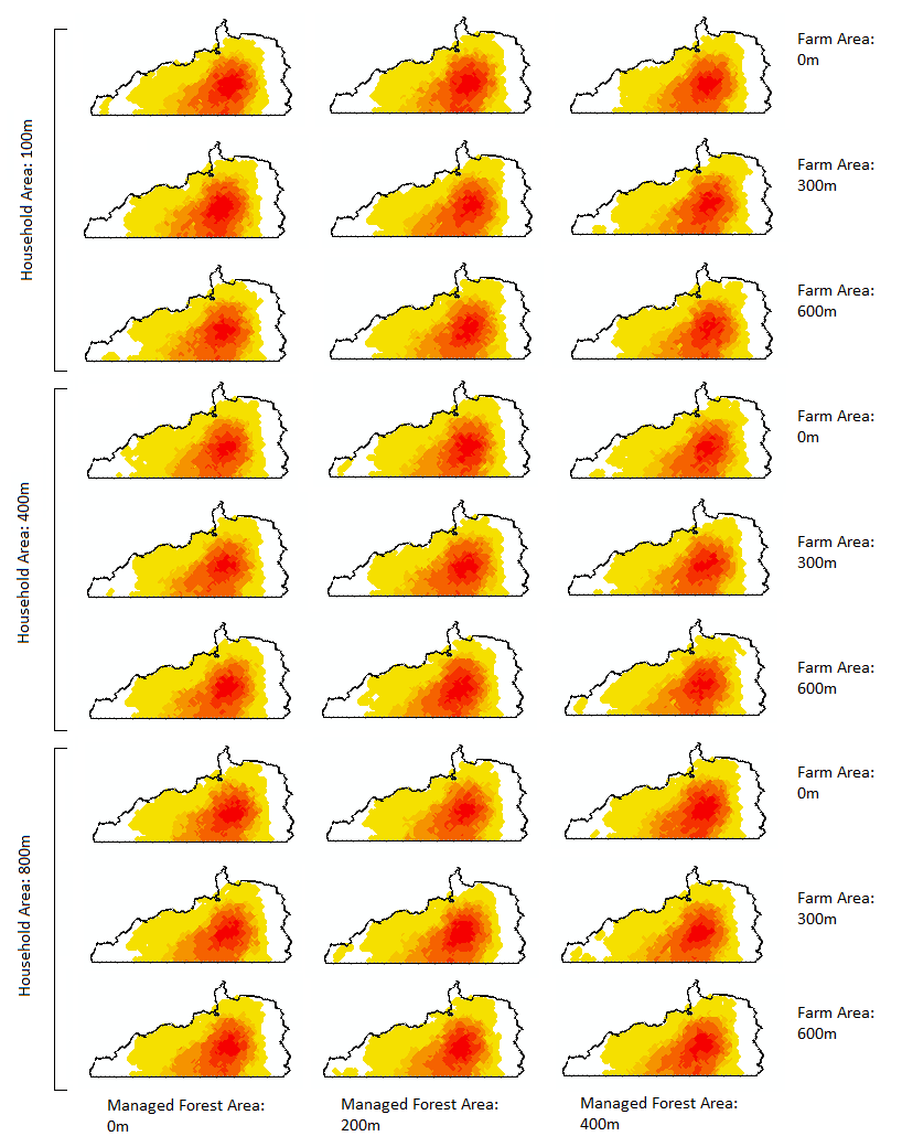
Visually comparing maps for spatial locations of habitat occupancy (Figure 11), we do not see big differences due to the three parameters. Then we turn to examine the Kappa values. It appears that the model is not very sensitive to changes in the three parameters settlement radius, farm radius, and land radius (Table 6) given the magnitudes of Kappa index among baseline results (the right column in Table 6). When the threshold increases from 50 to 600, the differences in Kappa between a certain GGM-escape test and the baseline tend to increase as well.
Results of land-decision test
From the dynamics of the number of GTGP parcels and that of non-GTGP parcels, we can see that the converging trend still exists (Figure 12). Note that we sweep the three parameters min cropland (Mu), probability multiplier 1, and probability multiplier 2 at values specified in Table 3 of the main text.
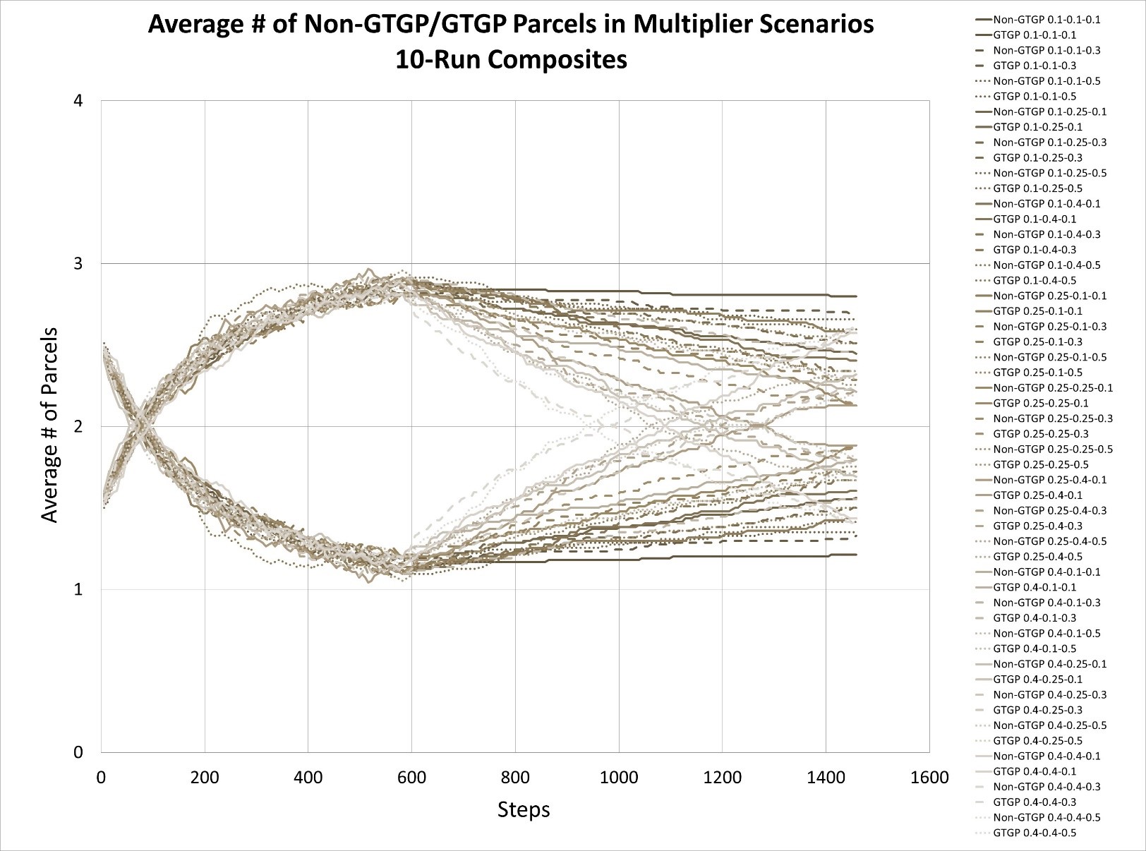
Below we show the differences in Kappa due to changes in the three parameters of min cropland (mu), probability multiplier 1, and probability multiplier 2 (Table 7). Comparisons between two Kappa values at the same threshold show that changes in the three parameters give small-to-moderate changes in habitat occupancy.
| Threshold count (TC) for # of steps a cell is used by GGMs: above this TC the cell is counted as occupied | Kappa Average for other 26 combos vs. baseline (400m-300 m-200 m)* | Kappa Average at baseline (400 m-300 m-200 m) scenario ** |
| 50 | 0.9226 | 0.9181 |
| 100 | 0.9259 | 0.9265 |
| 200 | 0.8930 | 0.9006 |
| 400 | 0.7705 | 0.7837 |
| 600 | 0.6104 | 0.6348 |
Appendix C: Kappa analysis results for population scenarios
Here we present the Kappa analysis results showing the occupancy differences between different birth plan (fertility rate) scenarios (Table 8). As the average Kappa among baseline simulation results is around 0.63 (Table 6), it seems that changing birth plan to a higher or lower value does affect habitat occupancy in the long run.
| Threshold count (TC) for # of steps a cell is used by GGMs: above this TC the cell is counted as occupied | Scenario 4 (1.5 BP*) vs. Baseline (2.5 BP) (30 Run Comparisons) | Scenario 5 (3.5 TFR) vs. Baseline (2.5 BP) (30 Run Comparisons** |
| 50 | 0.9193 | 0.9189 |
| 100 | 0.9309 | 0.9300 |
| 200 | 0.8872 | 0.8931 |
| 400 | 0.7706 | 0.7785 |
| 600 | 0.5882 | 0.5754 |
References
ADHIKARI, B., & Agrawal, A. (2013). Understanding the social and ecological outcomes of PES projects: A review and an analysis. Conservation and Society, 11(4), 359–374. [doi:10.4103/0972-4923.125748]
AHEARN, S.C, Somayeh, D., Simcharoen, A., Glenn, X., & Smith, J. (2016). A context-sensitive correlated random walk: A new simulation model for movement. International Journal of Geographical Information Science, 31(5): 867-883. [doi:10.1080/13658816.2016.1224887]
AN, L. (2012). Modeling human decisions in coupled human and natural systems: Review of agent-based models. Ecological Modelling, 229, 25–36. [doi:10.1016/j.ecolmodel.2011.07.010]
AN, L., Linderman, M., Qi, J., Shortridge, A., & Liu, J. (2005). Exploring complexity in a human-environment system: An agent-based spatial model for multidisciplinary and multiscale integration. Annals of the Association of American Geographers, 95(1), 54–79. [doi:10.1111/j.1467-8306.2005.00450.x]
AN, L., Manson, S., Jankowski, P., Wang, S., & Turner II, B. L. (2017). (NSF proposal) ABM’17: The usefulness, uselessness, and impending tasks of agent-based models in social, human-environment, and life Sciences. Retrieved from https://www.nsf.gov/awardsearch/showAward?AWD_ID=1638446&HistoricalAwards=false
AN, L., Tsou, M.-H., Crook, S., Chun, Y., Spitzberg, B., Gawron, J. M., & Gupta, D. (2015). Space-time analysis: Concepts, quantitative methods, and future directions. Annals of Association of American Geographers, 105(5), 891–914. [doi:10.1080/00045608.2015.1064510]
AN, L., Volker, G., & Turner, B. L. II. (2020). Editorial: Meeting Grand Challenges in Agent-Based Models. Journal of Artificial Societies and Social Simulation, 22(1), 3: https://www.jasss.org/23/1/13.html.
AN, L., Zvoleff, A., Liu, J., & Axinn, W. (2014). Agent based modeling in coupled human and natural systems (CHANS): Lessons from a comparative analysis. Annals of Association of American Geographers, 104(4), 723–745. [doi:10.1080/00045608.2014.910085]
ASSESSMENT, M. E. (2005). Ecosystems and Human Well-Being. Washington, DC: Island Press.
AXELROD, R., & Cohen, M. D. (1999). Harnessing Complexity: Organizational Implications of a Scientific Frontier. New York: The Free Press.
BLEISCH, W., Cheng, A.-S., Ren, X.-D. & Xie, J.-H. (1993). Preliminary results from a field study of wild Guizhou snub-nosed monkeys (Rhinopithecus brelichi). Folia Primatologica, 60(1–2), 72–82. [doi:10.1159/000156677]
BLEISCH, W., Long, Y.-C., & Richardson, M. (2008). Grey snub-nosed monkey. Retrieved from The IUCN Red List of Threatened Species website.
CARLETTA, J. (1996). Assessing agreement on classification tasks: The Kappa statistic. Computational Linguistics, 22(2), 249–254.
CHEN, H. L., Lewison, R., An, L., Tsai, Y. H., Stow, D., Shi, L., & Zhang, W. (2020). Assessing the effects of payments for ecosystem services programs on forest structure and species biodiversity. Land Use Policy, under review.
CLAASSEN, R., Cattaneo, A., & Johansson, R. (2008). Cost-effective design of agri-environmental payment programs: U.S. experience in theory and practice. Ecological Economics, 65(4), 737–752. [doi:10.1016/j.ecolecon.2007.07.032]
Council, N. R. (2014). Advancing Land Change Modeling: Opportunities and Research Requirements. Washington, DC: The National Academies Press
CURRAN, L. M., Trigg, S. N., McDonald, A. K., Astiani, D., Hardiono, Y. M., Siregar, P., … Kasischke, E. (2004). Lowland Forest Loss in Protected Areas of Indonesian Borneo. Science, 303(5660), 1000–1003. [doi:10.1126/science.1091714]
DAILY, G. C., & Matson, P. A. (2008). Ecosystem services: from theory to implementation. Proceedings of the National Academy of Sciences of the United States of America PNAS, Proceedings of the National Academy of Sciences, 105(28), 9455–9456. [doi:10.1073/pnas.0804960105]
ENGEL, S. (2016). The devil in the detail: A Practical guide on designing payments for environmental services. International Review of Environmental and Resource Economics, 9, 131–177. [doi:10.1561/101.00000076]
FRIESS, D. A., Phelps, J., Garmendia, E., & Gómez-Baggethun, E. (2015). Payments for Ecosystem Services (PES) in the face of external biophysical stressors. Global Environmental Change, 30, 31–42. [doi:10.1016/j.gloenvcha.2014.10.013]
GDF, & FNNR. (1990). The Study of Fanjingshan (Guizhou Department of Forestry and Fanjingshan National Nature Reserve Administration). Guiyang, China: Guizhou People Press.
GRIMM, V., Berger, U., Bastiansen, F., Eliassen, S., Ginot, V., Giske, J., Goss-Custard, J., Grand, T., Heinz, S. K., Huse, G., Huth, A., Jepsen, J. U., Jørgensen, C., Mooij, W. M., Müller, B., Pe’er, G., Piou, C., Railsback, S. F., Robbins, A. M., Robbins, M. M., Rossmanith, E., Rüger, N., Strand, E., Souissi, S., Stillman, R. A., Vabø, R., Visser, U. & DeAngelis, D. L. (2006). A standard protocol for describing individual-based and agent-based models. Ecological Modelling, 198(1–2), 115 – 126. [doi:10.1016/j.ecolmodel.2006.04.023]
GRIMM, V., Berger, U., DeAngelis, D. L., Polhill, J. G., Giske, J. & Railsback, S. F. (2010). The ODD protocol: A review and first update. Ecological Modelling, 221(23), 2760–2768 [doi:10.1016/j.ecolmodel.2010.08.019]
GRIMM, V. & Railsback, S. F. (2005). Individual-Based Modeling and Ecology. Princeton, NJ: Princeton University Press.
HE, J., & Sikor, T. (2015). Notions of justice in payments for ecosystem services: Insights from China’s Sloping Land Conversion Program in Yunnan Province. Land Use Policy, 43, 207–216. [doi:10.1016/j.landusepol.2014.11.011]
IRWIN, E. G., & Geoghegan, J. (2001). Theory, data, methods: Developing spatially explicit economic models of land use change. Agriculture, Ecosystems and Environment, 85(1), 7–24. [doi:10.1016/s0167-8809(01)00200-6]
LEVIN, S., Xepapadeas, T., Crépin, A.-S., Norberg, J., De Zeeuw, A., Folke, C., Hughes, T., Arrow, K., Barrett, S., Daily, G., Ehrlich, P., Kautsky, N., Mäler, K.-G., Polasky, S., Troell, M., Vincent, J. R. & Walker, B. (2013). Socialecological systems as complex adaptive systems: Modeling and policy implications. Environment and Development Economics, 18(02), 111–132. [doi:10.1017/s1355770x12000460]
LEWISON, R. L., An, L., & Chen, X. (2017). Reframing the payments for ecosystem servicesframework in a coupled human and naturalsystems context: strengthening the integrationbetween ecological and human dimensions. Ecosystem Health and Sustainability, 3(5). [doi:10.1080/20964129.2017.1335931]
LIU, J., & Diamond, J. (2005). China’s environment in a globalizing world: How China and the rest of the world affect each other. Nature, 435(7046), 1179–1186. [doi:10.1038/4351179a]
LIU, J., Dietz, T., Carpenter, S. R., Alberti, M., Folke, C., Moran, E., … Taylor, W. W. (2007a). Complexity of coupled human and natural systems. Science, 317(5844), 1513–1516. [doi:10.1126/science.1144004]
LIU, J., Dietz, T., Carpenter, S. R., Folke, C., Alberti, M., Redman, C. L., … Provencher, W. (2007b). Coupled human and natural systems. AMBIO: A Journal of the Human Environment, 36(8), 639–649. [doi:10.1579/0044-7447(2007)36[639:chans]2.0.co;2]
LIU, J., Li, S., Ouyang, Z., Tam, C., & Chen, X. (2008). Ecological and socioeconomic effects of China’s policies for ecosystem services. Proceedings of the National Academy of Sciences, 105(28), 9477–9482. [doi:10.1073/pnas.0706436105]
LIU, J., Linderman, M., Ouyang, Z., An, L., Yang, J., & Zhang, H. (2001). Ecological degradation in protected areas: The case of Wolong nature reserve for giant pandas. Science, 292(5514), 98–101. [doi:10.1126/science.1058104]
MAK, J. (2019). Agent-based modeling of Rhinopithecus Brelichi population and movements in the Fanjingshan National Nature Reserve (Master’s Thesis, San Diego State University). Retrieved from https://digitallibrary.sdsu.edu/islandora/object/sdsu%3A22088.
MALANSON, G. P., Zeng, Y., & Walsh, S. J. (2006). Landscape frontiers, geography frontiers: Lessons to be learned. The Professional Geographer, 58(4), 383–396. [doi:10.1111/j.1467-9272.2006.00576.x]
MANSON, S. M. (2001). Simplifying complexity: A review of complexity theory. Geoforum, 32(3), 405–414. [doi:10.1016/s0016-7185(00)00035-x]
MANSON, S. M. (2002). Calibration, verification, and validation. In D. C. Parker, T. Berger & S. M. Manson (Eds.), Meeting the Challenge of Complexity: Vol. 2.4, (pp. 42––47). London: UCL Press.
MESSINA, J. P., & Walsh, S. J. (2005). Dynamic spatial simulation modeling of the population – environment matrix in the Ecuadorian Amazon. Environment and Planning B: Planning and Design, 32(6), 835 – 856. [doi:10.1068/b31186]
MYERS, N., Mittermeier, R. A., Mittermeier, C. G., da Fonseca, G. A. B., & Kent, J. (2000). Biodiversity hotspots for conservation priorities. Nature, 403(6772), 853–858. [doi:10.1038/35002501]
NATIONAL Bureau of Statistics. (2017). National Bureau of Statistics Website. Retrieved from http://www.stats.gov.cn/tjsj/zxfb/201701/t20170120_1455942.html.
NIU, K., Tan, C. L., & Yang, Y. (2010). Altitudinal movements of Guizhou snub-nosed monkeys (Rhinopithecus Brelichi) in Fanjingshan National Nature Reserve, China: Implications for conservation management of a flagship species. Folia Primatologica, 81(4), 233–244. [doi:10.1159/000322115]
NATIONAL Bureau of Statistics. (2018). National Bureau of Statistics Website. Retrieved from http://data.stats.gov.cn/easyquery.htm?cn=C01&zb=A0302&sj=2017.
O’SULLIVAN, D., Evans, T., Manson, S., Metcalf, S., Ligmann-Zielinska, A., & Bone, C. (2016). Strategic directions for agent-based modeling: avoiding the YAAWN syndrome. Journal of Land Use Science, 11(2), 177–187. [doi:10.1080/1747423x.2015.1030463]
SCULLION, J., Thomas, C. W., Vogt, K. A., Pérez-Maqueo, O., & Logsdon, M. G. (2011). Evaluating the environmental impact of payments for ecosystem services in Coatepec (Mexico) using remote sensing and on-site interviews. Environmental Conservation, 38(04), 426–434. [doi:10.1017/s037689291100052x]
STATE Forestry Administration of China. (2017). 退耕还林工程简报第3期 (总第203期) Grain to Grain Program Newsletter 3. Retrieved from http://www.forestry.gov.cn/main/436/content-1011771.html.
TANG, W., & Bennett, D. A. (2010). Agent-based modeling of animal movement: A review. Geography Compass, 4(7), 682–700. [doi:10.1111/j.1749-8198.2010.00337.x]
TESFATSION, L. (2017). Modeling economic systems as locally-constructive sequential games. Journal of Economic Methodology, 24(4), 384–409. [doi:10.1080/1350178x.2017.1382068]
TSAI, Y. H., Stow, D., Shi, L., Lewison, R., & An, L. (2016). Quantifying canopy fractional cover and change in Fanjingshan National Nature Reserve, China using Multi-temporal Landsat imagery. Remote Sensing Letters, 7(7), 671–680. [doi:10.1080/2150704x.2016.1177243]
TUANMU, M.-N., Viña, A., Yang, W., Chen, X., Shortridge, A. M., & Liu, J. (Jack). (2016). Effects of payments for ecosystem services on wildlife habitat recovery. Conservation Biology, 30, 827–835. [doi:10.1111/cobi.12669]
UCHIDA, E., Xu, J., & Rozelle, S. (2005). Grain for green: Cost-effectiveness and sustainability of China’s conservation set-aside program. Land Economics, 81(2), 247–264. [doi:10.3368/le.81.2.247]
UNITED Nations. (2016). The 2030 Agenda for Sustainable Development (17 Sustainable Development Goals or SDGs). Retrieved from https://sustainabledevelopment.un.org/sdgs.
WU, G., Wang, H.-C., Fu, H.-W., Zhao, J.-Z., & Yang, Y.-Q. (2004). Habitat selection of Guizhou golden monkey (Phinopithecus Roxellanae Brelichi) in Fanjing Mountain Biosphere Reserve, China. Journal of Forestry Research, 15(3), 197–202. [doi:10.1007/bf02911024]
WUNDER, S. (2005). Payments for Environmental Services: Some Nuts and Bolts. CIFOR Occasional Paper No. 42: https://www.cifor.org/publications/pdf_files/OccPapers/OP-42.pdf. [doi:10.17528/cifor/001765]
WUNDER, S. (2008). Payments for environmental services and the poor: concepts and preliminary evidence. Environment and Development Economics, 13(03), 279–297. [doi:10.1017/s1355770x08004282]
YANG, S. (2019). Exploring reciprocal relationships between payments for ecosystem services (PES) and the associated coupled human and natural systems (CHANS): A case study of Fanjingshan National Nature Reserve (FNNR), China (PhD Dissertation). San Diego State University, San Diego, CA.
YANG, Y., Lei, X., & Yang, C. (2002). Ecology of the Wild Guizhou Snub-nosed Monkey. Guiyang, China: Guizhou Science and Technology Press.
YOST, A., An, L., Bilsborrow, R., Shi, L., Chen, X., & Zhang, W. (2020). Linking concurrent payments for ecosystem services in a Chinese nature reserve. Ecological Economics. [doi:10.1016/j.ecolecon.2019.106509]
ZHANG, P., Hu, K., Yang, B., & Yang, D. (2016). Snub-nosed monkeys (Rhinopithecus spp.): Conservation challenges in the face of environmental uncertainty. Science Bulletin, 61(5), 345–348. [doi:10.1007/s11434-016-1008-z]
ZHU, N. (2002). The impacts of income gaps on migration decisions in China. China Economic Review, 13(2–3), 213–230. [doi:10.1016/s1043-951x(02)00074-3]