
Introduction
Sentiment about immigration has been a decisive factor in the recent electoral victories by what are often called populist movements or candidates: Leave in the UK Brexit referendum (Goodwin & Milazzo 2017); Clarke et al. 2017), Donald Trump in the US (Sides et al. 2017; Hooghe & Dassonneville 2018), Five Star Movement and Lega Nord in Italy (Abbondanza & Bailo 2017; Caselli et al. 2018). The influence, direct or indirect, of immigration on voting outcome has three main components. First, it can most of the times be linked to a popular concern for identity or culture permanence (Lubbers 2008; Barone et al. 2016; Major et al. 2016; Swales 2016; Sides et al. 2017; Brunner & Kuhn 2018; Alabrese et al. 2019) in line with what is referred as inter-group threat theory (Stephan & Renfro 2002). Voters behaving according to this identity concern, see their shared cultural background as an important trait of the society they live in or as a necessary component of their social capital (Putnam 2007). Immigration and more importantly insufficient assimilation of immigrants imply future and expected changes in their cultural environment. They fear this environment will disappear or be changed beyond what they would accept (McLaren 2012; Davis & Deole 2015; Kaufmann 2017a)[1]. Second, the vote over immigration and identity has a strong geographical determinant whether for levels or rapid changes of immigrant presence (Kaufmann & Harris 2015; Goodwin & Milazzo 2017; Kaufmann 2017b; Arnorsson & Zoega 2018). This explanation in terms of geography has often been extended and partially covers the theory of a struggle between cosmopolitan, liberal, multicultural and internationalist elites on the one hand and, on the other hand, geographically rooted masses which have hard time adapting to border nullification and are more and more leaning toward the political forces of populism. This theory has been recently argued by Goodhart (2017) in the case of Brexit (see also Inglehart & Norris 2016; Lee et al. 2018) but can be already read in Lasch (1996). Finally, if immigration has an impact on the way people vote, in turn, at least in democratic countries, the preferences of the voters influence – or at least should influence –immigration flows. Hence a complex two-way dynamic of immigration and the popular acceptance of it.
In the present article, we intend to study the dynamics of immigration and identity in a setting with a geographical dimension and a political democratic decision process. In order to do that, we use the frame- work that has been introduced by Sakoda (1971) and Schelling (1971) and that is particularly adapted. The original Schelling model is an agent-based model that was used to study the social consequences of a set of simple behavioral individual rules. The original implementation showed how slight preferences in individuals’ unmixed neighborhoods can have significant consequences in housing segregation. See also Jensen et al. (2018); Flaig & Houy (2019) for further generalizations and discussions of this result. In our implementation, we will consider two types of agents: immigrants and natives. All choose their location and natives vote on political decisions regarding immigration. Both of these choices are made considering the level of the different types of population in the neighborhood of the location the individuals live in. Finally, assimilation is endogenous as it also depends on the neighborhood where immigrants’ children are raised. Obviously, because we are dealing with identity, we are dealing with long term effects and therefore the last module of our model is vital dynamics (births and deaths).
We believe that our model is a genuine attempt to provide a framework to study democracy, identity, immigration and mobility with endogenous dynamic interactions between those concepts. We will use this framework to give some illustrations of possible future dynamics. We will particularly focus on the long-term permanence or disappearance of the native identity since it is a concern for most of the current western electorates. As a base case, we will consider a situation where natives alone have a fertility rate below replacement level. Hence, without immigration, their identity would not be able to survive in the long run. Even when the population agrees to welcome immigrants, the latter population should assimilate to the natives' culture or the former may be overwhelmed. We show that the outcome of the dynamics highly depends on mobility and how local voting is. In our base case and without mobility, the society follows a path with an optimal ratio of immigrants and a high level of assimilation. However, when mobility is allowed, clusters of population with similar type form and assimilation is made more difficult (Danzer & Yaman 2013). As a result, in these unmixed multicultural societies, either natives' identity disappears by lack of assimilation or the ratio of immigration is kept much higher than wished by voters. The latter case can only occur when voting is based on local information and support for a numerous population of immigrants is obtained by voters that are geographically isolated from immigrants and hence have no contact with them. Interestingly, even in this latter case, temporary outbursts of anti-immigration popular support and policy can occur.
Our results and their interpretations depend heavily on two definitions that we discuss here. The first definition is the difference that we make between the populations we consider (Citrin & Wright 2009). We define the native population as the set of individuals that share the identity of the original population. The complement of this set of individuals are immigrants. Notice that it is not an ethnic definition so that immigrant's children can become natives. The second definition is assimilation which is precisely the process through which an immigrant's child becomes native[2]. Following these definitions, we make the additional strong assumption that the voting right is awarded only to the natives, i.e., to individuals sharing the same and original identity. Notice also that, with this definition, it is possible to have the native identity still living even though there is no actual descendant of the original population. Indeed, the native identity can perpetuate through individuals who are descendant of immigrants but whose ancestors or themselves have assimilated in the past.
The closest studies to ours are Urselmans (2018) and Urselmans & Phelps (2018). In these studies, the authors focus on the dynamics of immigrants' location. They show the crucial importance of population density and introduce the possibility to have endogenous inter-group tolerance levels. Besides many technical differences, our concern is quite different and implies different qualitative modeling options. First, we consider that immigration levels are endogenous through a democratic process. Also, since we have long-term concerns like identity changes, we consider vital dynamics as an important feature of our model. For these two reasons, population density is endogenous in our model. Finally, we have two types of agents - natives and immigrants -, all agents of the same type being homogenous in their inter-group tolerance.
In Section 2, we describe our agent-based model. In Section 3, we show our results for some parameter values. For the sake of conciseness and clarity, we chose to display the results only for an illustrative case in the main text. Yet, analytical considerations, generalizations and robustness studies are to be found in Appendix. Section 4 concludes.
Materials and Methods
We consider a country[3] which is represented by an \(n \times n\) grid with periodic boundary conditions. There are two types of individuals, type \(1\) individuals, that we call natives, and type \(2\) individuals that we call immigrants. At any time, each cell of the grid (or location) can be occupied by an individual of type \(i \in \{1,2\}\) in which case we say that it is in state \(i\), or it can be empty in which case we say that it is in state 0.
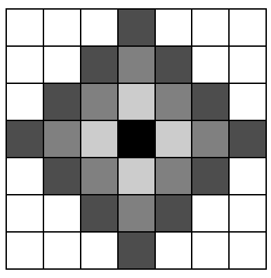
For any \(H \in \mathbb N^+\), we call the \(H\)-neighborhood of a location, the set of locations that are at a Manhattan distance \(H\) of this location. Said differently, for a location at coordinates \((i,j)\), its \(H\)-neighborhood is the set of locations \((i',j')\) such that \( \mid i-i'\mid + \mid j-j'\mid =H\) (not considering the periodic boundary conditions). We illustrate neighborhoods in Figure 1. For all simulations, we use a relevant neighborhood size that we call \(H \geq 1\).
Individuals have a utility to live in a given location, say \(L\). Let \(n_1\) be the number of individuals of type \(1\) in the \(1\)- to \(H\)-neighborhoods of \(L\). Let \(n_2\) be the number of individuals of type \(2\) in the \(1\)- to \(H\)-neighborhoods of \(L\). And finally, let \(n_0\) be the number of empty locations in the \(1\)- to \(H\)-neighborhoods of \(L\). An individual of type \(i\) in location \(L\) has a utility
| $$u^i(n_0,n_1,n_2)=\sum_{k \in \{0,1,2\}} - \left\lvert \frac{n_k}{n_0+n_1+n_2} - t^i_k \right\rvert,$$ |
The dynamics of our model is ruled by the four possible events that occur in continuous time: deaths, births, moves and immigration. We describe these events in the following.
Death. Any individual dies at rate \(\mu\). When an individual dies, the location where it stood before it died becomes of state 0. Notice that we do not consider age categories and that the death rates of natives and immigrants are considered equal.
Birth. Any individual in location \(L\) can give birth to another individual at rate \(\nu\). This birth takes place if there exists at least one empty location in the country. In this case, one of the empty locations is uniformly drawn by chance. We call \(l\) this location. \(l\) changes of state with the following rule.
- If the individual giving birth (in location \(L\)) is of type 1, her child is of type 1 and \(l\) becomes of state 1.
- If the individual giving birth is of type 2, then, her child's type depends on the population in the \(0\) to \(H\) neighborhoods of \(L\). Let \(n_1\) (resp. \(n_2\)) be the number of individuals of type 1 (resp. type 2) in this neighborhood of \(L\)[3]. The probability that the child is of type 1 is a function of the weighted (with weight \(\alpha\)) proportion of \(n_1\) individuals, \(\frac{\alpha.n_1}{\alpha.n_1 + n_2}\). This function is illustrated in Figure 2[5].
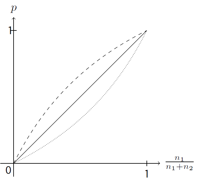
Let us list the implicit assumptions behind our birth dynamics. First, we consider asexual reproduction in order to avoid all matching technicalities. Second, we interpret that when a child comes at the age of living by himself[6], she has to migrate to another country if there is no location left in the country we model. Considering the birth rate as depending on the number of empty locations in the country would be another possibility that would be more artificial in our opinion. Finally, we assume that immigrants' children are raised at their parents' place and, in the neighborhood they live in, they undergo influences that determine their type when grown up and moving away from their parents' place. If raised in a neighborhood with only type 2 individuals, a child becomes of type 2. If raised in an environment with many type 1 individuals, a child likely becomes a type 1 individual. How the proportion of type 1 individuals influences the likelihood of a child to become of type 1 is parametrized by \(\alpha \geq 0\). The larger \(\alpha\), the larger the influence of type 1 individuals on the education of type 2 children in a neighborhood or said differently, the larger the willingness or possibilities to assimilate.
Move. Any individual in location \(L\) has the possibility to move to another location at rate \(m\). This move takes place if there exists at least one empty location in the country. In this case, one empty location is uniformly drawn by chance. We call \(l\) this location. The move to location \(l\) is accepted if the utility that the individual gets from living in \(l\) is strictly larger than the utility that she gets from living in \(L\). This moving process is at the heart of the models inspired by the Schelling model and generates the moving externalities that allows the social outcomes to be often very different from a simple aggregation of individual preferences.
Immigration. At any time, a migration can take place with rate \(e\) under the condition that there exists at least one empty location in the country. Admission of this immigration in the country is made by a democratic process. Each type 1 individual, say in location \(L\), casts her vote depending on the states of the locations in the \(1\) to \(H\) neighborhoods of \(L\). Let \(n_1\) (resp. \(n_2\)) be the number of individuals of type 1 (resp. type 2) in this neighborhood. The considered individual casts a vote \textit{for} immigration if \(n_1+n_2>0\) and \(\frac{n_2}{n_1+n_2}<\frac{t^1_2}{t^1_1+t^1_2}\)[6]. The immigration is accepted if a majority of voters cast a vote for immigration. In this case, one empty location is uniformly drawn by chance and the immigrant, of type 2, settles in this location. We are aware that the voting behavior we chose could certainly be very different. Yet, let us explicit the voting choice model we have in mind. Individuals anticipate that the only way they could be impacted by immigration is if it ever implies a move to their neighborhood (possibly at the arrival of the immigrant). If it is the case, then they would rather have a type 2 individual move close to them rather than a type 1 individual if the ratio of type 2 individuals in their neighborhood is low compared to their optimal such ratio. As for the moving decisions, we do not claim that this is the voting decision that a perfectly rational far-sighted forward looking individual with infinite computational power would make but we assume that this is a reasonable heuristics. Finally, notice that we assume that the rate of immigrants applying to enter the country, \(e\), is constant. Said differently, we implicitly assume that the modeled country is always equally appealing for immigrants and that only the decisions democratically made by natives have an impact on the actual immigration rate.
In Table 1, we display the default parameter values for our simulations. Let us justify the main parameter values for our base case. Life expectancy of individuals is 80 years. We consider that both the native and immigrant populations have fertility rates below replacement level since each individual has had \(\nu/\mu=0.85\) child on average when she dies[8]. The rate to move is such that an individual can move 3-4 times per year if she finds a better place to live. The immigration rate is such that about 0.25% of the population of the country can be welcomed every year if democratically accepted. All individuals have a utility that is maximum when there is no empty location around them and 30% of individuals are of the other type. For any set of parameters considered in this study, results are given for 400 repetitions with initial conditions such that there are 10% of immigrants randomly located on the map and no empty location. In the Appendix, we show an analytical version of our model in order to study how parameters affect the results described in the next Section 3. We also display a robustness analysis (Appendix C).
| Parameter | Unit | Value | Description |
| \(n\) | - | 20 | Grid width and lenght |
| \(\mu\) | year-1 | 1/80 | Individual death rate |
| \(\nu\) | year-1 | 0.85\(\mu\) | Rate for individuals to give birth |
| \(m\) | day-1 | 0.01 | Rate for individuals to give birth |
| \(e\) | day-1 | 0.0025 | Rate to move |
| \(H\) | - | 1 | Neighborhoods size |
| \(\alpha\) | - | 1 | Integration rate |
| \(t^1_0\) | - | 0. | Target in empty location for individuals of type 1 |
| \(t^1_1\) | - | \(1-t^1_2\) | Target in state 1 location for individuals of type 1 |
| \(t^1_2\) | - | 0.3 | Target in state 2 location for individuals of type 1 |
| \(t^2_0\) | - | 0. | Target in empty location for individuals of type 2 |
| \(t^2_1\) | - | 0.3 | Target in state 1 location for individuals of type 2 |
| \(t^2_2\) | - | \(1-t^2_1\) | Target in state 2 location for individuals of type 2 |
Results
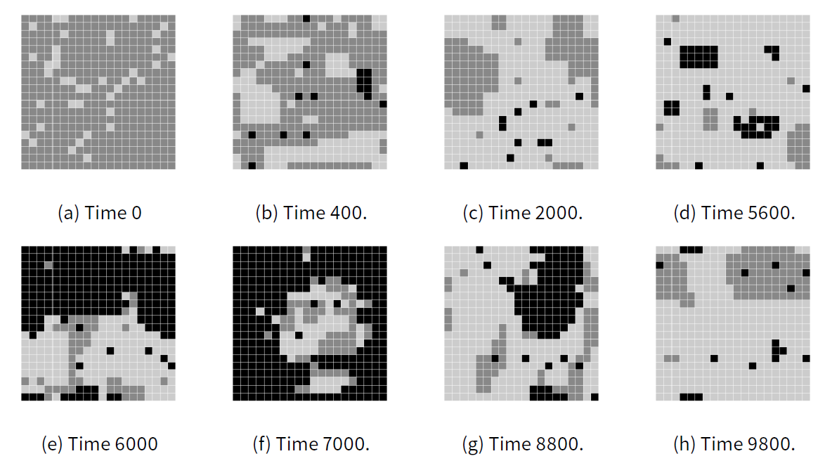
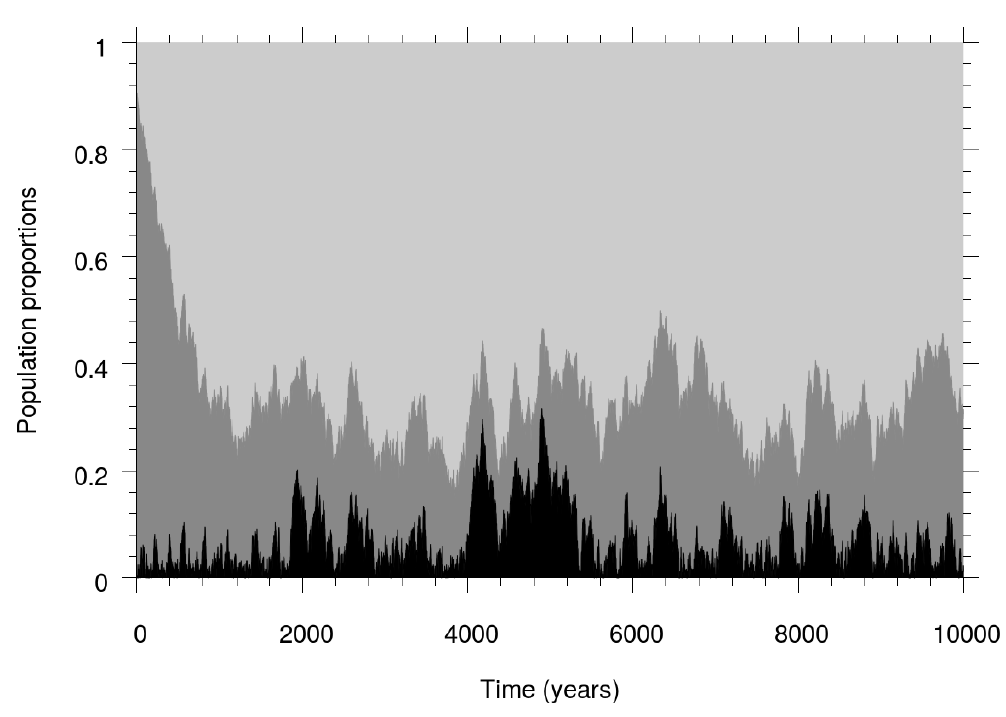
In Figure 3, we display the evolution of the population for one simulation with the base case parameters. In Figure 4, we show the corresponding locations in the country at different dates[9].
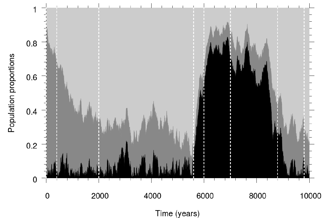
From date 0 to date approximately 400[10], the numbers of births by natives and immigrants are smaller than the number of deaths. As immigrants are not numerous, immigration is political accepted: the number of immigrants increases. After date 400, it continues to increase beyond the 30% mark until date approximately 2,000 when it represents about 70%-80% of the population even though the number of immigrants is much larger than the target of voters which is precisely 30%. This is possible because the possibility for inhabitants to move let them form clusters of individuals of the same type. Notice that the population being clustered is the consequence of the Schelling-like macro-consequence of the unaligned micro-motives for location choices of individuals looking for relatively mixed neighborhoods --~remember that each individuals would be best off with 30% of its neighbors immigrants. In the clusters of natives, only the boundaries vote against immigration whereas cores vote for it. Hence, immigration can be accepted by a large majority of voters who have small numbers of immigrants in their neighborhood even though the ratio of immigrants at the national level is above the natives' target. Between times 2,000 and 5,600, the population is relatively constant with the number of immigrants having assimilated children compensating the death of natives and the death of immigrants being compensated by immigration that is always accepted. We have a reached an equilibrium with a highly clustered population and a very high level of immigrant population very slowly assimilating. However, sometimes, a crisis can occur. This crisis is not necessary[11]. In this instance, at date 5,600, the number of natives becomes too small and immigration is now refused. This implies a decrease of both native and immigrant populations. Then, a situation with a very high level of empty locations is reached. At that date if the relative population of immigrants becomes, again, small enough, immigration is allowed again and we can revert to the first equilibrium. If we define that there is a crisis as the one described above when the number of empty locations is more that 50% of all locations before date 10,000, then 47% (95% CI: 42.2% - 51.9%) of simulations display a crisis. In some instances, this crisis can be so deep that it leads to the disappearance of the native identity. In 1.2% (95% CI: 0.5% - 2.9%) of the simulations, the native identity has totally disappeared from the country before date 10,000. For the rest of the simulations, i.e., conditionally on the native identity not having disappeared before date 10,000, on average, the proportion of empty locations at date 10,000 is 11.1% (95% CI: 9.6% - 12.6%), the proportion of natives is 21.9% (95% CI: 21.2% - 22.5%) and the proportion of immigrants is 67.1% (95% CI: 65.8% - 68.3%).
For the sake of comparison and robustness check, we display in Figure 5, some representative simulations with the same parameter values but for which we don't allow moves or we assume that voting is based on proportions of populations in the entire country, i.e., voting is based on global information and consideration.
Generally, when moves are not allowed and voting is local (one simulation being represented in Figure 5a), at date 10,000, in 14.2% (95% CI: 11.2% – 18.0%) of the simulations the native identity has totally disappeared from the country. For the rest of the simulations, on average, there are 14.6% (95% CI: 12.5% – 16.8%) empty locations, 61.7% (95% CI: 60.1% – 63.3%) natives, 23.7% (95% CI: 23.1% – 24.4%) immigrants. When moves are not allowed and voting is global (one simulation being represented in Figure 5b), at date 10,000, in 8.0% (95% CI: 5.7% – 11.1%) of the simulations the native identity has totally disappeared from the country. For the rest of the simulations, on average, there are 13.2% (95% CI: 11.5% – 14.9%) empty locations, 63.0% (95% CI: 61.7% – 64.3%) natives, 23.8% (95% CI: 23.3% – 24.2%) immigrants. Then, when moves are not allowed, whether voting is global or local has not a large impact on the results and the reason is that when moves are not allowed, populations mix. Hence, the proportions of the different populations in a neighborhood or in the entire country are close. For the same argument, at equilibrium, the voters manage to have the proportion of immigrants close to their optimal level (30% in our case). Also, because the population is well mixed, immigrants’ children assimilate more likely than in the case where moves are allowed and clusters form. This can be seen looking at the next case. When moves are allowed and voting is global (one simulation being represented in Figure 5c), at date 10,000, in 66.2% (95% CI: 61.5% – 70.7%) of the simulations the native identity has totally disappeared from the country. For the rest of the simulations, on average, there are 88.4% (95% CI: 87.0% – 89.8%) empty locations, 7.7% (95% CI: 6.7% – 8.7%) natives, 3.9% (95% CI: 3.4% – 4.3%) immigrants. In this case, voting is global so that for the same reasons as above, the natives vote for a global target of 30% of immigrants. However, now immigrants hardly assimilate. Then, the only way for natives to reach their immigrant target is to refuse immigration. Then, by assumption, the population decreases until the number of natives becomes 0. All results are summed up in Table 2.
| Assumptions | (1) | (2) | (3) | (4) |
| No move allowed, global voting | 8.0% (5.7% - 11.1%) | 13.2% (11.5% - 14.9%) | 63.0% (61.7% - 64.3%) | 23.8% (23.3% - 24.2%) |
| No move allowed, local voting | 14.2% (11.2% - 18.0%) | 14.6% (12.5% - 16.8%) | 61.7% (60.1% - 63.3%) | 23.7% (23.1% - 24.4%) |
| Movers allowed, global voting | 66.2% (61.5% - 70.7%) | 88.4% (87.0% - 89.8%) | 7.7% (6.7% - 8.7%) | 3.9% (3.4% - 4.3%) |
| Movers allowed, local voting | 1.2% (0.5% - 2.9%) | 11.1% (9.6% - 12.6%) | 21.9% (21.2% - 22.5%) | 67.1% (65.8% - 68.3%) |
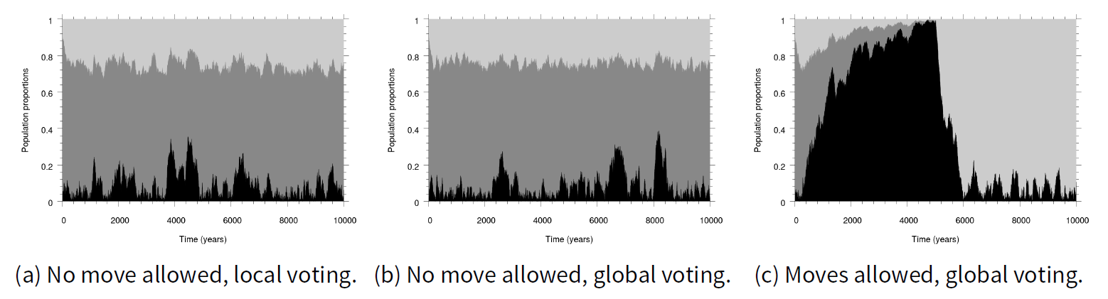
To sum up, if moves are not allowed, whether voting is made on a global or local basis makes only little difference: because populations are mixed, immigrants assimilate, the probability that natives disappear is relatively small and the proportion of immigrants is close to the target ratio. On the contrary if moves are allowed, clusters of individuals with same type form and two cases are possible: either natives' disappearance is close to certain when voting is global or a very large proportion - compared to the optimal proportion of voters - of immigrants is to be accepted when voting is local. In the latter case, the native identity can survive since even a small ratio of the numerous immigrant population assimilating may keep it alive. Also in this case, a very high level of immigrants is democratically imposed by a majority of individuals geographically segregated from immigrants and therefore not in contact with them. This situation of high immigration can be sometimes interrupted by temporary anti-immigration outbursts.
Conclusion
In this article, we study the dynamics of identity and immigration with a model in which political decisions over immigration acceptance are made by a democratic process and living location is endogenous. For the given set of parameter values that we use in the present article, we show the crucial importance of location choices and voting procedure on the long-term future of identity and immigration. When location choices are restrained, the immigrant population is close to what the population with native identity wishes and a stationary state is reached with high assimilation ratio. However, when location choices are implemented, two alternative dynamics can occur. The first possible dynamics, when voting is made on global consideration, leads to a likely disappearance of the native identity. The second possible dynamics, when voting is made on local consideration leads to an unlikely disappearance of the native identity but an immigrant population much more numerous than wished by the population with native identity. The reason for these dynamics is that when individuals are allowed to move, clusters of different types of populations form with the following consequences. First, assimilation becomes more difficult because of the formation of closed communities. Then, when voting is global, the majority voting democratic process leads to the presence of a small immigrant population that is not sufficient to keep the native identity alive through assimilation. Alternatively, when voting is local, the share of population that is not in contact with immigrants forms a popular support for immigration that reaches levels much higher than its optimal one. This numerous immigrant population can keep native identity alive even with low assimilation ratio. In this latter configuration some temporary outbursts of anti-immigration support by the majority can be witnessed.
Let us end this article with an important methodological remark. The present work displays an illustrative model run with parameter values that are not justified very solidly and over time spans that are so long that any reasonable quantitative result can hardly be defended. Our purpose in this article is not to build a model to forecast the long-term future of democracies or to explicit what voters have in mind for the long-term future of democracies. Instead, we believe that the recent electoral successes of the so-called populist movements highlighted the growing concern -at least for western voters- for immigration, the future of identities and assimilation. And our purpose in this article is then to understand at least qualitatively some dynamic mechanisms implied by these legitimate concerns. In particular, we showed the crucial roles of mobility and the level of democracy -local or global- on the common dynamics of immigration and identity. These aspects should therefore be considered in all public debate about these subjects.
Notes
- Notice that an alternative view, the contact theory sees interactions with immigrants typically reducing prejudice, see Allport (1954); Pettigrew & Tropp (2006); Fussell (2014); Paluck et al. (2018).
- Here, in order to be operational, we do not deal with the multiple aspects (Koopmans 2013) or the normative aspects (Kymlicka 1995) of the debate between assimilation vs. multiculturalism.
- We can have an interpretation in terms of any relevant geographical unit, city, region, jurisdiction...
- Notice that since we consider the 0-neighborhood, we have \(L\) included in this neighborhood and hence \(n_2 \geq 1\).
- Notice that \(\frac{\alpha.n_1}{\alpha.n_1 + n_2}=\frac{\alpha\frac{n_1}{n_1 + n_2}}{\alpha\frac{n_1}{n_1 + n_2}+\left(1-\frac{n_1}{n_1 + n_2}\right)}\).
- Without loss of generality, this time is considered the same as biological birth.
- In the following, we will assume that \(t^1_1+t^1_2=1\).
- Notice that without migration, the population of natives would decrease exponentially with a half-life of \(\frac{-\ln(2)}{\nu-\mu}\approx 393\) years. As a consequence, notice that the descendants of the original population will eventually disappear and the native identity can only be kept alive through assimilation.
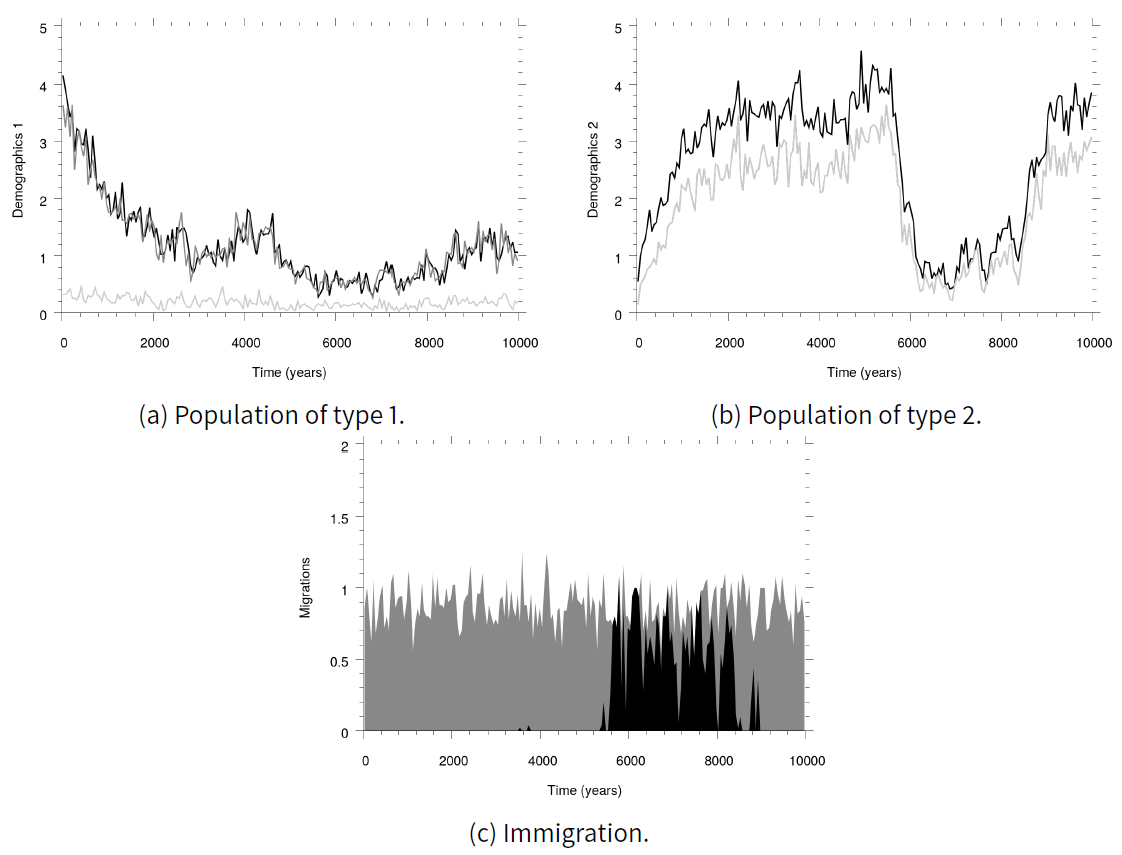
- The corresponding demographic determinants are displayed in Figure 6 in Appendix.
- The dates given here are valid for this simulation. Dates may vary but the global dynamics is often qualitatively unchanged as we will explain later.
- In Figure 7 in Appendix, we show another instance with the population remaining at the same level for more than 10,000 years.
- And we will not defend the rational expectation model stating that both interpretations are necessarily the same.
Appendix
A: More results for the default case
In Figure 6, we show the births and deaths of populations of types 1 and 2 as well as the immigration levels corresponding to simulation displayed in Figure 3 in the main text. In Figure 7, we display another simulation with the same parameter values.
B: Simplified cases taxonomy
Let us start by solving the case with \(alpha=1\), \(H>n/2\) - i.e., the relevant neighborhood is the entire country - and let us assume a continuous country with infinitely many individuals. We will also assume that \(mu > nu\). In this case, our model can be described by the following equations.
| $$\left\{\begin{array}{rcl} \frac{d}{dt}n_{tot}(t)&=&n_{tot}(t)(\nu. \mathbb{1}_{birth}(t)-\mu)+e.\mathbb{1}_{mig}(t)\\ \frac{d}{dt}n_2(t)&=&\left\{ \begin{array}{ll} n_2(t)(\nu\frac{n_2(t)}{n_{tot}(t)} \mathbb{1}_{birth}(t)-\mu)+e.\mathbb{1}_{mig}(t),&\text{ if }n_{tot}(t)>0,\\ e,&\text{ otherwise.} \end{array}\right.\\ \end{array}\right., $$ | (1) |
First, let us see what happens when \(n_{tot}(t)=n_2(t)\). In this case, \(\frac{d}{dt}n_{tot}(t)=\frac{d}{dt}n_2(t)\) and with this constraint, we have one stable stationary point \(n_{tot}(t)=n_2(t)=\frac{e}{\mu-\nu}\) if \(\frac{e}{\mu-\nu}<n^2\). If \(\frac{e}{\mu-\nu} \geq n^2\), the derivative of \(n_{tot}(t)\) is strictly positive \(n_{tot}(t)(\nu-\mu)+e\) everywhere but in \(n_{tot}(t)=n^2\) where it is \(-\mu.n_{tot}(t)\).
In the equation for \(\frac{d}{dt}n_{tot}(t)\), we always have \(n_{tot}(t)(\nu.\mathbb{1}_{birth}(t)-\mu) \leq 0\) when immigration is not allowed and, if immigration is allowed, we have \(\frac{d}{dt}n_{tot}(t)\) has the sign of \(-N+\frac{e}{\mu-\nu}\).
In the equation for \(\frac{d}{dt}n_2(t)\), we always have \(n_2(t)(\nu\frac{n_2(t)}{n_{tot}(t)}-\mu) \leq 0\) when immigration is not allowed and if immigration is allowed, we have \(\frac{d}{dt}n_{tot}(t)\) has the sign of \(frac{\nu.n_2^2}{\mu.n_2-e}-n_{tot}\).
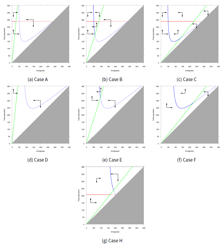
Combining the different cases, we obtain the different possible phase planes displayed in Figure 8 corresponding to parameter values in Table 3. The case we consider in the main text is case E.
Parameter | A | B | C | Case D | E | F | H |
| \(nu\) | 0.85\(\mu\) | 0.85\(\mu\) | 0.85\(\mu\) | 0.85\(\mu\) | 0.85\(\mu\) | 0.85\(\mu\) | 0.3\(\mu\) |
| \(e\) | 0.0015 | 0.0015 | 0.0015 | 0.0025 | 0.0025 | 0.0025 | 0.005 |
| \(t \frac{1}{2}\) = \(t \frac{2}{1}\) | 0.1 | 0.3 | 0.8 | 0.1 | 0.3 | 0.8 | 0.8 |
C: Robustness analysis
In Table 5, we show the alternative parameter values we use for robustness analysis. In Table 6, we display the corresponding outcomes. Notice that in the case in which individuals are not allowed to move, cases Ec and Ed are formally identical to the base case E.
| Parameters’ values | (1) | (2) | (3) | (4) |
| No move allowed, global voting | ||||
| A | 100.0% (99.0% – 100.0%) | 28.5% (27.4% – 29.5%) | 0.0% (0.0% – 0.0%) | 71.5% (70.5% – 72.6%) |
| B | 58.5% (53.6% – 63.2%) | 41.3% (39.0% – 43.6%) | 14.4% (12.3% – 16.6%) | 44.3% (41.4% – 47.2%) |
| C | 0.0% (0.0% – 1.0%) | 28.6% (27.6% – 29.6%) | 53.2% (52.2% – 54.3%) | 18.2% (17.9% – 18.5%) |
| D | 100.0% (99.0% – 100.0%) | 5.5% (5.0% – 6.0%) | 0.0% (0.0% – 0.0%) | 94.5% (94.0% – 95.0%) |
| F | 0.0% (0.0% – 1.0%) | 5.3% (4.8% – 5.8%) | 68.0% (67.5% – 68.5%) | 26.7% (26.3% – 27.0%) |
| H | 100.0% (99.0% – 100.0%) | 48.4% (48.0% – 48.8%) | 0.0% (00.0% – 0.0%) | 51.6% (51.2% – 52.0%) |
| No move allowed, local voting | ||||
| A | 97.2% (95.1% – 98.5%) | 31.1% (29.7% – 32.5%) | 0.3% (0.1% – 0.6%) | 68.6% (67.0% – 70.1%) |
| B | 85.5% (81.7% – 88.6%) | 36.7% (34.7% – 38.8%) | 3.5% (2.3% – 4.6%) | 59.8% (57.4% – 62.3%) |
| C | 0.0% (0.0% – 1.0%) | 27.4% (26.4% – 28.5%) | 54.5% (53.5% – 55.6%) | 18.0% (17.7% – 18.4%) |
| D | 87.2% (83.6% – 90.2%) | 15.4% (13.0% – 17.9%) | 3.1% (2.0% – 4.2%) | 81.5% (78.5% – 84.5%) |
| F | 0.0% (0.0% – 1.0%) | 5.5% (5.0% – 6.0%) | 67.5% (66.9% – 68.0%) | 27.1% (26.7% – 27.4%) |
| H | 100.0% (99.0% – 100.0%) | 48.5% (48.0% – 48.9%) | 0.0% (00.0% – 00.0%) | 51.5% (51.1% – 52.0%) |
| No move allowed, global voting | ||||
| A | 100.0% (99.0% – 100.0%) | 28.8% (27.7% – 29.9%) | 0.0% (0.0% – 0.0%) | 71.2% (70.1% – 72.3%) |
| B | 68.0% (63.3% – 72.4%) | 49.5% (46.6% – 52.4%) | 2.8% (2.3% – 3.4%) | 47.7% (44.5% – 50.9%) |
| C | 0.0% (0.0% – 1.0%) | 27.5% (26.4% – 28.5%) | 59.2% (58.2% – 60.2%) | 13.3% (13.1% – 13.5%) |
| D | 100.0% (99.9% – 100.0%) | 5.0% (4.6% – 5.4%) | 0.0% (0.0% – 0.0%) | 95.0% (94.6% – 95.4%) |
| F | 0.0% (0.0% – 1.0%) | 5.1% (4.6% – 5.5%) | 72.9% (72.4% – 73.3%) | 22.1% (21.8% – 22.3%) |
| H | 100.0% (99.0% – 100.0%) | 48.1% (47.6% – 48.5%) | 0.0% (00.0% – 00.0%) | 51.9% (51.5% – 52.4%) |
| No move allowed, local voting | ||||
| A | 98.5% (96.8% – 99.3%) | 27.5% (26.3% – 28.7%) | 0.0% (-0.0% – 0.1%) | 72.5% (71.3% – 73.7%) |
| B | 3.2% (1.9% – 5.5%) | 36.1% (34.3% – 37.9%) | 24.2% (23.3% – 25.2%) | 39.6% (38.4% – 40.9%) |
| C | 0.0% (0.0% – 1.0%) | 27.6% (26.5% – 28.6%) | 59.1% (58.1% – 60.1%) | 13.3% (13.1% – 13.5%) |
| D | 99.0% (97.5% – 99.6%) | 5.4% (4.9% – 6.0%) | 0.0% (-0.0% – 0.1%) | 94.5% (94.0% – 95.1%) |
| F | 0.0% (0.0% – 1.0%) | 5.0% (4.6% – 5.4%) | 73.2% (72.8% – 73.6%) | 21.8% (21.5% – 22.1%) |
| H | 100.0% (99.0% – 100.0%) | 48.4% (48.0% – 48.8%) | 0.0% (00.0% – 00.0%) | 51.6% (51.2% – 52.0%) |
| Parameter | Case | ||||
| Ea | Eb | Ec | Ed | Ee | |
| \(\alpha\) | 0.5 | 2 | 1 | 1 | 1 |
| \(t^2_1\) | 0.3 | 0.3 | 0.1 | 0.5 | 0.3 |
| \(H\) | 1 | 1 | 1 | 1 | 3 |
| Parameters’ values | (1) | (2) | (3) | (4) |
| No move allowed, global voting | ||||
| E Ea Eb Ee | 8.0% (5.7% – 11.1%) 98.5% (96.8% – 99.3%) 0.0% (0.0% – 1.0%) 0.0% (0.0% – 1.0%) | 13.0% (11.4% – 14.6%) 6.9% (5.7% – 8.0%) 5.9% (5.4% – 6.5%) 5.7% (5.2% – 6.2%) | 58.0% (55.9% – 60.0%) 0.3% (-0.1% – 0.7%) 71.9% (71.4% – 72.4%) 72.0% (71.5% – 72.5%) | 29.0% (27.1% – 30.8%) 92.8% (91.6% – 94.1%) 22.2% (22.0% – 22.4%) 22.3% (22.1% – 22.5%) |
| No move allowed, local voting | ||||
| E Ea Eb Ee | 14.2% (11.2% – 18.0%) 98.2% (96.4% – 99.1%) 0.0% (0.0% – 1.0%) 0.0% (0.0% – 1.0%) | 14.0% (12.0% – 15.9%) 7.5% (6.2% – 8.9%) 5.4% (4.9% – 5.8%) 5.4% (4.9% – 5.8%) | 52.9% (50.3% – 55.4%) 0.0% (0.0% – 0.1%) 72.7% (72.2% – 73.2%) 72.7% (72.2% – 73.2%) | 33.2% (30.8% – 35.6%) 92.4% (91.1% – 93.8%) 21.9% (21.7% – 22.2%) 22.0% (21.7% – 22.2%) |
| Moves allowed, global voting | ||||
| E Ea Eb Ec Ed Ee | 66.2% (61.5% – 70.7%) 98.2% (96.4% – 99.1%) 9.2% (6.8% – 12.5%) 96.5% (94.2% – 97.9%) 14.2% (11.2% – 18.0%) 3.0% (1.7% – 5.2%) | 34.3% (30.5% – 38.2%) 7.0% (5.7% – 8.3%) 63.4% (61.1% – 65.6%) 9.1% (7.4% – 10.9%) 58.1% (55.4% – 60.8%) 68.3% (67.0% – 69.5%) | 2.6% (2.1% – 3.1%) 0.0% (0.0% – 0.1%) 19.9% (18.7% – 21.1%) 0.2% (0.1% – 0.3%) 20.4% (18.9% – 22.0%) 22.0% (21.1% – 22.9%) | 63.1% (58.9% – 67.3%) 93.0% (91.6% – 94.3%) 16.7% (14.4% – 19.0%) 90.7% (88.9% – 92.5%) 21.5% (18.7% – 24.2%) 9.7% (9.3% – 10.1%) |
| Moves allowed, local voting | ||||
| E Ea Eb Ec Ed Ee | 1.2% (0.5% – 2.9%) 75.8% (71.3% – 79.7%) 0.0% (0.0% – 1.0%) 30.2% (26.0% – 34.9%) 0.0% (0.0% – 1.0%) 0.0% (0.0% – 1.0%) | 11.0% (9.5% – 12.5%) 21.6% (18.5% – 24.6%) 5.1% (4.7% – 5.6%) 24.9% (22.2% – 27.6%) 6.0% (5.4% – 6.6%) 7.3% (6.6% – 8.1%) | 21.6% (20.9% – 22.3%) 2.0% (1.6% – 2.4%) 34.5% (33.8% – 35.2%) 8.0% (7.3% – 8.7%) 51.5% (50.9% – 52.1%) 34.8% (34.1% – 35.4%) | 67.4% (66.1% – 68.7%) 76.4% (73.2% – 79.7%) 60.4% (59.7% – 61.0%) 67.1% (64.4% – 69.8%) 42.5% (42.0% – 43.0%) 57.9% (57.3% – 58.5%) |
References
ABBONDANZA, G. & Bailo, F. (2017). The electoral payoff of immigration flows for anti-immigration parties: the case of Italy’s Lega Nord. European Political Science, 17(3), 378–403. [doi:10.1057/s41304-016-0097-0]
ALABRESE, E., Becker, S. O., Fetzer, T. & Novy, D. (2019). Who voted for Brexit? individual and regional data combined. European Journal of Political Economy, 56, 132–150. [doi:10.1016/j.ejpoleco.2018.08.002]
ALLPORT, G. W. (1954). The Nature of Prejudice. Doubleday Anchor.
ARNORSSON, A. & Zoega, G. (2018). On the causes of Brexit. European Journal of Political Economy, 55, 301–323. [doi:10.1016/j.ejpoleco.2018.02.001]
BARONE, G., D’Ignazio, A., de Blasio, G. & Naticchioni, P. (2016). Mr. Rossi, Mr. Hu and politics. The role of immigration in shaping natives’ voting behavior. Journal of Public Economics, 136, 1–13. [doi:10.1016/j.jpubeco.2016.03.002]
BRUNNER, B. & Kuhn, A. (2018). Immigration, cultural distance and natives’ attitudes towards immigrants: Evidence from Swiss voting results. Kyklos, 71(1), 28–58. [doi:10.1111/kykl.12161]
CASELLI, M., Fracasso, A. & Traverso, S. (2018). Globalization and electoral outcomes: Evidence from Italy. SSRN Electronic Journal. [doi:10.2139/ssrn.3194705]
CITRIN, J. & Wright, M. (2009). Defining the circle of we: American identity and immigration policy. In The Forum (Vol. 7, No. 3). De Gruyter. [doi:10.2202/1540-8884.1319]
CLARKE, H. D., Goodwin, M. & Whiteley, P. (2017). Brexit: Why Britain Voted to Leave the European Union. Cambridge, MA: Cambridge University Press. [doi:10.1017/9781316584408]
DANZER, A. M. & Yaman, F. (2013). Do ethnic enclaves impede immigrants’ integration? evidence from a quasi-experimental social-interaction approach. Review of International Economics, 21(2), 311–325. [doi:10.1111/roie.12038]
DAVIS, L. & Deole, S. S. (2015). Immigration, attitudes and the rise of the political right: The role of cultural and economic concerns over immigration. SSRN Electronic Journal. [doi:10.2139/ssrn.2641016]
FLAIG, J. & Houy, N. (2019). Altruism and fairness in Schelling’s segregation model. Physica A: Statistical Mechanics and its Applications, 527, 121298. [doi:10.1016/j.physa.2019.121298]
FUSSELL, E. (2014). Warmth of the welcome: Attitudes toward immigrants and immigration policy in the United States. Annual Review of Sociology, 40(1), 479–498. [doi:10.1146/annurev-soc-071913-043325]
GOODHART, D. (2017). The Road to Somewhere: The Populist Revolt and the Future of Politics. Oxford, UK: Oxford University Press.
GOODWIN, M. & Milazzo, C. (2017). Taking back control? investigating the role of immigration in the 2016 vote for Brexit. The British Journal of Politics and International Relations, 19(3), 450–464. [doi:10.1177/1369148117710799]
HOOGHE, M. & Dassonneville, R. (2018). Explaining the Trump vote: The effect of racist resentment and anti-immigrant sentiments. PS: Political Science & Politics, 51(03), 528–534. [doi:10.1017/s1049096518000367]
INGLEHART, R. & Norris, P. (2016). Trump, Brexit, and the rise of populism: Economic have-nots and cultural backlash. SSRN Electronic Journal. [doi:10.2139/ssrn.2818659]
JENSEN, P., Matreux, T., Cambe, J., Larralde, H. & Bertin, E. (2018). Giant catalytic effect of altruists in Schelling’s segregation model. Physical Review Letters, 120(20), 208301. [doi:10.1103/physrevlett.120.208301]
KAUFMANN, E. (2017a). Can narratives of white identity reduce opposition to immigration and support for hard Brexit? A survey experiment. Political Studies, 67(1), 31–46. [doi:10.1177/0032321717740489]
KAUFMANN, E. (2017b). Levels or changes?: Ethnic context, immigration and the UK independence party vote. Electoral Studies, 48, 57–69. [doi:10.1016/j.electstud.2017.05.002]
KAUFMANN, E. & Harris, G. (2015). ’White flight’ or positive contact? local diversity and attitudes to immigration in Britain. Comparative Political Studies, 48(12), 1563–1590. [doi:10.1177/0010414015581684]
KOOPMANS, R. (2013). Multiculturalism and immigration: A contested field in cross-national comparison. Annual Review of Sociology, 39(1), 147–169. [doi:10.1146/annurev-soc-071312-145630]
KYMLICKA, W. (1995). Multicultural Citizenship: A Liberal Theory of Minority Rights (Oxford Political Theory). New York: Oxford University Press.
LASCH, C. (1996). The Revolt of the Elites and the Betrayal of Democracy. London, UK: WW Norton & Company.
LEE, N., Morris, K. & Kemeny, T. (2018). Immobility and the Brexit vote. Cambridge Journal of Regions, Economy and Society, 11(1), 143–163. [doi:10.1093/cjres/rsx027]
LUBBERS, M. (2008). Regarding the Dutch ’nee’ to the European constitution. European Union Politics, 9(1), 59–86. [doi:10.1177/1465116507085957]
MAJOR, B., Blodorn, A. & Major Blascovich, G. (2016). The threat of increasing diversity: Why many white americans support Trump in the 2016 presidential election. Group Processes & Intergroup Relations, 21(6), 931–940. [doi:10.1177/1368430216677304]
MCLAREN, L. (2012). The cultural divide in Europe: Migration, multiculturalism, and political trust. World Politics, 64(2), 199–241. [doi:10.1017/s0043887112000032]
PALUCK, E. L., Green, S. A. & Green, D. P. (2018). The contact hypothesis re-evaluated. Behavioural Public Policy, 1-30. [doi:10.1017/bpp.2018.25]
PETTIGREW, T. F. & Tropp, L. R. (2006). A meta-analytic test of intergroup contact theory. Journal of Personality and Social Psychology, 90(5), 751–783 [doi:10.1037/0022-3514.90.5.751]
PUTNAM, R. D. (2007). E pluribus unum: Diversity and community in the twenty-first century the 2006 johan skytte prize lecture. Scandinavian Political Studies, 30(2), 137–174. [doi:10.1111/j.1467-9477.2007.00176.x]
SAKODA, J. M. (1971). The checkerboard model of social interaction. The Journal of Mathematical Sociology, 1(1), 119–132
SCHELLING, T. C. (1971). Dynamic models of segregation. The Journal of Mathematical Sociology, 1(2), 143– 186.
SIDES, J., Tesler, M. & Vavreck, L. (2017). How Trump lost and won. Journal of Democracy, 28(2), 34–44. [doi:10.1353/jod.2017.0022]
STEPHAN, W. & Renfro, C. (2002). ‘The role of threat in intergroup relations.’ From prejudice to intergroup emotions: Differentiated reactions to social groups. London: Routledge, pp. 191-207.
SWALES, K. (2016). Understanding the Leave vote. Tech. rep., London: NatCen Social Research: http://natcen.ac.uk/media/1319222/natcen_brexplanations-report-final-web2.pdf.
URSELMANS, L. (2018). A Schelling model with immigration dynamics. In Artificial Life and Intelligent Agents. Cham: Springer, pp. 3–15.
URSELMANS, L. & Phelps, S. (2018). A Schelling model with adaptive tolerance. PLoS ONE, 13(3), e0193950. [doi:10.1371/journal.pone.0193950]