
Introduction
Language scholars speak of language contact to refer to all those situations in which speakers of different languages (or different varieties of the same language) get to interact with one another and, eventually, influence each other’s linguistic behaviour. In particular, Thomason (2001) stresses the interaction aspect. The mere juxtaposition of speakers of different languages is indeed not enough to speak of language contact. Interaction is key for one language group to have an impact on the other, be it exchanging linguistic features across speakers or pushing one group to deviate from its usual speaking behaviour (e.g., switching to another language). Among the numerous social and linguistic implications of language contact, language shift is one of the most commonly observed phenomena. It can be defined as the process whereby, for a number of reasons, a community shifts to speaking a language different from its own. As a matter of fact, close language contact and perceived lower status are often the cause of language decline and, eventually, language extinction. Nelde (2010) rightly observed that language contact is inevitably followed by some form of conflict, which often comes to the detriment of some less powerful, possibly minority language community. The idea of conflict should not be strictly interpreted as a violent clash between groups. Rather, it should be interpreted as a form of competition over limited resources, such as funds devoted to media in one or another language or time spent speaking one language or another.
Hornberger (2010) defines language shift as the gradual displacement of one language by another in the lives of the community members. He notes that factors contributing to it are complex and diverse. They have been observed to be of political, social, economic, cultural, and, clearly, linguistic nature (Conklin & Lourie 1983). Over time, governments have implemented numerous policy interventions concerning language decline. Often, the cause of failure has been the presence of non-linguistic variables which were not addressed by policy intervention and eventually played a crucial role in the decline process.
Language contact is a recurring phenomenon in population dynamics and its implications for regional and minority languages represent a complex issue. As I shall argue in the rest of this paper, the implications of language contact depend on many variables simultaneously at play. The direct consequence of this is that traditional approaches to language issues, which are often studied from one disciplinary perspective at a time, often fail to detect all the factors at play in language dynamics. Surprisingly, the acknowledgement that language issues have implications in social, political and economic terms did not automatically lead to an interdisciplinary approach. In the past few years, many scholars have come to the conclusion that language issues are complex and call for an interdisciplinary approach in order to look at all dimensions simultaneously[1]. Language dynamics are ultimately linked to the complexity of individual language behaviours and their continuous interplay, which develops into collective behaviours and eventually decides the fate and fortunes of every language. Collective behaviours are often hard to predict and disentangle and thought experiments often represent an important tool, in that they go beyond classical observation methods and switch the focus from correlation to causation (Gabbriellini 2018). Nevertheless, thought experiments may be hard to perform, especially when they concern phenomena that involve somewhat unintuitive or unexpected dynamics. In this context, computer simulations allow to systematically explore the implications of intuition and can make us aware of unpredictable patterns that we would otherwise overlook. This paper develops an agent-based model (ABM) that describes language dynamics as the result of complex interactions. ABMs simulate all sorts of dynamics based on the interactions of individuals acting within a system in which new variables can be added, subtracted and modified to project different scenarios[2]. These variables do not only represent standard information such as the number of individuals and their linguistic endowments and skills, but also situational conditions, such as social relations, people’s attitude towards socio-cultural differences, their propensity to pick up a new language, government intervention in the education system, and so on. Besides, ABM programming tools allow for the calibration of such variables, which respond to – and with – different levels of intensity. As a consequence, ABMs can not only help sketch the current situation and its future dynamics, but also provide an idea of the consequences to which different policy interventions might lead. Indeed, ABMs are most typically developed to either increase our understanding of the mechanics of real-world systems, or predict how changes in different factors can affect the dynamics of the real-world systems (Williams 2018).
The rest of this paper is structured as follows. First, I introduce the notion of language contact by briefly reviewing the relevant literature and discussing the various aspects of language contact that allow us to consider it a complex issue in the formal sense of the term (Section 2). Second, I briefly introduce agent-based modelling and explain why it is useful in the study of population dynamics (Section 3). Third, I present a model of language contact developed in the NetLogo programming environment (Wilensky & Rand 2015) and its underlying hypotheses (Section 4). Finally, I discuss the simulations performed, the statistical methods used to analyse the data and the results of the analyses (Section 5 and Section 6). The main contributions of this paper are, first, to show that macro-level language contact dynamics can be explained by relatively simple micro-level behavioural patterns and, second, to provide further support to qualitative discussions already presented in previous studies. The resulting model can then be used to make projections of short- and long-term trends of language decline and to estimate the relative impact of a number of different factors, including those that are “policy-actionable,” i.e. that can be addressed through policy.
Language Contact and Bilingualism
A simple yet effective definition of language contact is provided by Thomason:
"[L]anguage contact is the use of more than one language in the same place at the same time. (Thomason 2001, p. 1)."
This definition effectively highlights a first fundamental element of language contact, i.e. coexistence. For language contact to happen, two languages need to “exist'' concurrently. However, Thomason herself immediately points out two problems with such a trivial definition. The first issue is that two (groups of) speakers of different languages in the same place at the same time may ignore each other. In that case, no transfer of linguistic features would occur and we could only speak of language contact in its purely literal sense. Therefore, coexistence is a necessary but not sufficient condition. Indeed, interaction is a second crucial condition for language contact to have sociolinguistic consequences. The second issue is that this definition does not clarify what is meant by “language''. One might simply assume that language contact occurs when speakers of different codified languages interact with one another, which would be far from incorrect. However, linguists tend to speak of language contact in a broader sense to include also interactions between speakers of different variants of the same language. Different syntax patterns, deviations from some specific pronunciation, the use of slang and local terms can all cause individuals to have trouble understanding one another, even if they are indeed speaking the same language. Besides, I shall point out that the expression “in the same place” should not be interpreted too strictly, especially at a time when information technology allows communication to happen smoothly over long distances. Thomason (2001) does not provide a strict spatial definition. Indeed, language contact can happen at different level on a spectrum that stretches from micro (e.g., two individuals speaking different languages working in the same office) to macro (e.g., along the language border within a bilingual country).
Appel & Muysken (2005) note that some form of bilingualism is a common consequence of language contact. They speak of two types of bilingualism, individual and societal, to distinguish between bilingualism as the individual ability of speaking two languages from bilingualism as a feature of a society where two languages are spoken. Furthermore, they identify three types of societal bilingualism, generally described as follows[3]:
- two languages are spoken by two different groups and each group is monolingual, typical, for example, of early colonial settlements, where the colonizer and the colonized would each speak his or her own language;
- two languages are spoken and everybody is bilingual, a situation often found in many African countries, where individuals often have command of the language of the former colonizer in addition to one or more local languages;
- two languages are spoken, but one group is monolingual and the other is bilingual. An example of this type might be Ireland, where virtually everyone has full command of English and some are also able to speak Irish, though at different levels of fluency. A similar example is to be found in Friesland, a region in the North of the Netherlands, with Dutch and West Frisian.
Interestingly, Switzerland provides examples of each of the mentioned typologies (all of which, however, need to be taken with a pinch of salt, in that the categorization of multilingual communities is rarely as clear-cut as presented above):
- First, the country has four national languages, and for three of them (German, French and Italian) it is possible to identify areas with relatively clear-cut borders. Although language regions have no legal recognition whatsoever, keeping in mind that cantons have sovereignty on all matters except those that are shared with or delegated up to the Federal government, linguistic communities are fairly independent from one another. Indeed, out of 26 cantons, only three are officially bilingual (French-German) and one officially trilingual (German-Italian-Romansh). As a matter of fact, it is rather common for Swiss people to live most of their life on their side of the linguistic border and only use their language for most of their time.
- Second, in German-speaking cantons, standard German (Hochdeutsch) is the official language[4], but many German-speaking Swiss, though proficient in standard German, would consider their local Swiss German dialect (e.g. Baseldytsch, Bärndütsch or Züridütsch, respectively the dialects of Basel, Berne and Zurich) to be their native language[5].
- Third, the Swiss canton of Grisons is the only one where Romansh is an official language, along with German and Italian. Being a very small minority that has been shrinking over the last century, virtually all Romansh-speakers have full command of another Swiss language, most of the time (Swiss) German, since childhood. Clearly, the reverse does not apply to German-speaking and Italian-speaking residents of Grisons, who are only seldom fluent in Romansh.
Each of these cases would call for an ad hoc study, and therefore I needed to make a choice. Throughout the rest of this article I will concentrate on the third typology of societal bilingualism.
Speaking of bilingualism, there is no overall agreement of whether a bilingual individual should be one who has native-like command of both of her languages, or simply anyone who has some knowledge of a second language, or anything in between[6]. For the purposes of this article, I will call “bilingual” any individual who alternatively uses two languages based on the situation, regardless of her level of fluency. As said, it is assumed that all minority-language speakers are fluent in the majority language. It follows that any minority language speaker qualifies as a bilingual in our simulated environment, even if they have very limited knowledge of the minority language.
Some authors (for example, Sperlich & Uriarte 2014; Grin 2016) have noted the competitive nature of language choice for plurilingual individuals and compared the dynamics surrounding language use to market-like dynamics of scarce resource allocation. Indeed, individuals need to allocate a limited amount of resources (in particular, time) over the languages they speak, whether it means having a conversation or reading a book in one language or another. Clearly, every individual tries to allocate her resources in order to maximize her utility (defined here as a measurement of the satisfaction that an individual gains from an activity that can be performed in different languages). However, the allocation process does not operate independently of certain constraints. For example:
- the use of a specific (probably majority) language might be expected or even mandatory at work or in education, implying that during certain hours, individuals are not free to choose what language to use;
- leisure opportunities in the minority language(s) might be few compared to those in the majority language and/or more costly, due for example to a limited availability of translated books or dubbed films;
- the utility provided by activities in the minority language (just as in any language) is highly dependent on the level of fluency of individual speakers. Indeed, supposedly pleasant activities, such as conversing or reading a book in a minority language, might as well result in a feeling of frustration if they are not backed by sufficient fluency.
Uriarte (2016) defines language contact as the most extreme form of language competition, whose pressure is particularly felt by the minority language community. Indeed, we can identify several factors that will influence (if not effectively shape) the linguistic behaviour of minority-language speakers. In a seminal paper, Giles et al. (1977) discuss the idea of “language vitality” and classify the factors affecting it in three categories:
- status factors, which include variables such as the socio-economic conditions of speakers, the perception of the language in terms of prestige (or lack thereof), and the socio-historical weight of the language;
- demographic factors, which include variables such as the absolute number of speakers and rates of emigration and immigration;
- institutional support factors, which include the formal and informal support to the language provided by various institutions, such as legal recognition and language education programs.
As I discuss in Section 4, the model of language contact presented in this article takes into consideration variables from all of these categories. From the first category, I will consider the likelihood for minority-language speakers to reveal their cultural background, which is clearly influenced by how the language is perceived by society. For example, if a certain minority language is generally linked to backwardness or lower social classes, people may prefer not to be associated with it. Therefore, they might hide their cultural background from their interlocutor if they are not certain that they are speaking to another minority language speaker. Conversely, if a language is perceived as having a certain prestige, minority-language speakers might be happy or even proud to show it by addressing people directly in the minority language[7].
Concerning the second category, the model includes variables such as the initial total population, the proportion of minority-language speakers, population growth rates and life expectancy. Finally, concerning the third category, the model allows for the implementation of language education programs specifically addressed to minority-language speakers with a view to boosting their skills in the minority language. I shall also point out that, although I do draw on the typology of factors proposed by Giles et al. (1977), I will not strictly abide by their view on them. Their discussion on the implications of these factors and the causation links between them and language vitality have been discussed and by and large criticized by Grin (1990, 1992). In particular, Grin suggests that a higher level of language vitality is not necessarily related to a higher likelihood of survival. As we will see, this paper partly confirms the idea that language decline might happen regardless of its initial level of vitality (see Section 5).
Agent-Based Modelling and Population Dynamics
Agent-based modelling has been an important methodology in the study of population dynamics and, in the past decade, it has known renewed fame as a consequence of the massive progress in information technology and computational power. Generally speaking, researchers use agent-based modelling to describe population dynamics by relying on theories from other disciplines and translating them into behavioural rules to apply in the context of computer-based models. Van Bavel & Grow (2017) note that population studies have always been characterized by a “closed” approach where populations are treated as entities with their own macro properties. In this top-down approach, inter- and intra-population dynamics are mainly described through indicators. The “closed” approach has proved very successful and laid much of the theoretical groundwork of the discipline. However, Kreager (2015) points out that this approach comes at the expense of a more “open” approach that would prioritize the study of the processes and networks arising from the interactions among heterogeneous agents and their environment. The focus of such an approach would be on the study of the mechanisms behind patterns of association among individuals. However, such an open approach inevitably calls for a reorientation of the research paradigm from an exclusively macro-level perspective to one that also looks at the micro level. More precisely, it requires the analysis to take on a perspective that stretches along a micro-to-macro spectrum. Indeed, macro-level dynamics are inevitably the result of interactions among micro-level agents. Nevertheless, many of these dynamics cannot always be inferred directly by looking only at what happens at the micro level. In complex phenomena such as population dynamics, it is unsurprisingly the case that the macro level displays properties which are more than the simple sum of its micro-level components.
Agent-based modelling provides the right amount of flexibility to handle such complexity, as it allows for an effective representation of the feedback cycle between the micro and the macro level. Referring to Hedström & Swedberg (1998), Van Bavel & Grow (2017) explain the link between the micro and the macro level by means of a three-step macro-micro-macro model, widely known as “Coleman’s boat” (Coleman 1990). The first step describes the situational mechanisms, that is, how the characteristics of the macro level shape the context in which individuals interact. The second step looks at the action formation mechanisms, i.e. the individual interactions at the micro level and how they are affected by the situational mechanisms defined at the macro level. Finally, in the third step the analysis moves on to study the transformational mechanisms, i.e. the way in which individual actions and interactions affect the macro context and bring about social change. It is exactly this third step that Billari (2015) considers the most interesting and challenging for scholars in the field of demography. The macro-micro-macro model can be graphically represented as shown in Figure 1 (adapted from Van Bavel & Grow 2017).
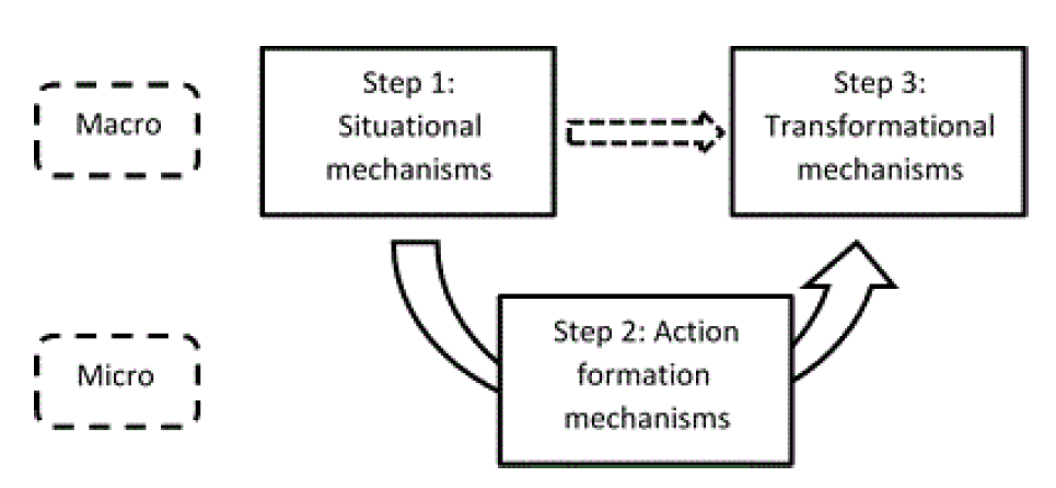
This three-step visualization can be easily adapted to the structure of the model presented in this article. First, we look at the macro-level elements embodied in the model, including not only demographic conditions such as total population and growth rate, but also the linguistic landscape, i.e. the fact that two languages are spoken according to a certain distribution. Second, we give agents behavioural rules to manage language use, given the macro-level conditions. Third, we look at how their behaviour affects the macro-level context, in particular the language distribution.
One of the reasons why many scholars advocate the use of computational models in the study of population dynamics is that they lend themselves particularly well to sensitivity analysis, with which we can evaluate the relative impact of different parameters on the output of the model (Grow 2017). In particular, the model presented here can be used mainly in two ways:
- to make projections starting from existing conditions;
- to estimate the potential impact of policies addressing one or more of the factors included in the model.
Before I move on to present the details of the ABM presented in this paper, I will discuss in short some notable examples of modelling language contact and explain in brief how the model that I present in this paper differs from them.
Modelling language contact
The tradition of modelling language contact is not recent. Indeed, the literature on this topic is rich and wide. An in-depth discussion of this literature is well beyond the scope of this paper, but a short review seems due in order to provide the reader with a bird's eye view on the topic. In particular, many models of language competition take on a differential equation approach. Simply put, these models try to develop a mathematical formulation that is able to describe observed trends in language growth or decline (i.e. the rates of change, whence the use of differential equations). One notable example of such approach is provided by Abrams & Strogatz (2003). They describe the case of a community where two monolingual groups co-exist and develop a concise yet effective model that describes the rate of change of speakers of languages X and Y in terms of the probabilities of switching from one language to the other. These probabilities are in their turn dependent on the relative amount of speakers and the perceived status of each language. The authors go on to show how their formulation fits well historical data from several instances, such as the case of Scottish, Quechua and Welsh. Isern & Fort (2014) build on the model by Abrams & Strogatz and add a spatial dimension to it. By adapting the reaction-diffusion model, most commonly used for modelling the change of concentration and spread of chemicals, they estimate the speed at which a language spread over a geographical area replacing the local language.
Minett & Wang (2008) are among the first to move the focus from differential equations to agent-based modelling, recognizing that differential equation models work well in so far as individual behaviour can be neglected so that one can focus on aggregate trends. The authors explore the effect of language status and education policies on the maintenance of a minority language. Another related example of modelling language contact is provided by Castelló et al. (2013), who also take on an agent-based modelling approach. Starting from the acknowledgement that language contact is a complex phenomenon, they develop and ABM that explores the dynamics of a community where two languages are spoken, each with a share of monolingual and bilingual speakers. They pay particular attention to how language status and individual likelihood to shift to another language impact language growth and decline. However, the main focus of their study is on the spatial dimension of social networks, i.e. they explore the impact of different types of spatial configuration on language dynamics (in terms, for example, of language segregation). Networks are an important element in the study of language contact, as noted by Milroy (1980). Therefore, Castelló et al. (2013) provide one of the first attempts to combine a quantitative approach with a sociolinguistic perspective.
Another interesting example is provided by Patriarca et al. (2012), who, on top of providing a very interesting review of different methodologies used in the study language contact, also discuss the possibility of adopting a game-theoretical approach. For this purpose, they discuss two different strategies encountered among minority-language speakers, i.e. addressing people in the minority language or not. As I will discuss later, this kind of reasoning also serves as basis for one of the behavioural rules of the agents in the ABM presented here. The authors acknowledge that, regardless of the methodology adopted, a clear understanding of the mechanisms underlying language contact is still missing and that more empirical work is needed to inform modelling. They suggest that future research should focus, among other things, on the impact of variables such as language prestige and language policies on patterns of local interactions. The model that I present here follows by and large this rationale. In this article, I try to bridge the gap between the purely economic thinking and the sociolinguistic perspective. Abrams & Strogatz (2003), as well as most of the mathematical models that build on theirs, refer to on a non-better defined “transition rate,” which, in turns, depends on a variable taking on values between 0 and 1 that should reflect the advantages that the languages gets from a higher status. This latter variable is, in my opinion, somewhat obscure, possibly as a consequence of a relative disregard of the sociolinguistic literature. It is indeed not the status that eventually decides the fate of a language, but rather how this status translates into practice. For example, a language might be official, and therefore enjoy “high status.” Yet, if people do not have a desire, an opportunity or simply the capacity to speak it, a high status will not save it from extinction (Grin 2003). By treating status as a single variable, a model can provide valuable insights, yet it remains obscure as to what exactly affects the vitality of a language. By combining the economic and the sociolinguistic approach, I try to break down the status variable into a more “operationable,” more transparent set of variables. This line of reasoning is not new in the literature of language contact. For example, this is also the view of Zhang & Gong (2013). They argue that the variables usually found in the mathematical models of language competition are too abstract and that such studies should focus on more concrete parameters. It is not unexpected that such observations come from two authors that are well versed in the language sciences.
An ABM of Language Contact
Before presenting the details of the model, I will discuss its underlying assumptions. The model assumes that the two communities differ only in the languages they speak, one being able to speak only the majority language and the other being able to speak both the majority and the minority language. As discussed previously, a community in which two languages are spoken can be, generally speaking, either a community with an ethnolinguistic minority within it (such as the Arbëreshë, speakers of a variant of Albanian living in some villages of Southern Italy, or Romansh-speakers in German-speaking Switzerland) or an ethnically homogeneous community where only some individuals are able to speak a certain language (for example, Irish speakers in Ireland). In particular, I assume that minority language individuals are perfectly integrated and that it is not possible to single them out on the basis of a peculiar accent or some physical traits. Besides, an important implicit assumption made by the model is that minority-language speakers are willing to bear a certain level of frustration in order to speak (and therefore support the maintenance of) the minority language.
We conceptualize the utility of conversing with another individual as depending on two variables: the level of proficiency of the interlocutors and the preference for one specific language. Concerning the first variable, it is reasonable to assume that more proficient speakers will be able to discuss a broader range of topics with no difficulty. As I said, every individual in the environment is fully proficient in the majority language. Therefore, if we conceived utility only as a function of proficiency, following the principle of least effort in efficient communication (Zipf 1949), we would conclude that minority-language speakers:
- are indifferent between speaking the majority or the minority language, if both interlocutors are fully fluent in both languages;
- prefer to communicate in the majority language (in which they are assumed to be fully fluent), if at least one of the interlocutors has less-than-full knowledge of the minority language.
Formally, we could write
| $$u(A) \geqslant u(B)$$ | (1) |
However, as said, we conceptualize utility as being also a function of the specific language used to communicate. minority-language speakers of our virtual community will always be willing to speak the minority language when presented with the opportunity, regardless of their level of fluency. Therefore, we are implicitly assuming that there exists an additional utility stemming from the mere fact of speaking the minority language. This additional utility is always more than enough to compensate the fact that minority-language speakers are not always able to hold a fully satisfying conversation in it. Formally, it reverses the inequality as follows:
| $$u(A) < u(B)$$ | (2) |
This additional benefit can be seen as a non-linguistic consequence most likely related to the emotional attachment of minority-language speakers to their language. Indeed, it is reasonable to assume that minority-language speakers are happy to have an opportunity to speak and, therefore, support their language. Obviously, this greater utility is only accessible if both interlocutors speak the minority language. If one of the interlocutor is a monolingual majority language speaker, the minority language speaker is forced to choose the majority language.
Model specifications
The model has the following characteristics:
- The environment in which the agents live, though visually represented as a square by the NetLogo interface, has a toroidal topology, i.e. all of the edges are connected to another edge in a doughnut-like shape. Therefore, agents are free to move in any direction at any time. The choice for an open environment over a closed one is made to avoid that agents get stuck in corners or against the edges, which could distort the results.
- The environment is a multilingual community in which two languages are spoken, majority language A and minority language B. The initial proportion of individuals of either community can be determined before launching the simulation. The two languages are assumed to be linguistically distant, so that mutual intelligibility is excluded and mixed conversations (i.e. happening partly in language A and partly in language B) are not possible. Besides, it is assumed that there are no migration flows.
- For the reasons discussed in Section 2, every individual is assumed to be fully fluent in the majority language and some individuals are also able to speak the minority language with varying degrees of fluency. Following Grin et al. (2010), the initial distribution of fluency among speakers of the minority language follows a doubly-truncated normal distribution, with lower and upper limits of 1 (almost no useful knowledge of the language) and 100 (full proficiency), around a mean that can be determined through the model interface before launching the simulation.
- Depending on their personality type, some minority-language speakers are always willing to start the conversation in the minority language (reveal type), while others will prefer to speak the majority language and switch to the minority language in case they find out that their interlocutor is also a minority language speaker (hide type). The ratio of reveal-to-hide individuals can be determined before launching the simulation. The rationale underlying such distinction is further explored in Section 4.9 and following.
- Every time-step represents one year.
- The population grows at a certain rate which can be calibrated and differentiated between the two communities. Women aged between 14 and 50 are “fertile” and, based on a fertility rate, might give birth to a child. By analogy with communication behaviour rules, minority children born to families where both parents speak the minority language also speak the minority language and inherit the level of fluency of their mother. As we assumed that communication between minority-language speakers and majority-language speakers can only happen in the majority language, babies born to mixed couples are assumed to be majority individuals with no fluency in the minority language[8]. This (admittedly strong) assumption is a simplification largely based on Solèr (2004), who discusses in depth different linguistic behaviours in various family scenarios and goes on to distinguish many more cases. Besides, Lüdi et al. (1997), speaking of the case of Switzerland, note that German tends to impose itself as the only communication language in German-Romansh families even in areas with a high presence of Romansh-speakers[9].
- The likelihood of exogamous pairing can be determined before launching the simulation by the exogamy rate variable.
- Individuals die when they reach a certain age, which can be manually set. All other causes of death are not taken into consideration, in that we have no reason to believe that the incidence of fatal events is different between the two communities.
- The government can decide to put in place special education plans specifically intended for minority-language speakers aged between 6 and 18 in order to boost their language skills (during these years, their fluency increases by ten units at every time-step). The policy can either be in place at all times or activated only if the proportion of minority-language speakers falls below a certain threshold. Besides, it can be addressed to all minority-language speakers or only a part of them. By the end of the program, students are assumed to have reached full proficiency, regardless of their initial level.
Model specifications are an intentionally simplified version of real-life dynamics. Indeed, one of the objectives of this article is to show that it is possible to propose an explanation of complex macro-level patterns by tracing them back to relatively simple micro behavioural rules. Support for this claim is provided by validating our ABM through real-world data (see Section 4.20 and following).
Before moving on, I will spend a few words on the communication dynamics within mixed households, whose impact on the minority language is captured by the exogamy rate variable. One could argue that this assumption does not seem to be reasonable, in that it is not unusual to observe bilingual households. However, relaxing this assumption would mean splitting the exogamy rate variable in two, one variable defining the likelihood that a female minority-language speakers picks a majority language partner and the other defining the likelihood that the minority language is passed on to the offspring of such mixed couple. Exogamy rate is conceptualized as the probability with which minority language women have a child from a majority language man. However, in practical terms (i.e. in the source code) it is the probability with which the offspring of a minority language woman is not a minority-language speakers (e.g., if exogamy rate is 30%, then there is 30% chance that the offspring born to a minority language woman is a majority-llanguage speakers only, as, implicitly, the baby is born to a majority language father). However, this can also be interpreted to mean that, even in mixed households, the minority language is passed on with a certain probability (for example, if exogamy rate is 0%, it could mean that, even in mixed households, the minority language is always passed on to the next generation). Obviously, this could be treated differently. We could split this in two parts. First, modelling the actual probability of minority women to choose and majority partner, and then adding an extra parameter to model the probability with which the child born to a minority mother and a majority father acquires the minority language. However, having two nested distributions vary simultaneously would not provide more insights than having one distribution (as defined above) vary, as long as its meaning is clearly laid out. The reason why I decided to code it this way is because I wanted to keep a direct relationship between the impact of each parameter and potential policy measures. In other words, I tried to model directly the net impact of the two variables. I tried to define the parameters in a “policy-actionable” way, so that, once we have defined their impact, we can evaluate the extent that our potential policy intervention should have. Indeed, as I argue at the end of the paper, one cannot really influence (democratically, that is) people’s choice of a partner to have a child, but one can influence the communication behaviour in their household. Influencing the attitude of mixed households would in fact amount to influencing the exogamy rate variable defined the way I do.
Types of minority-language speakers
As Uriarte (2016) points out, communication can be thought of as a so-called cheap talk game, originally introduced by Crawford & Sobel (1982). Cheap talks are opposed to signalling processes, in that in the latter sending messages may be costly for the sender and can happen in several possible ways, while in the former it is free and happens mainly through ordinary talk. Crawford & Sobel (1982) describe the following setting:
- there are two players, a sender (\(S\)) and a receiver (\(R\));
- \(S\) has some information about a certain state of the world, \(\theta\), described by a value over a closed interval \([0,1]\), which is unknown to \(R\);
- \(S\) can decide to send a message to \(R\) at no cost, which can correspond exactly to \(\theta\) or deviate from it by a parameter \(b\);
- based on the information received, \(R\) takes action \(y\) (also described by a real number) that maximizes her utility \((u_{R})\).
The payoffs of the two players are described by the following quadratic utility functions (Ganguly & Ray 2012):
| $$u_S (y,\theta,b)=-(y-(\theta+b))^2$$ | (3) |
| $$u_R (y,\theta)=-(y-\theta)^2$$ | (4) |
The sender \(S\) conveys the amount of information that causes the receiver \(R\) to react in a way that maximizes the sender’s utility (\(u_S\)). The parameter \(b\) represents the divergence of interests between the two players, or bias. The receiver wants to take the action that matches the state of the world in order to maximize \(u_R\). Indeed, we can take the partial derivative of \(u_R\) with respect to \(y\), the only parameter that \(R\) can control, and get
| $$\frac{\partial u_R}{\partial y}=2\theta-2y$$ | (5) |
To find the maximum of the function, it is enough to set this derivative equal to zero and check that the second derivative is negative. It follows that \(u_R\) is maximized for \(y=\theta\), as the second derivative is negative (and equal to -2). This can be easily seen in Figure 2.

Conversely, the sender maximizes her utility \(u_S\) by choosing how much information to reveal in order to get the receiver to take an action that matches the state of the world plus a certain deviation. Indeed, \(S\) can control parameter \(b\), and if we differentiate \(u_S\) with respect to it, we get
| $$\frac{\partial u_S}{\partial b}=2y-(2b+2\theta)$$ | (6) |
Therefore, \(u_S\) is maximized for \(y=\theta+b\). We could assume that there is no conflict of interests between two players who speak the minority language, in that, as explained above, I assumed that every minority language speaker is willing to speak the minority language whenever presented with the opportunity. Therefore, we have a case in which \(b=0\) and both utilities are maximized when the sender fully discloses the state of the world (i.e., reveal that she speaks the minority language by addressing her interlocutor in it) and the receiver reacts accordingly (by replying in the minority language). We could conclude that minority-language speakers have an interest to always speak the minority language as a first choice. Nevertheless, minority-language speakers might also meet a monolingual speaker, who, by definition, is only able to speak the majority language. According to linguistic politeness theory (Brown & Levinson 1987), individuals will choose a communication strategy that minimizes confrontation. Indeed, addressing someone directly in the minority language might be perceived as a face-threatening act, in that the interlocutor might be forced to reveal her lack of knowledge of the minority language. As a consequence, the sender wants to avoid this kind of situation. In other words, her utility would be reduced if it turned out that the interlocutor did not speak the minority language, as she would feel that she has been "impolite" by addressing the non-minority interlocutor in the minority language. This matter is largely cultural and can vary greatly across different societies. For example, the seriousness of face-threatening acts depends largely on the level of power distance that exists in a given society, defined as “the extent to which the less powerful members of organizations and institutions accept and expect that power is distributed unequally” (Hofstede 2011, p. 9). Indeed, they are perceived as much more serious in societies characterized by higher levels of power distance, such as Asian and African countries, than it is in societies where it is less pronounced, such as Northern European countries. Note that this behaviour could also be seen as a specific form of communication accommodation. We speak of communication accommodation when people make behavioural changes in their communication strategy to converge or diverge from their partner. For example, accommodation can be used to reduce the perceived socio-cultural distance between two individuals by making one's speech pattern more similar to one's interlocutor. Conversely, one might stress some aspects of one's own way of speaking to highlight the very same differences. In the case of the model presented here, the decision by a minority language speaker of not addressing her interlocutor directly in the minority language can be seen as a form of linguistic convergence to reduce distance[10].
To strike a balance between the economic reasoning presented above and the considerations on linguistic accommodation, we distinguish between two categories:
- those for whom the reduction in utility stemming from being “impolite” is greater than the extra utility deriving from speaking the minority language – these individuals will not address people in the minority language, unless they are sure that their interlocutor also speaks the minority language;
- those whose extra utility more than compensates the potential reduction – these individuals will always try to speak the minority language.
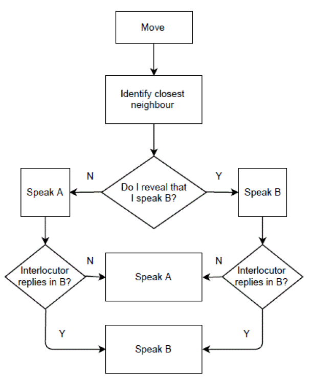
Therefore, following Sperlich & Uriarte (2014), we distinguish between these two types of minority-language speakers according to their personality. Speakers of the minority language can be willing either to reveal their linguistic background or to hide it. Uriarte (2016) defines them as individuals who are, respectively, strongly loyal or weakly loyal to the minority language. In the model presented here, a reveal-personality individual will always start the conversation in the minority language and only switch to the majority language if her interlocutor cannot speak the minority language. Conversely, a hide-personality individual will always start the conversation in the majority language and will only reveal her background if another minority language speaker addresses her in the minority language. The background of the person starting the conversation is not important, in that it is assumed that a reveal-personality minority speaker will reply in the minority language even if she is addressed in the majority language and then switch to the majority language if it turns out that her interlocutor speaks only the majority language. Intuitively, a graphic representation of this process could be as presented in Figure 3. Obviously, the communication behaviour of (monolingual) majority-llanguage speakers is much less articulated, in that they will always speak language A.
Interactions
Starting from the age of 6, every individual explores the environment and interacts with her closest individual at every time-step. Every time-step can be seen as one year. Interactions happen based on the following rules:
- if two majority-llanguage speakers meet, they will converse in language A and nothing happens in relation to language B;
- if a minority language speaker meets a majority language speaker, they will converse in language A and the proficiency in language B of the former will be slightly reduced;
- if two language B speakers meet, the way they interact depends on their personalities:
- if two hide-personality individuals meet, they will not know that they are both able to speak the minority language and they will converse in the majority language, causing their level of fluency in the minority language to be reduced;
- if at least one reveal-personality person is involved, the conversation will be held in the minority language and the level of fluency increases for both.
At every time-step (i.e. at every iteration of the model), every minority language individual locates her closest agent and, based on whether the closest agent is a minority language speaker or not, adjusts her level of knowledge of the minority language, respectively positively or negatively by one unit. This is a mechanic way of conceptualizing the fact that interacting in the minority language will increase one's fluency in it, while not doing it does the opposite. At every time-step, if there are \(n\) minority-language speakers, there are going to be \(n\) such interactions (majority-llanguage speakers are always assumed to speak the majority language, so nothing happens to their fluency). Obviously, in real life it is not one single conversation that makes a significant difference in one's level of fluency. For this reason, I try to capture in one interaction the effect of a long series of conversations, which is why I characterize one time-step as one year. For a minority language speaker, one interaction with a majority- (minority-)language speaker can be seen as a year in which one used the majority (minority) language more often than the other. Indeed, there would be no practical gain in breaking down this effect in hundreds and hundreds of micro-interactions, which would each have a micro-impact on the level of fluency and which, summed up, would give a net negative or positive overall impact. Simple as they are, these interactions capture the idea that, throughout a year, minority-language speakers might have more or less frequent opportunities to use the minority language, which will eventually affect their level of fluency. If their level of fluency reaches zero, they are assumed to be completely assimilated in the majority community and are considered simple majority-llanguage speakers from then on.
In the following sections I will first validate the model and then I will discuss the results of a number of simulations. I will concentrate on the likelihood of survival of the minority language as a consequence of variables such as the proportion of minority people having a reveal-personality, education policies and the threshold at which they are put in place. I will also spend a few words on the impact of these variables on the level of fluency of minority-language speakers.
Model validation
Before discussing the results of the simulations, the model needs to be validated by comparing its results with real wold data, in order to make sure that the assumptions on which it is based and the trends that it estimates are in a sense illustrative of reality. In the domain of computer simulations, a model that is a good representation of the real system is said to have face validity (Carson 2002). It could be easily argued that, given the need for simplifications, models are unrealistic anyway. However, agent-based modelling, just as any type of modelling, should be seen as an instrument to gain insights into a phenomenon and not as a truthful representation of reality. Even if based on drastic simplifications of reality, models can help gain better understanding of a phenomenon, which can in turn help our intuition to explain it or make predictions about it. As the objective of this article is to provide an idea of the relative impact of the variables taken into consideration on the decline of minority languages, it is not crucial that numbers are exactly right. Nevertheless, a close approximation of observed data is still desirable.
As discussed in Section 2, Switzerland provides various examples of language competition. In particular, I will compare the model presented here with the situation of Romansh-speakers in the trilingual canton of Grisons. As mentioned, Grisons is Switzerland’s largest canton in terms of surface, the only trilingual one and the only one where Romansh is an official language[11].
As they constitute a shrinking minority, virtually all Romansh speakers (with the possibly sole exception of very young children) are proficient in the majority language of the canton, i.e. German (along with the local Swiss German dialect) (Liver 1999; Solèr 2004). According to the Swiss Federal Statistical Office, only 0.5% of the resident population of Switzerland declares Romansh as a main language (De Flaugergues 2016). The Romansh language has an important cultural and identity value for Romansh people. According to Solèr (2004), in areas where Romansh is spoken, it is very common for Romansh-speakers to meet allophones, mostly German speakers, and Romansh is only used with other Romansh-speakers. In this regard, he notes that Romansh-speakers often face a dilemma, in that (i) being upfront about their background and constantly choosing to address people in Romansh without knowing if they speak the language is often considered rude, and (ii) constantly giving up Romansh in favour of German to accommodate allophones may be perceived by others as an act of betrayal towards not only one’s own native language, but also one’s own cultural heritage. The Romansh-speaking and the German-speaking communities live together with a high level of integration in virtually all areas where Romansh is spoken. Solèr (2015) notes how there exists virtually no Romansh-only area and this has been especially the case since 2010, when many officially Romansh-monolingual municipalities started being merged with other German-monolingual municipalities to create larger bilingual administrative units. Besides, mixed pairs made up of a Romansh speaker and a German speaker are also a common feature of Romansh-language communities (Osswald 1988). Considering all of the above, it is possible to conclude that Romansh-speaking areas in the canton of Grisons are by and large well represented by the simulated environment of the model and can be used as a source for validation.
The next step in our validation process is to check whether the trends estimated by the model are comparable to the trends actually observed. In order to do this, the model needs to be calibrated so as to reflect actual contextual data of the region taken into consideration. As a consequence, historical data from the canton of Grisons have been averaged over the period considered for validation, i.e. from 1960 to 2000, and used to calibrate the model before launching the simulations. Then, I have compared the results generated by the simulations in terms of the decline in the relative number of Romansh-speakers with the actual trends observed over the same period. In order to account for the intrinsic stochasticity of agent-based models, I have run 100 simulations with the same initial conditions and averaged the results.
Some data were not directly available and needed to be estimated. Taking into consideration only Romansh-speakers and German-speakers (excluding italophones and other allophones), the former represented 31.52% of the combined Romansh- and German-speaking population of Grisons in 1960, while the latter represented 68.48%[12]. According to the World Bank[13], the average fertility rate in the canton of Grisons between 1960 and 2000 was 1.81 (child per 100 women per year), which I assumed to be the same for both language communities. Average life expectancy, which rose from slightly more than 71 in 1960 to almost 80 in 2000, was 75.4. According to Osswald (1988), in 1960, couples involving at least one Romansh speaker involved another Romansh speaker in 60.75% of the cases and an allophone in the rest of the cases. This value had decreased linearly to 57.47% in 1970 and 52.14% in 1980. However, these values consider all possible combinations, including Italian speakers and other allophones. These data are complemented, and partly contradicted, by the data provided by the Swiss Federal Statistical Office, which allow to distinguish different types of combinations. If we consider only households where Romansh and/or German are spoken, regardless of whether a third language is also spoken, we obtain estimates that vary roughly between 60% and 65% between 1970 and 2000. Therefore, I combined the two sets of data and considered an average rate of endogamous pairing of roughly 60% between 1960 and 2000. The proportion of reveal-to-hide personality individuals is hard to estimate, therefore I simply assumed that the two personality types are equally represented in the community, as everybody faces the dilemma explained earlier. Concerning education policies in support of the Romansh language, we kept them inactive for these simulations in that the use of Romansh in schools was significantly increased only in 1990, at the end of our simulated period, when, on average, roughly 54.5% of students living in the traditional Romansh-speaking areas used Romansh as a communication language (Lüdi et al. 1997, p. 269). However, the use of Romansh in education varies significantly across the different Romansh-speaking communities. In 1990, the use of Romansh in school varied from less than 10% of the students in the Sutsilvan area to almost 90% in the Vallader area (Furer 2005).
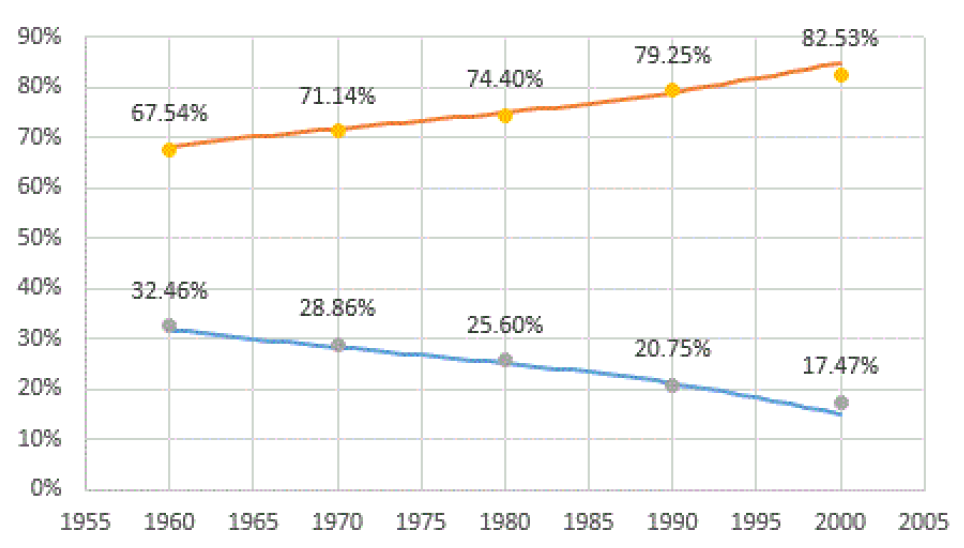
Figure 4 shows the average of the simulated trends of Romansh speakers (blue curve) and German-speakers (orange curve) proportions between 1960 and 2000 based on the conditions explained above. The trends are compared to the proportions actually observed (yellow and grey dots). The estimates were adapted from Coray (2008), taking into consideration only Romansh and German speakers. Surveys for the period 1960-1980 asked people about their “mother tongue”, while those for the years 1990 and 2000 allowed respondents to distinguish between “main language” and “language of common use”[14].
As the latter option is much less restrictive than the former, for sake of consistency, I decided to stick to the estimates of speakers of Romansh as main language, which was defined in the survey as the language of which respondents have the best command. Therefore, I consider “main language” more akin to the idea of “mother tongue” than “language of common use”. The model seems to project actual trends quite well. Therefore, we can consider the analysis of the results produced by the model as reasonably reliable, even if it is based on relatively simple behaviour rules.
Data Generation and Analysis
In this section, I first discuss how I used the model to perform simulations and generate data, then I review the statistical methods used to analyse the data and produce results. I concentrate on the impact of different variables on the trends of the proportion of minority-language speakers. I also briefly discuss the impact of the same variables on the level of fluency of minority-language speakers. However, as statistics on people’s language skills are harder to obtain and less reliable as often based on self-assessment, the model was only validated for the proportion of minority-language speakers. Consequently, results concerning the level of fluency should be taken with a pinch of salt. Nevertheless, I considered it useful to add them to the discussion of the model, in that they can still provide some interesting insights. Finally, I will briefly present some results concerning the relationship between vitality and long-term survival of minority languages.
The specifications used in the simulations performed for the first analysis are summarized in Table 1. The first five parameters are necessary because they provide the model with dynamics, but I set them on arbitrary values because I am not interested in their impact. The last four are allowed to vary and were combined to create different scenarios to simulate.
| Parameter | Value (range) | Meaning |
| Initial population | 200 | Agents at the beginning of the simulation |
| Initial proportion of minority speakers | 40% | Proportion of the population able to speak the minority language |
| Growth rate of the majority community | 2% | - |
| Growth rate of the minority community | 2% | - |
| Life expectancy | 80 | - |
| Exogamy rate | 0% to 100% (in steps of 10%) | The likelihood with which a female minority individual gives birth to a baby with a majority individual |
| Reveal strategy | 0% to 100% (in steps of 10%) | The proportion of minority-language speakers that are willing to reveal that they speak the minority language |
| Education | 0% to 100% (in steps of 10%) | The proportion of minority-language speakers in school age that receive education in the minority language, if a language education plan is in place |
| Minority threshold | 0% to 50% (in steps of 10%) | The threshold under which the proportion of minority has to fall before a language education plan is put into place[15] |
Each combination of variables was simulated ten times to account for variations due to the intrinsic stochasticity of ABMs. A time limit of 1,000 time-steps was set. The number of scenarios simulated was 7,986, while the total number of simulations was 79,860.
The first analysis puts the decline of minority-language speakers in relation with the variables mentioned above. It is divided in two parts. First, I run a linear regression using the number of steps until extinction of the minority language community (i.e. until the proportion of minority-language speakers to total population reaches zero) as a dependent variable and the variables mentioned above as independent variables. Second, I run a logistic regression to estimate the probability of surviving in the long term depending on the same independent variables as for the first part.
For the first part, I only look at the sub-sample of populations where the minority community disappeared within 1000 steps, which corresponds to roughly 95% of the total sample. Therefore, the new sample consisted of 75,541 observations. A quick look at the data shows a few issues that need to be taken into account before moving on to the analysis. By taking a look at the average number of steps-to-extinction per level of each variable, we immediately notice that the impact of all variables, especially the rate of exogamy, is non-linear. I shall note in passing that non-linearity is a common feature of complex systems. To account for this curvature, I will do two things. First, as it is common in these cases, I centre the predictors about their mean values and include the square of each predictors. Centring data is done to avoid that the linear and the quadratic term correlate with one another. Second, I take the logarithm of the number of steps and use it as a dependent variable. This is a common transformation used to linearize non-linear relations. Besides, this helps hedge another issue, i.e. heteroscedastic data. However, to account for any heteroscedasticity left in data, we shall still use robust standard errors to compute more reliable test statistics and their related p-values. The resulting regression equation is the following:
| $$\begin{split} ln(y)=\beta_0+\beta_1 exogamy.rate+\beta_2 reveal.strategy+\beta_3 education+\beta_4 minority.threshold\\ +\beta_{11} exogamy.rate^2+\beta_{22} reveal.strategy^2+\beta_{33} education^2+\beta_{44} minority.threshold^2+\epsilon \end{split}$$ | (7) |
The results of the regression analysis are reported in Table 2.
| Estimate | Std. Error | t-value | Pr(>|t|) | Sig. | |
| (Intercept) | 5.584000 | 0.002355 | 2370.99 | <2e-16 | *** |
| Exogamy rate | -0.018260 | 0.000032 | -569.94 | <2e-16 | *** |
| Reveal strategy | 0.001711 | 0.000030 | 56.79 | <2e-16 | *** |
| Education | 0.002651 | 0.000030 | 87.81 | <2e-16 | *** |
| Minority threshold | 0.005303 | 0.000056 | 95.08 | <2e-16 | *** |
| (Exogamy rate)2 | -0.000065 | 0.000001 | -56.84 | <2e-16 | *** |
| (Reveal strategy)2 | -0.000043 | 0.000001 | -40.24 | <2e-16 | *** |
| (Education)2 | -0.000052 | 0.000001 | -47.77 | <2e-16 | *** |
| (Minority threshold)2 | -0.000260 | 0.000004 | -68.04 | <2e-16 | *** |
The (adjusted) \(R^2\) of the model is 0.829, meaning that the regressors can explain almost 83% of the variance in the dependent variable, while the remaining 17% can be traced back to the intrinsic stochasticity of complex systems. Bearing in mind that the high number of predictors included in the model tend to inflate the value of the \(R^2\), we can say that the model is a good fit for the data. All of the predictors are statistically significant. However, given the great amount of data, statistical significance was almost expected and is not really informative. Interpreting the estimated coefficients when quadratic terms are included is somewhat less intuitive than it is for usual regression with linear predictors only. Indeed, each linear predictor needs to be interpreted together with its corresponding quadratic term. Besides, for the sake of easier interpretation, we need to retransform the coefficients to account for the fact that we used the logarithm of time-steps as a dependent variable. The impact of the independent variable \(x\) on the predicted value \(y\) is the change in the predicted value when \(x\) changes by some amount \(\delta x\), ceteris paribus, i.e. when all other variables are held constant. We start by looking at the fitted model (for sake of simplicity, I will stick to the case of one linear predictor and its corresponding quadratic term):
| $$ln(\hat{y}(x))=\hat{\beta}_0+\hat{\beta}_1x+\hat{\beta}_{11}x^2$$ | (8) |
| $$ln(\hat{y}(x+\delta x))-ln(\hat{y}(x))=\hat{\beta}_0+\hat{\beta}_1(x+\delta x)+\hat{\beta}_{11}(x+\delta x)^2-\hat{\beta}_0-\hat{\beta}_1x-\hat{\beta}_{11}x^2$$ | (9) |
| $$ln\bigg(\frac{\hat{y}(x+\delta x)}{\hat{y}(x)}\bigg)=\hat{\beta}_1\delta x+\hat{\beta}_{11}(2x\delta x+(\delta x)^2)$$ | (10) |
Note that this last passage is the same regardless of the number of predictors included in the model. As they are kept constant in order to compute the impact of the variable \(x\) only, they cancel out, as was the case for \(\hat{\beta}_0\). Provided that the change in \(x\) is small and that size of \(\hat{\beta}_{11}(\delta x)^{2}\) is insignificant compared to the remaining terms on the right-hand side (that is, when \(|\hat{\beta}_{11}\delta x| \ll |\hat{\beta}_1+ 2\hat{\beta}_{11}x|\)), we can rewrite the equation above as
| $$ln\bigg(\frac{\hat{y}(x+\delta x)}{\hat{y}(x)}\bigg)\approx (\hat{\beta}_1+ 2\hat{\beta}_{11}x)\delta x$$ | (11) |
The left-hand side is the logarithm of the relative change in the predicted response \(\hat{y}(x)\). On the right is a multiple of the (small) change \(\delta x\) in the regressor. The relative change in \(\hat{y}\) is going to be
| $$\frac{\hat{y}(x+\delta x)}{\hat{y}(x)}\approx \exp((\hat{\beta}_1+ 2\hat{\beta}_{11}x)\delta x)$$ | (12) |
As can be seen, the relative change depends on the value of \(x\) with which one starts. In other words, the change in the response is not constant and depends on the value of the regressor. Therefore, contrary to linear-linear regression, the estimated coefficients in log-linear regression do not represent the slope of the curve. Finally, we can observe that, for small values of \(\delta x\), the right-hand side of the previous equation can be rewritten as
| $$\exp((\hat{\beta}_1+ 2\hat{\beta}_{11}x)\delta x)\approx 1+(\hat{\beta}_1+ 2\hat{\beta}_{11}x)\delta x$$ | (13) |
| $$\frac{\hat{y}(x+\delta x)}{\hat{y}(x)}\approx 1+(\hat{\beta}_1+ 2\hat{\beta}_{11}x)\delta x$$ | (14) |
| $$\hat{y}(x+\delta x)\approx \hat{y}(x)(1+(\hat{\beta}_1+ 2\hat{\beta}_{11}x)\delta x)$$ | (15) |
This means that that the ratio between successive fitted values of \(y\) is linear in \(x\) or, alternatively, that the new value \(\hat{y}(x+\delta x)\) is approximately equal to the previous value \(\hat{y}(x)\) times a change of \(100%*(\hat{\beta}_1+ 2\hat{\beta}_{11}x)\delta x\). This linear approximation helps us interpret the results of the regression analysis in a more intuitive way. If we consider positive unitary changes (i.e., \(\delta x = 1\)), we can find, for example, the range of variation in the impact of each variable from their minimum to maximum value[16],reported in the last column of Table 3.
| Impact of linear predictor | Impact of quadratic predictor | Range of relative change | |
| Exogamy rate | -1.826% | -0.007% | 98.82% - 97.54% |
| Reveal strategy | 0.171% | -0.004% | 100.60% - 99.75% |
| Education | 0.265% | -0.005% | 100.79% - 99.76% |
| Minority threshold | 0.530% | -0.026% | 101.83% - 99.28% |
Table 3 is interpreted as follows. The first two columns are simply the beta coefficients in percentage terms, the same reported in Table 2. The last column indicates the ratio between successive fitted values of \(y\). Values above 100% means that successive values increase, while values below 100% indicate a negative succession. Values very close to 100% imply that successive values are very close to one another or virtually unchanged. Exogamy rate seems to be by far the strongest predictor. Consecutive fitted values of \(y\) are initially about slightly less than 99% of the preceding value when \(x\) increases by one unit. As \(x\) increases, this decrease tends to accelerate (as it could be guessed from the fact that the coefficients of the linear and quadratic terms are both negative). Indeed, when \(x\) is high, a unitary increase causes successive values to be between 98% and 97.5% of their preceding values. All other predictors have a positive but relatively weak impact on the long term survival of the minority community. Among them, minority threshold seems to be the strongest. Therefore, teaching the minority language to minority individuals to make them fluent seems to have a positive impact, especially if we consider that the variable education also has a positive coefficient. When the minority threshold is low (i.e. when the proportion of the minority community has to be very small before education plans are put in place), each unitary increase causes successive values of \(y\) (time-steps to extinction) to be almost 102% of the preceding value. However, as suggested by the negative coefficient of the quadratic term, this effect tends to wane as the threshold increases. Successive values tend to be very close to one another, as indicated by a relative change very close to 100%. The same applies to the other two predictors.
For sake of completeness, I also show a graphic representation of the impact of each predictor.
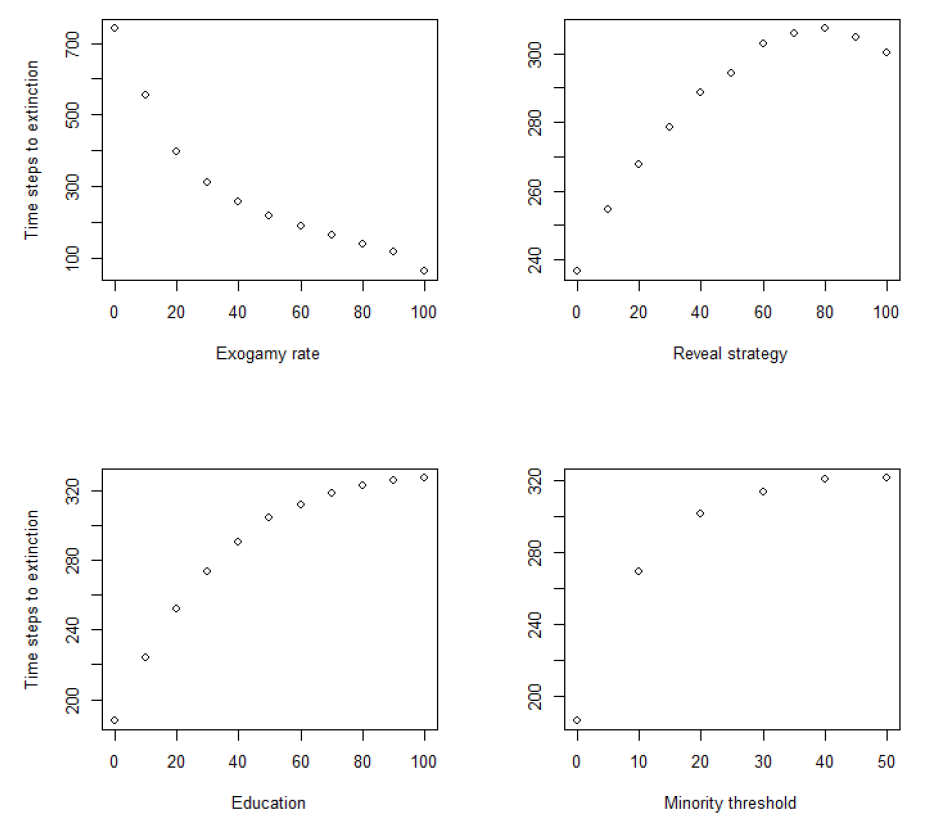
The graphs in Figure 5 plot the average number of time-steps until extinction of the minority community for each separate variables. The other variables also vary, but the contribution of one variable at a time is displayed. As can be seen, each variable contributes to the variation in time to extinction of the minority community. The plots also confirm the sign and the intensity of each variable (note the different scale for the exogamy variable), exogamy being clearly the strongest, and the other predictors having a smaller, yet non-negligible, effect. Besides, the curvatures of these trends justify the choice to add quadratic terms to the regression equation.
The second part of the first analysis consists in using logistic regression to provide further confirmation to the estimated impact of the variables mentioned above on the likelihood of long-term survival of the minority language community. In this part, I use the same database generated for the first part, but I will not exclude those simulations where the minority community went extinct within 1,000 time-steps. Indeed, we are interested in comparing simulations where the minority community survived with those where it did not. As mentioned, the minority language community survived in only 5% of the simulations. To increase the proportion of surviving communities for comparison purposes, I looked at those communities that were still alive after 500 time-steps. The proportion of simulations in which the minority community survived beyond 500 was about 14% of the total. Therefore, the question that we are trying to answer here is: “How are the odds of surviving beyond 500 time-steps affected by our predictors?”
The logistic regression model looks as follows:
| $$ln\bigg(\frac{p(y)}{1-p(y)}\bigg)=\beta_0+\beta_1 exogamy.rate+\beta_2 reveal.strategy+\beta_3 education+\beta_4 minority.threshold$$ | (16) |
As can be seen, this is again a linear model. However, the predictors are in a linear relationship with the logarithm of the odds of a certain event (in our case, the minority language community surviving beyond 500 time-steps)[17].
From the equation above, we can compute the odds as follows:
| $$\frac{p(y)}{1-p(y)}=\exp(\beta_0+\beta_1 exogamy.rate+\beta_2 reveal.strategy+\beta_3 education+\beta_4 minority.threshold)$$ | (17) |
The advantage of reporting the odds rather than the probability is that the variation in the odds is constant for all values of the predictors. It only depends on the magnitude of the variation. Indeed, assuming the case of two independent variables \(x_1\) and \(x_2\) and a variation \(\Delta k\) in \(x_1\), we can compute the odds ratio:
| $$\frac{\frac{p(y|x_1=k+\Delta k)}{1-p(y|x_1=k+\Delta k)}}{\frac{p(y|x_1=k)}{1-p(y|x_1=k)}}=\frac{exp(\beta_0+\beta_1(k+\Delta k)+\beta_2x_2)}{exp(\beta_0+\beta_1k+\beta_2x_2)}=exp(\beta_1\Delta k)$$ | (18) |
Therefore, if we assume unitary increases, the variation in the odds is constant and equal to \(e^{\beta_1}\).
Although it is customary to assign a value of 0 to a negative event (or an event that did not happen) and a value of 1 to a positive event (or an event that did happen), I preferred to assign 0 to the cases in which the minority language community “died” within 500 time-steps and 1 to those where the community did not die, regardless of the final proportion with respect to the majority language community[18]. This does not imply any technical difference in the procedure of coefficient estimation. However, this way the signs of the estimated coefficients are consistent with the results of the previous analysis and easier to interpret. The results of the logistic regression are reported in Table 4.
| Estimate | Exp(coef) | Exp(coef)-1 | Std. Error | z-value | Pr(>|z|) | Sig. | |
| (Intercept) | -3.09506 | 0.04527222 | -0.9547278 | 0.062164 | -49.79 | <2e-16 | *** |
| Exogamy rate | -0.20383 | 0.81560056 | -0.1843994 | 0.002298 | -88.72 | <2e-16 | *** |
| Reveal strategy | 0.017651 | 1.01780779 | 0.01780779 | 0.000595 | 29.66 | <2e-16 | *** |
| Education | 0.04314 | 1.04408437 | 0.04408437 | 0.000708 | 60.95 | <2e-16 | *** |
| Minority threshold | 0.077953 | 1.08107185 | 0.08107185 | 0.001299 | 60.02 | <2e-16 | *** |
The results of the logistic regression analysis seem to confirm the finding of the previous analysis. We can concentrate on column two (“Exp(coef)”) and three (“Exp(coef)-1”). Predictors with negative values in the third column can be seen as “risk” factors, while those with positive values can be seen as “protective” factors. Exogamy rate is once again the strongest predictor. A unitary increase in the rate of exogamy multiplies the odds of surviving beyond 500 time-steps by a factor of about 0.82, or, equivalently, causes a variation in the odds of about -0.18. The second strongest predictor is, once again, minority threshold, followed by education and reveal strategy. While the latter predictor has only a slight impact on the odds of survival, the combined effect of the two education-related variables is substantial. A unitary increase in both variables multiplies the odds of surviving beyond 500 time-steps by a factor of about 1.13[19].
Let us explore further the weight of the exogamy rate variables. Figure 6 shows a heat map plotting the proportion of minority-language speakers to the total populations at time-steps 0 through 500 (recorded every 50 time-steps) for exogamy rates 0% through 50%. The initial proportion of minority-language speakers for these simulations was 40%. Reveal-strategy was arbitrarily set at 60%, minority-threshold at 100%, and education at 20%. This corresponds to a fictitious scenario in which 1 in 5 students is involved in education plans (which are always active, regardless of the proportion of minority-language speakers) and a bit more than 1 in 2 minority-language speakers is willing to converse in the minority language from the onset. These values were kept at constant values as having them vary and then averaging them over all simulations would have confounded the effect of the variables under study and made the heat maps all but non-informative.
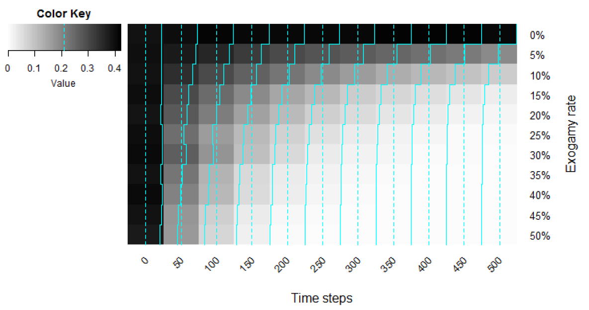
The blue lines at every timestep represent the proportion of the minority community for the exogamy rates indicated. Obviously, at time 0, it’s almost a line, in that they all start at 0.40 (the little wiggles are due to the in-built stochasticity of NetLogo). As we move from left to write we observe two things. First, shades go from darker (more minority speakers) to lighter (less minority speakers) at increasing speeds for increasing exogamy rates. Second, the line is less and less regular: it stays high at 0% exogamy rate, but it becomes lower and lower over time and it does so at increasing speed for higher exogamy rates.
Figure 7 shows a heat map exploring the interaction between reveal strategy and education to see to what extent education needs to be supported by an inclination to speak the minority language. In these simulations I assumed that exogamy rate is 0%, which, as I explained above, can be interpreted to mean either that there are no mixed households or that the minority language is always passed on to the next generation in mixed households. Besides, minority-threshold was again at 100%, so that the education variable is always active. As above, these variables were kept constant.
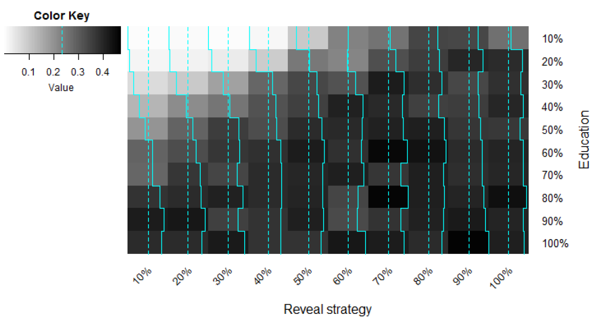
Darker shades represent higher proportion of the minority language community after 500 time-steps. The heat map shows that education policy is effective only if it is backed up by a willingness of the people to speak the minority language as first choice strategy. Indeed, a good deal of the upper-left corner of the map has clearly lighter shades of grey, indicating that even having education policies that involve 50% of the minority language community can have disappointing results if less than 40% of minority-language speakers are hide-type individuals.
In the second analysis I used linear regression analysis to study the factors affecting the impact of the same variables on their fluency of minority-language speakers in the medium term. Therefore, a time limit of 100 steps was set. However, as said, I will not spend too much time discussing these results, in that the ABM was only validated for the proportion of minority speakers, as accurate statistics on people’s language skills are hard to obtain and less reliable as often based on self-assessment. The model has the mean level of fluency of minority-language speakers as a dependent variable. The independent variables are the same as above, i.e. minority-threshold, exogamy-rate, reveal-strategy, and education. This time, all of them were allowed to vary between 0% and 100% in steps of 10%. Each scenario was simulated five times. The number of scenarios simulated was 14,641, while the total number of simulations was 73,205. Of all these simulations, I only included in the analysis those that did not result in complete assimilation within 100 time-steps, which were 65,985, i.e. roughly 90.1%. Obviously, if the minority community is completely absorbed into the majority, the level of fluency is zero. The direct consequence of this choice is that the coefficient of the exogamy rate variable might be underestimated, in that, as we have seen, it has the strongest impact on the survival of minority language communities. Therefore, the observations excluded are more often those with very high level of exogamy. Nevertheless, as the objective of this second analysis is to provide an estimate of the relative impact of all variables in minority language communities that still exist in the medium term, I found it appropriate to exclude cases of full assimilations. Results are reported in Table 5. All regressors in Table 5 have a statistically significant impact on the level of fluency of minority-language speakers. As was the case for the previous analysis, the extremely low p-values are most probably a consequence of the very high amount of data. Clearly, they all have a positive impact, except for exogamy rate. Unlike the previous analysis, the relative impact does not vary substantially across regressors, and education seems to have the biggest effect. The model has an (adjusted) \(R^2\) of 0.618, meaning that almost 62% of variation in the response variable is explained by the regressors, while the rest is due to stochasticity.
| Estimate | Std. Error | t value | Pr(>|t|) | Sig. | |
| (Intercept) | 32.803818 | 0.155221 | 211.3 | <2e-16 | *** |
| Exogamy rate | -0.253376 | 0.001644 | -154.1 | <2e-16 | *** |
| Reveal strategy | 0.236482 | 0.001484 | 159.4 | <2e-16 | *** |
| Education | 0.298659 | 0.001484 | 201.3 | <2e-16 | *** |
| Minority threshold | 0.195549 | 0.001484 | 131.8 | <2e-16 | *** |
I conclude by quickly presenting some results concerning the relationship between vitality and long-term survival of minority languages. The third analysis puts in relation the initial proportion of bilingual speakers (varying between 10% and 90% in steps of 5%) with the number of time-steps until language disappearance. All other variables were kept constant at some arbitrary values. There were 17 different scenarios, and each one was run 20 times, making a total of 340 simulations. Giles et al. (1977) suggest that language vitality feeds on itself. In other words, more used languages tend to have higher chances to survive in the long term. Grin (1992), through formal economic modelling, argues that this is not necessarily the case, i.e. vitality is not always associated with higher survival likelihood. As noted by Grin (1992), the view on vitality and long-term survival provided by Giles et al. (1972) is somewhat circular, in that survival is simultaneously described as an indicator of vitality and a consequence thereof. Therefore, it is not really possible to conclude that vitality feeds on itself. The computational simulation presented here contributes to the qualitative discussion of Giles et al. (1977) and the economic modelling of Grin (1992). My analysis seems to support the idea that language vitality per se can hardly be considered a major driver of minority language survival. Indeed, the results suggest that there is only a weak positive correlation between the initial proportion of bilingual speakers and time to extinction. Besides, this correlation tends to wither and almost disappear for initial proportions higher than 40% (this trend is graphically presented in Figure 8). In other words, a small group of minority-language speakers can survive for a very long time, while a high initial proportion is in no way guarantee of long-term survival. This allows us to confirm further the results of the two previous analyses, i.e. that long-term survival of minority language communities is highly dependent on other factors, such as the ones identified in this paper.
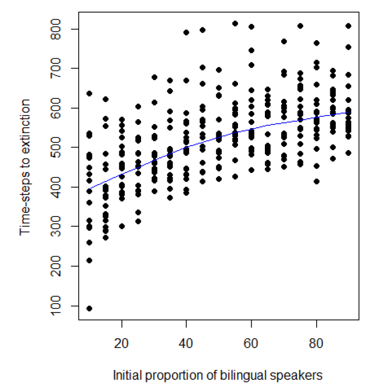
Discussion
On the basis of the analysis of the simulations performed, a number of conclusions can be drawn. I will try to back them up by referring to cases actually observed. It is probably worth starting our discussion with the impact of the exogamy rate of minority-language speakers, i.e. the frequency with which minority people tend to pair and build a family with a non-minority individual. Based on the observed results, exogamous pairing, with the implications in terms of language transmission presented earlier, seems to have a major negative impact on the long-term chances of survival of the minority language. Indeed, numerous authors have observed a substantial negative correlation between the rate of exogamy and the level of minority language intergenerational transmission. For example, Harrison (1999), discussing the case of German immigrants to Canada, observes that a considerable amount of exogamy contributes to a lower level of language maintenance across generations. He compares this with the case of Punjabi-, Chinese- and Spanish-speaking immigrants to Canada, who were characterized by substantially lower rates of exogamy and a higher tendency to pass their language on to the next generation. These trends are confirmed by Frideres (2014), who studied the patterns of intergenerational language transmission among Aboriginal communities in Australia. He observes that within communities with a high a level of exogamy there is a considerably lower use of Aboriginal languages and, consequently, diminished language continuity across generations. Referring to a previous study by Stevens & Schoen (1988), he associated linguistic intermarriage with an instance of group disaffiliation, whose direct effect on the next generation is complete language loss. Finally, Jan et al. (2016) provide further support for this claim by studying the case of Hakka speakers in Taiwan. These findings fit particularly well in our discussion in that, as the authors argue, Hakka minority people are not physically distinguishable from majority people. The distinct Hakka language, along with Hakka traditions and cultures, are the main constituents of the Hakka identity. The authors find that linguistic intermarriage has a significant negative impact on the likelihood of retention of the Hakka language across generations. In particular, they find that exogamy is the single strongest predictor of language loss and that for Hakka people born in mixed (Hakka-Han) families, the likelihood of speaking Hakka decreases by 87% with respect to those who have two Hakka parents.
Moving on to the relationship between education and survival of the minority language community, we could notice that teaching the minority language has a positive impact on the chances of long-term survival and on the level of fluency of speakers. This is especially true if these programs are put in place before the size of the minority community declines too much. The analysis shows that both variables concerning education programs (“education” and “minority threshold”) have a positive impact on the chances of long-term survival of the minority language. However, the impact is not enough to compensate the decline due to higher rates of exogamy. Indeed, they only seem to slow down the decline of the minority language, rather than stop it, let alone reverse it. Sadly, tales of unsuccessful language education programs are quite frequent in the relevant literature, the case of Irish being one of the most famous. To make a list of all the issues that caused Irish revival to be by and large a failure goes well beyond the scope of this article. Numerous authors have already discussed the matter in great detail, such as Lenoach et al. (2012). Here I will only discuss how language education plans can end up being a failure if they are not backed up by the right attitude among the very addressees of the plan. Even if we assume that schooling does make students fluent in the minority language, continuous exposition to majority language and the fact that the majority language might be the first option for many minority-language speakers (i.e., a scenario with a low level of speakers who play the “reveal” strategy), not to mention a low level of mixed households where the minority language is passed on to the next generation, are largely enough to eliminate the benefits of schooling. Already in the nineties, Carnie (1996) mentioned an emblematic issue related to the Irish language revival program, which he labelled a “spectacular failure”. Each year, thousands of English-speaking students with only limited knowledge of Irish participate in language immersion programs at “Gaelic colleges” in the Gaeltacht (the collection of primarily Irish-speaking regions of the Republic of Ireland). However, the massive infusion of English speakers who are reluctant to speak Irish causes the Irish-speaking students to be dramatically outnumbered. As a consequence, English quickly becomes the language of first choice for everyone. This program, rather than pushing English speakers to speak Irish, pushes Irish speakers to speak English.
Conclusions and Potential Developments
The model presented here provides some useful insights into the complex dynamics of language contact and its implications on the decline of minority languages. In particular, it does so by building on a number of relatively simple intuitions on individual language strategies. It considers multiple aspects, which can be combined to create different scenarios. Such scenarios can inform on the variations of the current conditions in the long term and/or on the potential long-term impact of different policies. Consequently, it can be used to serve policy making purposes. It should be noted, however, that I developed and used the model with the final objective of testing the impact of different variables. The idea of creating an in vitro version of a multilingual community and study it derives from the fact that, in real life, it is not possible to observe enough different scenarios with a view to studying the relative impact of each variable. For a practical use, the model would have to be calibrated to reflect the actual case scenario under study and only then it would be able to provide some insights to inform, along with other qualitative and quantitative observations, the process of policy making. Therefore, this model should be seen as a first step towards the higher-level objective of getting language disciplines, social sciences and computational simulation closer together.
As it works through simulations rather than actually observed data, it can be used to estimate the impact of different variables over very long periods of times, which would be otherwise unobservable. Besides, it can be amended or further developed to accommodate all sorts of different settings. For example, should a policy maker want to simulate a specific environment in which behavioural rules are known to work in a different way, she could simply go into the code and modify it accordingly. Alternatively, the model could be extended to abstract and parameterize more behavioural rules, so that they could be switched on and off according to needs. One possible extension could be to change the assumptions concerning education. As said, it is assumed that students involved in language education programs become fluent by the end of schooling. If policy makers have precise data on the average level of fluency reached by students, it could be interesting to modify the model accordingly and look at long-term implications. Clearly, the direct consequences of any lower-than-proficient level at the end of school would result in a reduced effect of education policies. Another extension could be to compare scenarios with different types of reveal-strategy players, to reflect contexts with higher or lower power distance, as discussed in Section 4.14.
On the basis of the previous discussion we can say that the ABM presented in this article provides a reasonably accurate representation of the actual trends of minority language decline resulting from language contact. Indeed, it provided realistic estimates of the trends in the proportions of Romansh-speakers with respect to German speakers in the Canton of Grisons. Besides, several studies confirmed the relative weight of each individual factor included in the model as identified by our analysis. This suggests that the simple behavioural rules that we used to describe individual linguistic strategies of communication and intergenerational transmission are able to capture the essence of people’s actual behaviour. In short, the model found that linguistic intermarriage and the implications assumed by the model in terms of language transmission seem to be the strongest factors affecting the likelihood of long-term survival of minority languages, while factors such as language education and the willingness to speak the minority language seem to have only a marginal impact. Higher levels of exogamy are associated with quicker rates of decline of the minority language. On the contrary, all the variables included in the model seem to have a non-negligible impact on the level of fluency of minority-language speakers.
Needless to say, promoting endogenous marrying is not an advisable solution, nor is forcing people to speak the minority language. Rather, an answer to the decline of minority languages could lie in the social perception of these languages. The strong impact of the exogamy rate variable is mostly due to the assumed consequences of exogamy, i.e. that children born to mixed couples do not learn the minority language. The ABM presented in this paper reveals the importance of language choice in exogamic couples. As I explained, the simulations assume that in bilingual couples, the home language will be the majority one. This can be amended to reflect other possibilities, in which, for example, mixed families are actually encouraged to pass both languages on to the next generation. Or else, it could be assumed that majority-llanguage speakers learn the minority language if their partner speaks it. This might easily hedge the decline of the minority language community, if not reverse it.
A more positive social attitude towards minority languages, which may result from measures such as granting the status of official language or supporting cultural activities, could improve the chances of long-term survival. Indeed, it could:
- influence communication dynamics in mixed families, pushing the monolingual parent to learn the minority language, raise the children bilingually and make sure that they become fluent in the minority language;
- increase the likelihood that a minority language speaker reveals that she speaks the minority language.
These two effects combined could have a significant impact on the long-term survival of minority languages. Indeed, attitude and social perception seem to play an important role in the dynamics of minority languages and that any measure in support of these languages risks being a failure if it is not welcomed by individuals with a positive attitude. As a matter of fact, success stories of this kind already exist. Ever since the end of Francoism, many institutional campaigns have been launched to support the revitalization of the Catalan language in Catalan-speaking regions of Spain. For example, the Government of Catalonia started many initiatives that explicitly addressed the issue of people feeling ashamed to speak Catalan. One of them was the “Dóna corda al català” (“Unleash the Catalan language”) campaign, which was articulated in three themes: “Parla sense vergonya”, “Parla amb llibertat” and “Per començar, parla en català”, which roughly translate to “Don’t feel ashamed to speak”, “Speak freely” and “Speak Catalan from the outset,” respectively[20].
These campaigns were further supported by the introduction of Catalan as a preferential language for education and by the creation of Catalan-speaking media.
We can also expand our discussion to speculate on the implications of opening up to migration dynamics. In particular, we could consider the case of immigration flows and the issue of language choice for immigrants. As Chiswick & Miller (1994) note, the choice is straightforward for individuals migrating to monolingual countries. However, a number of variables come into play when the destination country is multilingual. These variables include proximity to the immigrant’s native language, the predominant language in the specific region where they settle and its relative weight on the labour market. Considering these variables, it is easy to see that significant migration flows can have an impact on the size of minority language community, either positive or negative. For example, it is no secret that, among other things, massive immigration of French-speakers and other immigrants who preferred French over Dutch, combined with the perception of French as an elite language, is one of the factors that made Brussels, a historically Dutch-speaking area, into a French-majority city (Leclerc 2008).
It should be noted that education programs, as conceived in our ABM, were only addressed to individuals in school age. They are then left to normal communication dynamics for the rest of their life, with the implications in terms of fluency in the minority language explained above. One way to increase the impact of education could be to introduce lifelong learning programs, so that the level of fluency of minority-language speakers could be sustained also after school age in spite of continuous exposition to the majority language. Besides, one could also think of extending minority language education programs to majority-llanguage speakers, whether they have a majority-majority or a mixed majority-minority background. This would easily amplify the impact of the two education-related variables.
Finally, concerning the relationship between vitality, defined as the proportion of people able to speak the minority language, and the long-term survival of the minority language, we saw that the initial proportion of bilingual speakers is only weakly correlated with long-term survival, and that this correlation is virtually non-existent for initial proportions greater than 40%. This finding is somehow comforting, in that it implies that the long-term survival of the minority language community is highly dependent on other factors. This means that it is possible to improve the vitality of minority languages through “policy-actionable” variables, almost regardless of the current proportion of minority-language speakers.
Notes
- For an in-depth discussion on the transversal character of language issues, see Grin et al. (2014).
- Examples are numerous and include simulations of social identity dynamics leading to group formation (Smaldino et al. 2012), the evolution of grammar and vocabulary (Lekvam et al. 2014, Sierra-Santibáñez 2014), and income distribution and wealth accumulation across different social classes (Russo 2017).
- Note that Appel & Muysken (2005) speak of the case of two languages, but their categorization can be easily extended to the case of more than two languages.
- It should be noted that articles 4 and 70 of the Swiss Constitution simply speak of “German” (Deutsch) as being a national and official language, but it is normally interpreted to mean “High German” (Hochdeutsch), which is also informally referred to as the “written language” (Schriftsprache) in the Swiss context. This applies also to the French, Italian and Romansh (equally official) versions of the Constitution.
- From here on, I will use the term “German” to refer indifferently to High German and Swiss German.
- For a review of the various definitions of “bilingualism”, see Paradowski & Bator ( 2018).
- There are numerous studies that show how languages (or varieties thereof) can be associated with a more or less favourable perception in certain contexts. For example, see Garcia (1984) for a discussion on the different perception of Castillian-speakers and Valencian-speakers in the Valencian Community in Spain.
- A rather different kind of support for the idea of higher-status male-specific language transmission is provided by Forster & Renfrew (2011). They found that prehistoric language death and replacement correlates with immigration of males but not necessarily females, according to a global analysis of modern mtDNA (which is inherited from mothers only) and Y chromosomal patterns. This suggests that prehistoric women may have preferred to adopt and pass on the language of immigrant males, especially if they displayed military prowess or a perceived higher status, yielding the language/Y-chromosome correlation observed today.
- Another example of such behaviour is presented in a study by the Canadian office of statistics on language use in different family configurations (see https://www150.statcan.gc.ca/n1/pub/75-006-x/2015001/article/14301-eng.pdf). In short, the study shows that in communities where both French (minority) and English (majority) are spoken, families in which both parents have French as a mother tongue are much more likely to use French as a home language than English, as opposed to couples where only one parent has French as his/her main language.
- For more on communication accommodation theory, see Giles (2008).
- “Romansh” is actually a collection of five mutually understandable Romance languages, each with its own written standard. They belong to the same language sub-family as Ladin and Friulan, which are spoken in Northern Italy. In 1982 a unified Romansh language with a shared written and spoken standard was introduced by the Lia Rumantscha (Romansh League), called Rumantsch Grischun (Grisons Romansh).
- These numbers were calculated using data published in Coray (2008).
- https://data.worldbank.org/country/switzerland.
- The two options in German were “Hauptsprache” and “Umgangssprache.” Another possible translation for “Umgangssprache” could be “language of social interaction.”
- The value of zero was selected to simulate the impact of absence of policy. Values over 50% would have skewed the results, in that values from 50% to 100% are all above the initial proportion of minority speakers.
- Technically, as explained earlier, the range is not from 0 to 100 (or 0 to 50 for minority threshold), but from -50 to 50 (and -25 to 25 for minority threshold). Indeed, in order to account for the potential collinearity between linear and quadratic terms, the variables were centered on their mean, as it is customary in these cases. This does not imply any difference in interpretation. For more on this, see Afshartous & Preston (2011).
- The odds of an event \(y\) are defined as \(\frac{p(y)}{1-p(y)}\) where \(p(y)\) is the probability of said event. For example, the probability of rolling a (fair) die and getting a 4 is 1/6, while the odds of the same event is 1 to 5, that is, if we roll a die many times, we would expect to get a 4 every 5 times the roll gives any other outcome.
- The words "positive" and "negative" are clearly not meant as synonymous with, respectively, "desirable" and "undesirable."
- The combined impact of the variation in two factors is computed by multiplying the two exponentiated coefficients. Indeed,
- Examples can be found at the following addresses: https://www.youtube.com/watch?v=XlH4ZLSi3YM,https://www.youtube.com/watch?v=rtjniMmgY5A, https://www.youtube.com/watch?v=2wBmCrvj7Iw.
| $$\frac{exp(\beta_0+\beta_1(x_1+1)+\beta_2(x_2+1))}{exp(\beta_0+\beta_1x_1+\beta_2x_2)}=e^{\beta_1+\beta_2}=e^{\beta_1}e^{\beta_2}$$ |
Acknowledgements
I would like to thank Mr Tesar and Mr Ullmann of the Swiss Federal Statistical Office for their availability to provide the data on the linguistic profile of households in the canton of Grisons. I would also like to thank my colleague Dr Albert Morales (Faculty of Translation and Interpretation, University of Geneva) for consulting extensively on the policies in support of the Catalan language and for reviewing the translation of the Catalan text. Finally, I would like to thank Professor Clau Solèr (University of Geneva) for consulting in depth on the sociolinguistics of Romansh. The research leading to these results has received funding from the European Community’s Seventh Framework Programme under grant agreement No. 613344 (Project MIME) and from the Swiss National Science Foundation.Model Documentation
The model was programmed using NetLogo 6.0 and the code is available at: https://www.comses.net/codebases/3108c3b3-ed14-487d-999a-c85b7a12256a/releases/1.0.0/.References
ABRAMS, D. M., & Strogatz, S. H. (2003). Linguistics: Modelling the dynamics of language death. Nature, 424, 900. [doi:10.1038/424900a]
AFSHARTOUS, D., & Preston, R. A. (2011). Key results of interaction models with centering. Journal of Statistics Education, 19(3). 1-24. [doi:10.1080/10691898.2011.11889620]
APPEL, R., & Muysken, P. (2005). Language Contact and Bilingualism. Amsterdam: Amsterdam University Press.
BILLARI, F. C. (2015). Integrating macro-and micro-level approaches in the explanation of population change. Population Studies, 69(sup1), S11-S20. [doi:10.1080/00324728.2015.1009712]
BROWN, P., Levinson, S. C., & Levinson, S. C. (1987). Politeness: Some Universals in Language Usage (Vol. 4). Cambridge, MA: Cambridge University Press. [doi:10.1017/cbo9780511813085]
CARNIE, A. (1996). Modern Irish: A case study in language revival failure. Papers on Language Endangerment and the maintenance of linguistic diversity, 99-114.
CARSON, J. (2002). Verification validation: model verification and validation. In Proceedings of the 34th conference on Winter simulation: exploring new frontiers (pp. 52-58). Winter Simulation Conference. [doi:10.1109/wsc.2002.1172868]
CASTELLÓ X., Loureiro-Porto, L., & San Miguel, M. (2013). Agent-based models of language competition. International Journal of the Sociology of Language, 221, 21–51. [doi:10.1515/ijsl-2013-0022]
CHISWICK, B. R., & Miller, P. W. (1994). Language choice among immigrants in a multi-lingual destination. Journal of Population Economics, 7(2), 119-131. [doi:10.1007/bf00173615]
COLEMAN J. (1990). Foundations of Social Theory. Cambridge: Harvard University Press.
CONKLIN, N. F., & Lourie, M. A. (1983). A Host of Tongues: Language Communities in the United States. New York: Free Press.
CORAY, R. (2008). Von der Mumma Romontscha zum Retortenbaby Rumantsch Grischun. Bündner Monatsblatt.
CRAWFORD, V. P., & Sobel, J. (1982). Strategic information transmission. Econometrica: Journal of the Econometric Society, 1431-1451.
DE FLAUGERGUES A. (2016). Pratiques linguistiques en Suisse Premiers résultats de l’Enquête sur la langue, la religion et la culture 2014. Report, Neuchâtel: Office fédéral de la statistique.
FORSTER, P., & Renfrew, C. (2011). Mother tongue and Y chromosomes. Science, 333(6048), 1390-1391. [doi:10.1126/science.1205331]
FRIDERES, J. (2014). 'Continuity or disappearance: Aboriginal languages in Canada.‘ In F Trovato & A Romaniuk (eds), Aboriginal Populations: Social, Demographic, and Epidemiological Perspectives. Edmonton: The University of Alberta Press, pp. 303–324.
FURER, J. J. (2005). Die Aktuelle Lage des Romanischen. Office fédéral de la statistique.
GABBRIELLINI, S. (2018). Why you need to know about agent-based modelling. Available at: https://www.linkedin.com\\/pulse/why-you-need-know-agent-based-modelling-simone-gabbriellini/.
GANGULY, C., Ray, I. (2012). Simple Mediation in a Cheap-Talk Game. Department of Economics Discussion Paper 05-08RRR, University of Birmingham, UK.
GILES, H., Bourhis, R. Y., & Taylor, D. M. (1977). ‘Towards a theory of language in ethnic group relations.’ In H Giles (ed), Language, Ethnicity, and Intergroup Relations. New York: Academic Press, pp. 307–349.
GILES, H. (2008). ‘Communication accommodation theory: “When in Rome…” or not!’ In Baxter LA and Braithewaite DO (eds) Engaging Theories in Interpersonal Communication. Thousand Oaks, CA: Sage, pp. 161-173. [doi:10.4135/9781483329529.n12]
GRIN, F. (1990). The economic approach to minority languages. Journal of Multilingual & Multicultural Development, 11(1-2), 153-173. [doi:10.1080/01434632.1990.9994406]
GRIN, F. (1992). Towards a threshold theory of minority language survival. Kyklos, 45(1), 69-97. [doi:10.1111/j.1467-6435.1992.tb02108.x]
GRIN, F. (2003). Language Policy Evaluation and the European Charter for Regional or Minority Languages. Berlin Heidelberg: Springer. [doi:10.1057/9780230502666]
GRIN, F. (2016). ‘Challenges of Minority Languages.’ In Ginsburg V and Weber S (eds) The Palgrave Handbook of Economics and Language. New York: Palgrave MacMillan, pp. 616-658. [doi:10.1007/978-1-137-32505-1_22]
GRIN, F., Marácz, L., Pokorn, N. K., & Kraus, P. A. (2014). Mobility and inclusion in multilingual Europe: A position paper on the MIME Project. Available at: http://www.mime-project.org/resources/MIME-POSITION-PAPER-V4.pdf. [doi:10.1515/eujal-2018-0013]
GRIN, F., Sfreddo, C., & Vaillancourt, F. (2010). The Economics of the Multilingual Workplace. London, UK: Routledge.
GROW, A. (2017). ‘Regression metamodels for sensitivity analysis in agent-based computational demography.’ In Grow A., Van Bavel J. (eds), Agent-based Modelling in Population Studies . Cham: Springer, pp. 185-210. [doi:10.1007/978-3-319-32283-4_7]
HARRISON, B. R. (1999). ‘Intergenerational Language Learning.’ In Halli SS and Driedger L (eds), Immigrant Canada: Demographic, Economic, and Social Challenges. Toronto: University of Toronto Press, pp. 307-320. [doi:10.3138/9781442676022-016]
HEDSTRÖM, P., & Swedberg, R. (1998). ‘Social mechanisms: An introductory essay.’ (eds), Social Mechanisms: An Analytical Approach to Social Theory. Cambridge, MA: Cambridge University Press, pp. 1-31. [doi:10.1017/cbo9780511663901.001]
HOFSTEDE, G. (2011) Dimensionalizing Cultures: The Hofstede Model in Context. Online Readings in Psychology and Culture, 2(1). Available at: https://scholarworks.gvsu.edu/orpc/vol2/iss1/8/. [doi:10.9707/2307-0919.1014]
HORNBERGER N. H. (2010). ‘Language Shift and Language Revitalization.’ In B. Kaplan (ed), The Oxford Handbook of Applied Linguistics, (2 ed.). Oxford: Oxford University Press, pp. 365-373. [doi:10.1093/oxfordhb/9780195384253.013.0028]
ISERN , N., & Fort, J. (2014). Language extinction and linguistic fronts. Journal of the Royal Society Interface, 11(94), 20140028. [doi:10.1098/rsif.2014.0028]
JAN, J. S., Kuan, P. Y., & Lomeli, A. (2016). Social context, parental exogamy and Hakka language retention in Taiwan. Journal of Multilingual and Multicultural Development, 37(8), 794-804. [doi:10.1080/01434632.2016.1142551]
KREAGER, P. (2015). Population and the Making of the Human Sciences. Population in the Human Sciences: Concepts, Models, Evidence, 55. [doi:10.1093/acprof:oso/9780199688203.003.0002]
LECLERC, J. (2008). Histoire de la Belgique et ses conséquences linguistiques. Université Laval. Available at: http://www.axl.cefan.ulaval.ca/europe/belgiqueetat.
LEKVAM, T., Gambäck, B., & Bungum, L. (2014, April). Agent-based modeling of language evolution. In Proceedings of the 5th Workshop on Cognitive Aspects of Computational Language Learning (CogACLL), pp. 49-54. [doi:10.3115/v1/w14-0510]
LENOACH, C., Ó Giollagáin, C., & Ó Curnáin, B. (2012). An Chonair Chaoch: An Mionteangachas sa Dátheangachas. Vearsa.
LÜDI, G., Werlen, I., Franceschini, R., Antonini, F., Bianconi, S., Furer, J. J., Quiroga-Blaser, C., Wymann, A. (1997). Le paysage linguistique de la Suisse. Recensement fédéral de la population 1990. Report. Berne: Office fédéral de la statistique.
MILROY, L. (1980). Language and Social networks. Oxford: Blackwell.
MINETT, J. W., & Wang, W. S. (2008). Modelling endangered languages: The effects of bilingualism and social structure. Lingua, 118(1), 19-45. [doi:10.1016/j.lingua.2007.04.001]
NELDE, P. (2010). ‘Language Contact.’ In Kaplan RB (ed), The Oxford Handbook of Applied Linguistics, (2 ed.). Oxford: Oxford University Press, pp. 325-334.
OSSWALD, S. E. (1988). Stabilitätsmindernde Faktoren bei einer sprachlichen Minderheit: Die Rätoromanen in Graubünden. PhD Thesis, University of Hannover, Germany.
PARADOWSKI, M. & Bator, A. (2018). Perceived effectiveness of language acquisition in the process of multilingual upbringing by parents of different nationalities. International Journal of Bilingual Education and Bilingualism, 21(6), 647-665. [doi:10.1080/13670050.2016.1203858]
PATRIARCA, M., Castelló, X., Uriarte, J. R., Eguíluz, V. M., & San Miguel, M. (2012). Modeling two-language competition dynamics. Advances in Complex Systems, 15(03n04), 1250048. [doi:10.1142/s0219525912500488]
GARCIA, M. R. (1984). Speech attitudes to speakers of language varieties in a bilingual situation. International Journal of the Sociology of Language, 47, 73-90.
RUSSO, A. (2017). An Agent Based Macroeconomic Model with Social Classes and Endogenous Crises. Italian Economic Journal, 3(3), 285-306. [doi:10.1007/s40797-017-0060-4]
SIERRA-SANTIBÁÑEZ, J. (2014). An agent-based model studying the acquisition of a language system of logical constructions. In Twenty-Eighth AAAI Conference on Artificial Intelligence, 1, 350-357.
SMALDINO, P., Pickett, C., Sherman, J., & Schank, J. (2012). An agent-based model of social identity dynamics. Journal of Artificial Societies and Social Simulation, 15(4), 7: https://www.jasss.org/15/4/7.html. [doi:10.18564/jasss.2030]
SOLÈR, C (2004) Le Rhéto-Romanche en Suisse. Bilinguisme et diglossie: problèmes et propositions. Education et Sociétés Plurilingues 16: 15-26.
SOLÈR, C. (2015). Sociolinguistique et standardisation romanche. Class notes, University of Geneva, Switzerland.
SPERLICH, S., & Uriarte, R. (2014). Economics and (Minority) Language: Why is it so hard to save a threatened language? Ikerlanak, IL 77/14. University of the Basque Country, Mimeo.
STEVENS, G., & Schoen, R. (1988). Linguistic intermarriage in the United States. Journal of Marriage and the Family, 267-279. [doi:10.2307/352445]
THOMASON, S. G. (2001). Language Contact. Edinburgh: Edinburgh University Press.
URIARTE, J. R. (2016). ‘A Game-Theoretic Analysis of Minority Language Use in Multilingual Societies.’ In V Ginsburgh, S Weber, P Macmillan (eds), The Palgrave Handbook of Economics and Language . London: Palgrave Macmillan, pp. 689-711. [doi:10.1007/978-1-137-32505-1_24]
VAN BAVEL, J., & Grow, A. (2017). ‘Introduction: Agent-based modelling as a tool to advance evolutionary population theory.’ In A Grow & J Van Bavel (eds), Agent-Based Modelling in Population Studies. Cham: Springer, pp. 3-27. [doi:10.1007/978-3-319-32283-4_1]
WILENSKY, U., & Rand, W. (2015). An Introduction to Agent-Based Modeling: Modeling Natural, Social, and Engineered Complex Systems with NetLogo. New York, NJ: MIT Press.
WILLIAMS, R. A. (2018). Lessons learned on development and application of agent-based models of complex dynamical systems. Simulation Modelling Practice and Theory, 83, 201-212. [doi:10.1016/j.simpat.2017.11.001]
ZHANG, M., & Gong, T. (2013). Principles of parametric estimation in modeling language competition. Proceedings of the National Academy of Sciences, 110(24), 9698-9703. [doi:10.1073/pnas.1303108110]
ZIPF, G. K. (1949). Human Behavior and the Principle of Least Effort. An Introduction to Human Ecology. Oxford, England: Addison-Wesley Press.