
Introduction
The agricultural water cycle involves a large proportion of water resources, accounting for approximately 70 % of global water withdrawals (FAO 2016). In a foreseeable future of growing population and changing climatic conditions, where agriculture will have to increase its production some 50 % by 2050, those requirements are not likely to diminish (FAO 2017). These expectations shall produce increasing socio-economic stress on the water cycle unless sound policy is implemented and effective actions are taken.
There is widespread consensus that water could be better managed in agriculture, especially where traditional low-efficiency irrigation systems are commonly used (see López-Gunn et al. 2012b). Consequently, many stakeholders consider the modernisation of irrigation systems as an essential means for better water use in farmers communities —and also for promoting other social values such as rural development and environmental sustainability.
The motivation behind this paper is to understand how modernisation takes place in such communities in order to provide input for policy-design. We intend to model policies in the water domain and it is therefore necessary to model different decision processes and profiles of stakeholders. We model Spanish “irrigation communities” (ICs) because they use a large share of water resources in Spain, because enough reliable data from some communities is available to set up a core working model that may be extended to other communities, and because they follow an innovation process that may be adapted to agricultural communities elsewhere.
Our approach is to build a simple agent-based model (ABM) —a population of farmer agents and a socio-economic context that influences individual choices— to understand how the dispositions of individuals to modernise propagate in the community and end up in the actual adoption or rejection of the innovation (Section 2). In our model, individual decision-making is based on comparing the current farm performance against the expected return (see Knox et al. 2012), as well as taking social influence into account.
The model we discuss here explains a two-staged adoption of modern irrigation technology —collective and individual— with profit-driven individuals immersed in a social network where farm extension is a proxy for social influence (Section 3). We model individual decisions (unknown from data) from which we simulate community adoption, which fits quite faithfully the actual adoption data. We calibrated our model with real data from two communities and found that, in these cases in which agriculture is market-oriented and water scarcity is high, favourable modernisation conditions arise from added-value crops, which are enabled by higher water allocations and greater irrigation efficiency (Section 4).
This work presents a particular case in the water policy domain that, approached with ABM, allows the exploration of alternative policies (see Srinivasan et al. 2017). It also suggests the need of a richer socio-cognitive model (of individuals and communities) to explain modernisation in other types of communities (Sections 5 and 6).
Background and State of the Art
Modernisation of irrigation systems is said to improve water use efficiency (see López-Gunn et al. 2012b). In traditional communities, water is distributed by means of open channels, and applied using field ditches. A drawback of such systems is their significant level of water losses. These contrast with modern systems with pressurised networks and sprinklers or drip pipes —whose adoption is known as “modernisation”—, that minimise water losses but consume more energy.
An irrigation community (IC) is a group of agents that share a water allocation right, whose main use is farm irrigation. In Spain, an IC has the power to plan and execute infrastructure projects, as long as an assembly constituted by all its members agrees. This procedure is based on direct voting, for which farmers hold a number of votes proportional to their farm extension. Actual modernisation of an IC (our object of simulation) is a two-stage process: (i) the community upgrades the shared infrastructure only when supporters of modernisation gather enough votes to pass the project; and (ii) only then are farmers able to install drip or sprinkler systems in their own fields.
Diffusion of innovations is the process through which practices, ideas or products, are spread and adopted over time within a social system (Rogers 1995). Diffusion of innovations in ICs has been studied using equation-based models (Alcón 2007). However, this modelling approach does not reflect agent heterogeneity and does not reproduce farmers’ social interactions explicitly.
Agent-based models can overcome these limitations and have been used to study adoption of innovations (Deffuant et al. 2005; Sengupta et al. 2005; Zhang et al. 2016; Deffuant et al. 2002). Moreover, as we present in this paper, it allows to approach adoption-decision as a contingent phenomena, in which farmers may adopt a technology individually only after a prior collective agreement that emerges from the same decision-making units. As Hu et al. (2017) indicate, major challenges in modelling behaviour in AMB is data scarcity and consider a proper representation of bounded rationality implications in the domain and context under study. They propose that working from domain experts’ knowledge may help to address such challenges, as we did in this work.
ABM has been also used to explore human social behaviour in the agricultural domain (Huber et al. 2018; Berger 2001; Schreinemachers & Berger 2011), although it has been used for answering research questions related to land-use changes (Parker et al. 2003) and implementation of payment for ecosystem services (Sengupta et al. 2005; Chen et al. 2012).
A line in the agricultural domain has taken a socio-hydrology approach (Sivapalan et al. 2014), combining human behavioural models with biophysical models, to focus, in particular, on water issues. Becu et al. (2003) presented the CATCHSCAPE model, whose central point was the impact of upstream agricultural water management on the farming activity downstream, for which they considered a spatial representation of the watershed explicitly. Hu et al. (2017) explored the use of groundwater for irrigation, and introduced environmental, economic, social, and infrastructure aspects on agents’ decision-making on groundwater pumping. They concluded that factors relevant in agents’ decisions were temperature, precipitation, groundwater level and crop prices —variables that are reflected in our work in water availability and climatologic conditions. However, that model lacked social interaction between agents, since the agents represented aggregation of multiple farmers.
Similar to the work we present, Holtz & Pahl-Wostl (2012) used ABM to conduct historical research in a Spanish basin where irrigation agriculture was a key economic activity. However, they focused on land-use changes and groundwater use. They considered diffusion of irrigation technologies, multiple crop options, and cognitive biases as risk aversion and concluded that farmer models should consider more values than profit orientation (e.g. lifestyle).
Berger (2001) developed a model for assessing different policy scenarios in the diffusion of innovations and resource use changes. The model was based on a cellular automata modelling approach, since it was considered that spatial dimension was essential in agriculture models. Although some of the potentialities afforded by the spatial representation are not included in our model (e.g. resource distribution, nutrient diffusion, return flows, etc.), they are easy to be implemented in future work, since the spatial dimension is already taken into account.
The usual approach of innovation-diffusion models base decision-making on utility functions (Kiesling et al. 2012), and also consider contagion processes (Alcón 2007; Holtz & Pahl-Wostl 2012; Berger 2001). Although other non-economic variables might be included in this function, it is assumed that most farmers (especially large-scale farmers) focus primarily on economic utility as the driving value (Benouniche et al. 2014). For instance, Sengupta et al. (2005) categorised farmers according to their motivation, distinguishing between large-scale farmers that pursued profit maximisation and small-scale farmers interested in conservation of rural lifestyle. In this paper we identify a class of ICs for which the profit-driven assumption is plausible, due to the regional socioeconomic context. Nonetheless, we recognise the need of considering additional values and interests (see Huber et al. 2018).
To our knowledge, modernisation of irrigation systems has not been modelled as a two-stage contingent process in ABM, where relationships between individuals and the emergence of collective properties is essential. This work, particularly, addresses this gap, and relates adoption decision both at the individual and collective level to agricultural and water economy aspects.
Model
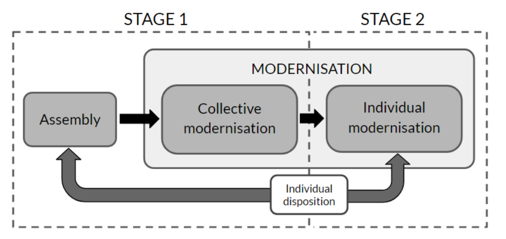
The model we present here represents an irrigation community (IC) as a set of farmer agents for which modernisation is achieved in two stages (Figure 1). The first one accounts for the commitment of collective modernisation, in which each farmer evaluates whether it is worth modernising its farm, and then, all farmers need to reach a collective agreement based on an aggregation of their attitudes. In the subsequent second stage, once the community agrees to modernise, individual farmers may choose to modernise their own farms. We draw upon information from experts and field data from irrigation communities to design and calibrate the model. We model individual decisions (unknown from data) from which we model community adoption (comparable with actual adoption data). Thus, the model can be used to gauge the proclivity of a given community to modernise and reveals external actions that may induce modernisation.
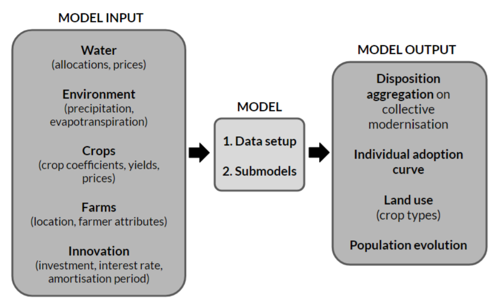
We use five types of data, drawn from several sources, as input for the model (Figure 2, Appendix B). We obtain, as a raw outcome, the individuals’ disposition to modernise (Stage 1) and their actual adoption (Stage 2), that we aggregate to obtain the collective disposition and the adoption curve, respectively. We use NetLogo as a simulation platform.
Entities and assumptions
Farmers are the only kind of agent in the model. They are characterised by the following attributes: (i) farm area; (ii) farm location; (iii) supply support (capability to increase water supply by means of alternative sources, such as private wells); (iv) crop-inertia (reluctance to change crops in spite of potential profitability); (v) risk-aversion; (vi) age; (vii) capital; (viii) past revenue (economic outcome of the past agricultural season); and (ix) disposition towards modernisation. Attributes (i–vi) are based on real-data (see Appendix B) and attributes (vi–ix) evolve as results of the simulation[1].
Social influence is a key element in the modernisation process, since farmers use information from other farmers to make decisions. Nonetheless, the replication of social networks in such agricultural communities is not a trivial task: social interaction between farmers may happen in multiple occasions (e.g. community assemblies, sporadic contact in town, familiar relationships, etc.). Indeed, this particular phenomena justifies more fieldwork.
In our model, we based farmers’ social network on two elements: (i) spatial proximity and (ii) farm scale. Although spatial proximity (i.e. social distance) generation model may ignore some aspects that are relevant in social networks (for instance, that well-connected nodes are generally connected with each other), we considered it to be a plausible hypothesis for constituting a social network in an agricultural community. Hamill & Gilbert (2009) proposed a similar mechanism to generate social networks, whose perception model is based on social circles (whose radius was labelled ‘social reach’).
We introduced homophily in the social network with the consideration of the farm scale. The assumption is that each farmer pays attention to similar neighbours, since their plots have similar farming features and their experiences are likely to apply. Scale is defined on farm extension, following the classification of Román-Cervantes (1996) in Spanish communities: (i) small scale farmers are those that own between 0 and 20 hectares; (ii) medium scale, from 20 to 70 ha; and (iii) large scale, greater than 70 ha. Following experts’ opinion and Benouniche et al. (2014), we assume that all farmers may be linked but small scale and large scale farmers do not influence each other.
Formally, farmer i and farmer j of the set of farmers A are connected \(R(i,j)\) when the distance between them is below a maximum distance \(d_{max}\) and their farm scales are not small and large (Expr. 1). The social network \(N_{i}\) of the farmer i (the other farmers it is connected with) is given by Expr. 2. Note that social network \(N_{i}\) is defined at the initialisation step of the simulation and fix for the whole simulation.
| $$\small{ \begin{split} (\forall i, j \in A )(R(i,j) \leftrightarrow (distance(i,j) \leq d_{max}) \wedge \\ \neg (scale(i)=\text{small}\wedge scale(j)=\text{large}) \wedge( i\neq j)) \end{split} }$$ | (1) |
| $$\label{eq:network} \small{ \forall i \in A, \, N_i = \{j \in A : R(i,j) \} }$$ | (2) |
Farmers have dichotomous states in three issues: (i) farming their lands and participating in the community (active or inactive); (ii) adoption of the innovation (traditional or modernised); and (iii) attitude towards modernisation (willing to modernise or not willing to modernise). A farmer willing to modernise will vote for collective modernisation in Stage 1 and will modernise its individual plot if possible in Stage 2. Notice that willingness is a state, whose transition is determined by the disposition as explained below (Equation 6).
To start a simulation, all farmers start being active, traditional, not willing to modernise, and have the crop that best suits their initial water availability.
The spatial scale of the model represents the farming area of the community. The model simulates decades of activity through discrete one-year steps, although some submodels use one-month steps (for instance, the crop yield estimation considers one-month steps). All the submodels are explained in detail in Appendix A and data in Appendix B.
Process overview
The following procedures are executed sequentially each time-step (one year) (See Appendix A for further details):
- Update allocation: set water context variables, such as water allocation and water prices.
- Water availability: determined by the water allocated to the farmer, expected rainfall, private water supply (wells), and the efficiency of the irrigation system (shared and individual irrigation infrastructure).
- Crop choice: farmers choose one crop (from a list of options), aiming to maximise their income. For the sake of simplicity, crop choice depends only on water and crop-related variables. Crop water requirements are calculated as the reference evapotranspiration multiplied by a crop coefficient (see Allen et al. 1998).
- Update environment: precipitation and evapotranspiration are updated and memorised by farmers to choose crops next year.
- Production: Revenue := Income - Cost: Income is a function of crop market prices, farm area, and crop yield, which is adjusted according to water stress (see Steduto et al. 2012). Cost adds up the costs of water, energy, farm inputs and amortisation of the individual’s irrigation system.
- Activity?: farmers decide whether to stop farming or not depending on the revenue and the capital they have.
- Modernisation? (only Stage 1): farmers’ willingness to modernise is defined by two processes: individual decision-making and social influence.
- Assembly (only Stage 1): farmers vote for or against collective modernisation.
- Modernise (only Stage 2): those farmers who are willing to modernise their farms do so. There is no strict dependency of this decision and what the farmers voted in the assembly.
- Population evolution: farmers that reach the retirement age trigger a generational replacement, and inactive farmers can become active again, transfer their land to a new farmer, or remain inactive.
Submodels
Stage 1: The community commits to modernise
Individual decision-making: It is based on opportunity costs of traditional systems. Taking into account that modernisation would have brought a higher volume of available water, farmers evaluate how it would have affected their economy. Revenue and expectation are calculated as the difference between income and costs (Equations 3 and 4). In this specific procedure, past revenue considers the traditional irrigation system (shared and individual), whereas expectation regards a modernised system. Collective adoption costs are introduced as water costs (i.e. tariff scheme), whereas individual costs are those of amortisation. These variables are different in each time-step t, depending on the decisions made by the farmer i and context variables.
| $$\small{ PastRevenue_{i,t} := Income_{i,t} - Costs_{i,t} }$$ | (3) |
| $$\small{ Expectation_{i,t} := Income_{i,t}^{(modernised)} - Costs_{i,t}^{(modernised)} }$$ | (4) |
Farmers must perceive that the utility of the expectation is greater than the past revenue (Equation 5). Provided that this condition is met, disposition compares expectation and past revenue including a risk-aversion parameter \(\gamma_{S1}\) (Equation 6). This parameter is greater than or equal to zero; when it is zero, the farmer has no risk aversion and will adopt the innovation as long as benefits are expected; on the contrary, a large value for this parameter means that the farmer is averse to changes and will adopt only if it entails significant profits. As the disposition ranges from zero to one, a negative result will be considered as zero.
| $$\small{ Expectation_{i,t} \geq PastRevenue_{i,t} }$$ | (5) |
| $$\small{ Disposition_{i,t} := 1 - \gamma_{S1} \frac{PastRevenue_{i,t}}{Expectation_{i,t}} }$$ | (6) |
Social influence: a farmer i receives an influence on its own disposition. The new disposition is the weighted average of the disposition of its neighbours (i.e. the agents that constitute \(N_{i}\)), besides its own disposition prior the influence. The weights are determined proportionally to their farm area (namely, their farm area \(Area_{j}\) divided by the total area \(Area_{T}\) of the farmers in \(\{N_{i}\}\cup\{i\}\)) (Equation 7).
| $$\small{ Disposition_{i,t} := \sum_{j}^{\{N_{i}\}\cup\{i\}} \frac{Area_{j}}{Area_{T}} \cdot Disposition_{j,t} }$$ | (7) |
State transition: Each year, the transition from not willing to modernise to willing to modernise is based on a probability \(P_{t}\) (Equation 8). This transition is bidirectional, meaning that farmers can change their mind on whether to modernise or not. If the farmer was already willing to modernise (W ), the complementary probability is used as the transition probability.
| $$\small{ P_{t}[\,W\,|\,\neg W\,] := Disposition_{t} \qquad P_{t}[\,\neg W\,|\,W\,] := 1 - Disposition_{t} }$$ | (8) |
Assembly: The community will commit to modernise only when more than half the votes are for modernising (that is, all farmers may cast their votes but only farmers who are active and willing to modernise vote in favour). The number of votes each farmer has is proportional to its farm area.
Stage 2: Individuals modernise their plots
Individual decision-making: The procedure is the same as in the Stage 1, except that the risk-aversion parameter \(\gamma_{S2}\) is now greater than before. According to expert’s observations, in the first stage farmers do not have to commit to adopt; and, furthermore, collective costs are shared among all community members. However, in Stage 2 farmers will invest their own money in their own plot that they will eventually have to pay with their own income. Therefore, their commitment is more fragile.
Social influence: it is based on imitation. Farmers who have not adopted observe those farmers in their social network \(N_{i}\) who have already adopted and also are making a profit (Expr. 9) —thus, they use a temporary social network \(\hat{N}_{i,t}\). Then, they calculate an expected income from the average revenue per unit of area (Equation 10). More precisely, a farmer i at time-step t:
| $$\small{ \hat{N}_{i,t} = \{j \in N_{i} : (Modernised(j)=\text{true}) \wedge (PastRevenue_{j,t}>0) \} }$$ | (9) |
| $$\small{ Expectation_{i,t} := Area_{i} \cdot \bigg[ \frac{1}{|\hat{N}_{i, t}|} \cdot \sum_{j}^{\hat{N}_{i, t}} \frac{PastRevenue_{j,t}}{Area_{j}} \bigg] }$$ | (10) |
Expectation must meet the previous condition (Equation 5). Afterwards, a transition probability is calculated as before (Equation 6), but using a specific imitation risk-aversion parameter \(\alpha_{t}\). This parameter decreases over time because, as time passes, knowledge about the innovation (both internal and external to the community) is higher, and imitation is less risky. This is represented by a reduction parameter \(\psi\) (in %) that updates (linearly) the imitation risk-aversion at the initialisation \(\alpha_{t0}\) (where \(t\) is the number of years since the initialisation at year \(t_{0}\)) (Equation 11).
| $$\small{ \alpha_{t}=\alpha_{t0}\cdot(1-\psi t)}$$ | (11) |
State transition: The procedure is the same as before (Equation 8), except that it is not bidirectional, since farmers willing to modernise adopt the innovation immediately and never retract.
Simulation
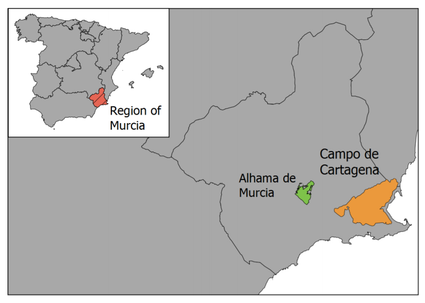
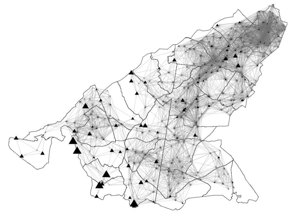
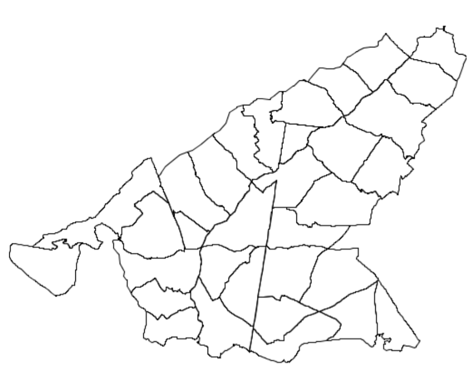
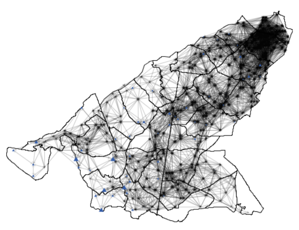
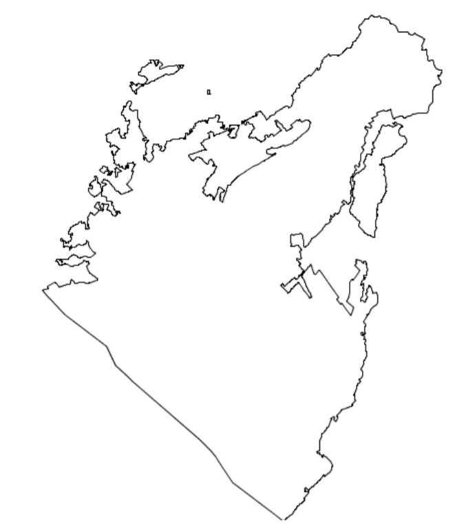
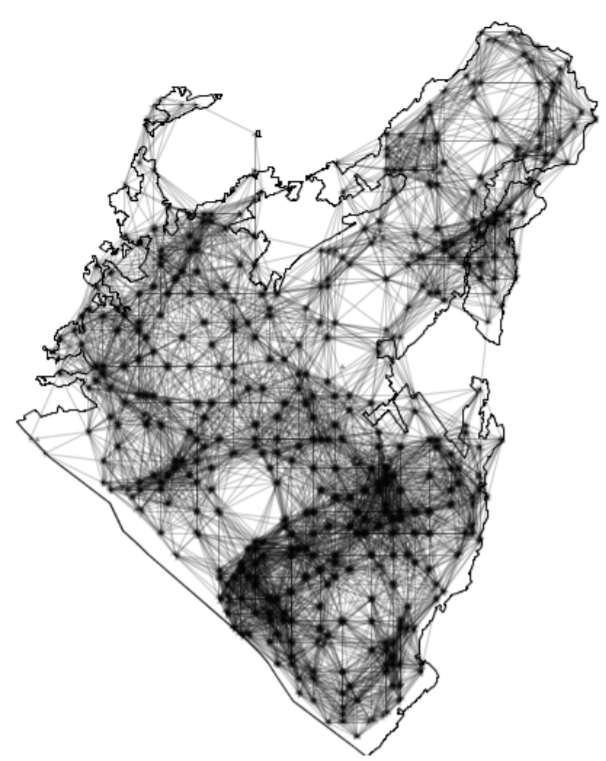
We use historical data from two Spanish irrigation communities: Alhama de Murcia and Campo de Cartagena. Both are located in the Segura river basin in SE Spain (Figure 3). In this region, water scarcity is severe and the average annual precipitation is low (approximately 300 mm/year). Thus, ICs receive surface water transfers from the Tajo river and farmers often draw from groundwater resources. Climatological conditions (i.e. evapotranspiration and precipitation) are regional normal values during 1981–2010 and are assumed constant over time. Crop variables (i.e. crop coefficients, yields, and prices) are set using national sources (MAPAMA 2017 ; Region of Murcia 2017; Regional Statistics Center of Murcia 2017; MAPAMA 2017b). Following experts’ opinions, individual modernisation is assumed to cost 3,500 eur/ha, to be paid in a 5-year time frame with a 2.5% interest rate. Global efficiency of the irrigation system (taking into account distribution and application) is set as 40 % and 75 % for traditional and modernised systems, respectively. Finally, social network maximum distance is 4 km (see Figure 4 as an example of spatial setup).
With regards to the actual modernisation process of the community as a whole, there is reliable data for both communities. The data set of the two communities is not complete, fortunately they mostly complement each other. Thus, given the similarities of the two ICs, we were able to model the variables of each stage drawing mainly on data from one community. Validating social processes of empirically-grounded models is difficult and has to cope with many uncertainties (Parker et al. 2003). We have stuck to replicative validation, comparing the simulation results with the real observations.
Stage 1: Collective modernisation
This stage is modelled mostly with data from Alhama de Murcia. This community has 5,906 hectares and 2,317 members. It started to operate in 1979 with a nominal allocation of 10,372,000 m3/year, although since then, it has received only up to 50%. In 1981, its General Assembly decided not to participate in the modernisation plan of the region. Nonetheless, it decided to modernise in 2000. Predominant crops in the area were citrus, grape, and other fruit trees and vegetables.
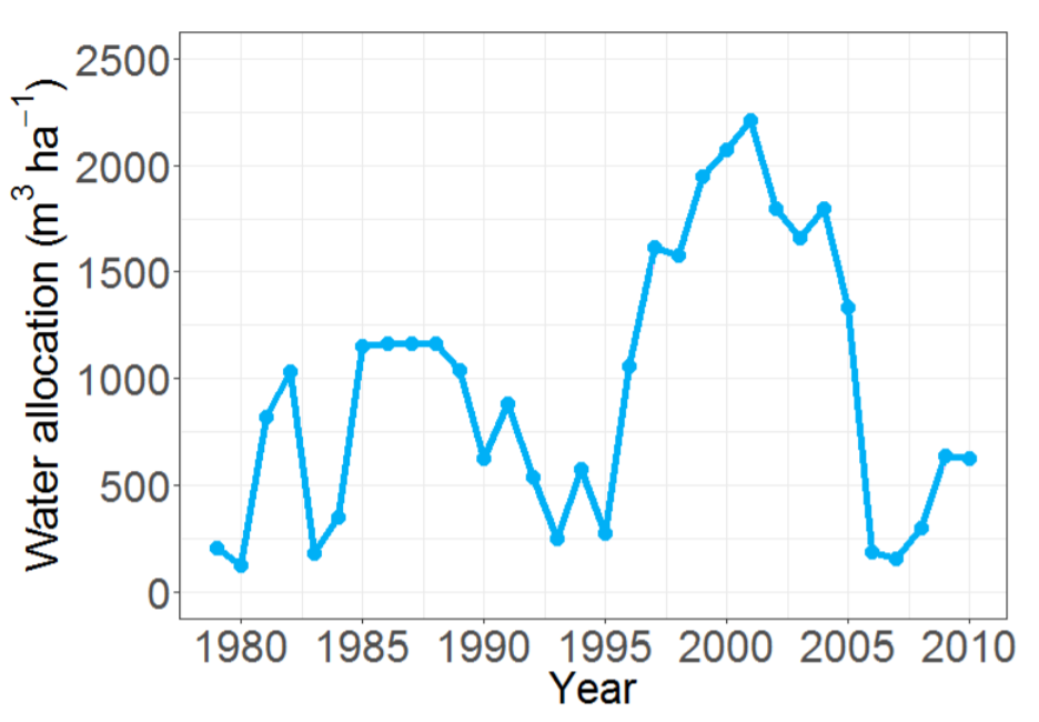
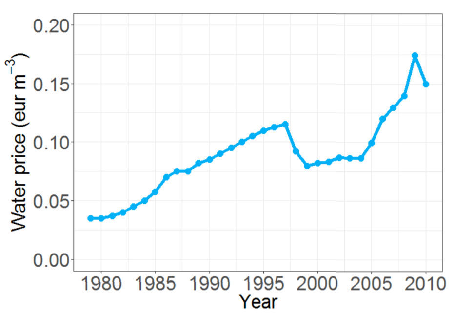
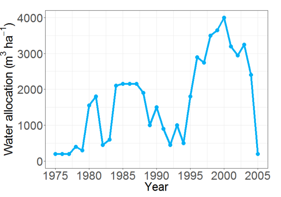
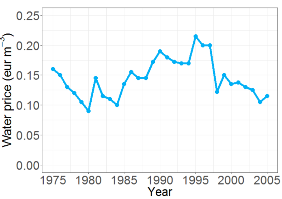
In order to simulate the collective disposition we used data from 1979 to 2010. Water allocations are published (Alhama de Murcia IC 2016), as well as water prices (SCRATS 2017). Crop options are a representative crop type in the aforementioned generic groups. Water fees are supposed to be 50 and 150 eur/ha/year, for traditional and modernised infrastructure, respectively. According to experts, collective modernisation costs are approximately 6,500 eur/ha with a payback period of 75 years. We used data from a nearby community (namely Campo de Cartagena) to define the individuals’ attributes. In this stage, the risk-aversion parameter \(\gamma_{S1}\) in Equation 6 is set empirically to 0.5 to fit observations, as done for Stage 2 (see Section 5.6). Simulations involved 440 agents and 300 runs for each experiment.
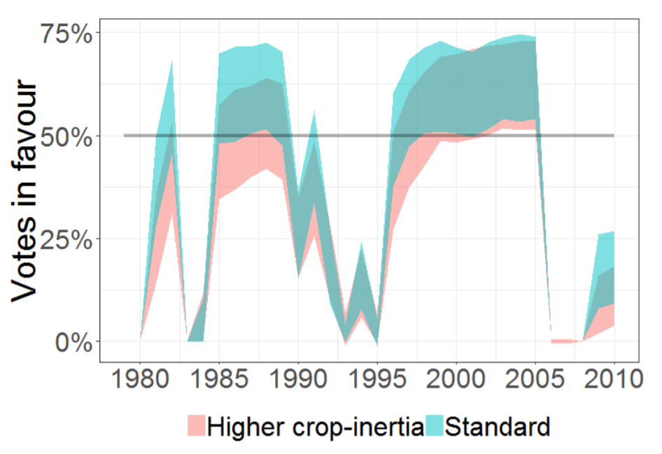
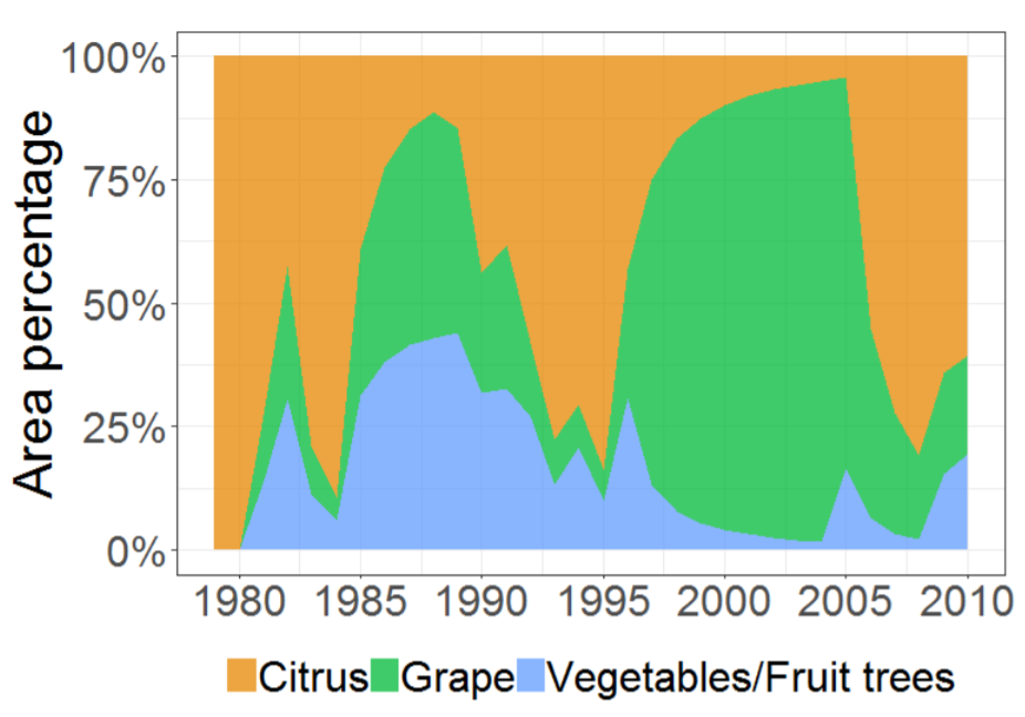
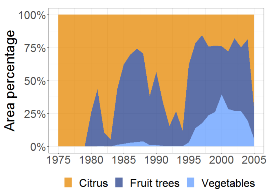
Results indicate an increase of votes in 1985-1990 and in 1995–2005 —slightly higher— (Figure 7). Figures 5 and Figure 6 show that they correspond with larger allocations and lower water prices, which enable new crop options that lead to added-value crops (Figure 8). Crop-inertia plays a key role because it favours a change to crops with higher marginal water value (Figure 7). During the 1985–1990 period, increased water supply leads to a mixture of two crops (Figure 8): one with a higher water marginal value and lower water requirement (vegetables) and another with a lower water marginal value but larger value and larger water requirements as well (grape). In this period, most farmers that switch crops in the high-crop inertia scenario, grow grapes because they have larger water supplies. In the low inertia scenario, more farmers switch crops, including farmers with lower water supplies that allow them to move only to lower value crops (they switch to vegetables but cannot produce grapes). In the 1995–2005 period, inertia is less relevant because, due to the increased availability of water, producing grapes is feasible for almost all farmers.
Stage 2: Individual modernisation
The second stage of the model is tested using data from Campo de Cartagena. It comprises 37,433 hectares and their predominant crops were vegetables, citrus, and fruit trees. Alcón (2007) collected data to build equation-based models of innovation diffusion for the period of 1975–2005. In that work, 360 farmers out of 3,237 were thoroughly characterised (e.g. age, farm area, support-supply, crop-inertia), and the water-related variables such as water allocations and water prices were given in detail[2]. In the absence of precise field data, we chose representative crops in the region for the three predominant types (vegetables, citrus, and fruit trees). As suggested before, risk aversion in this stage is larger because farmers are now committing their own money. Thus, the risk-aversion parameter \(\gamma_{S2}\) in Equation 6 is larger than the corresponding \(\gamma_{S1}\) in stage 1, namely, 1.085. The risk aversion when imitating \(\alpha_{t0}\) is 1.970 with a reduction \(\psi\) of 2% every year. These are equal for all farmers. In order to calibrate these parameters we tested different values for the risk-aversion parameters against the actual adoption curve (see Figures 11 and 12 and associated discussion starting in Section 5.6).
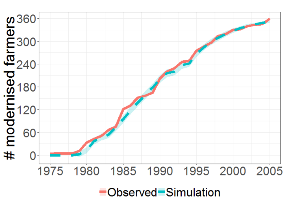
Adoption is triggered when innovators change crops and after that, the model shows that it spreads by imitation, regardless of crop patterns (Figure 9).The adoption curve that results from the simulation resembles the typical logistic function, as expected, and fits the actual curve (Figure 10).
Discussion
Simulations show reasonable correspondences with the studied cases in Spain. Significant increases in collective modernisation disposition are produced when farmers can leap to higher-value crops that have a greater water demand. These results are consistent with others like (López-Gunn et al. 2012b; Pfeiffer & Lin 2014).
The model is validated with real data. We had no information on individual farmers’ behaviour and social interactions beyond descriptive expert knowledge and agent attributes (e.g. farm area) but we had highly aggregated IC data (e.g. the adoption curve). We compared the results, which emerged from simulated individuals’ behaviour and social influence models, and found that they matched.
Our model identifies when favourable conditions appear. In other words, what is relevant is the evolution of the collective disposition and its local maxima. Although we have calibrated the model to reflect credible voting results, additional empirical data about agents’ resolutions is likely to improve calibration.
It can be deduced from the model that when water availability is too high, farmers do not perceive modernisation as advantageous, since their water demand would be completely satisfied and costs will increase unnecessarily (see Section Modernisation? in Appendix A). In other words, if farmers have as much water as they need to grow the highest water-demand crop —despite the water losses of the traditional system—, ‘modernisation’ is not attractive at all because it does not produce any extra profit. Although water losses are lower because of the innovation, they already have the volume they need for the chosen crop. In this case, “modernisation” does not lead to anything but higher costs.
Likewise, if water availability is low due to short allocations, farmers will not modernise since production increases do not compensate the costs or they cannot leap to higher-water-demand crops. Furthermore, uncertainty, and not only availability, affects decision-making (Alcón et al. 2014). This uncertainty could arise from environmental variables (rainfall resources and extreme weather events) or institutional reliability (whether the river basin authority or community can ensure the entire water allocation and water prices). We have not modelled uncertainty explicitly in our model beyond the risk-aversion and the imitation risk-aversion parameters.
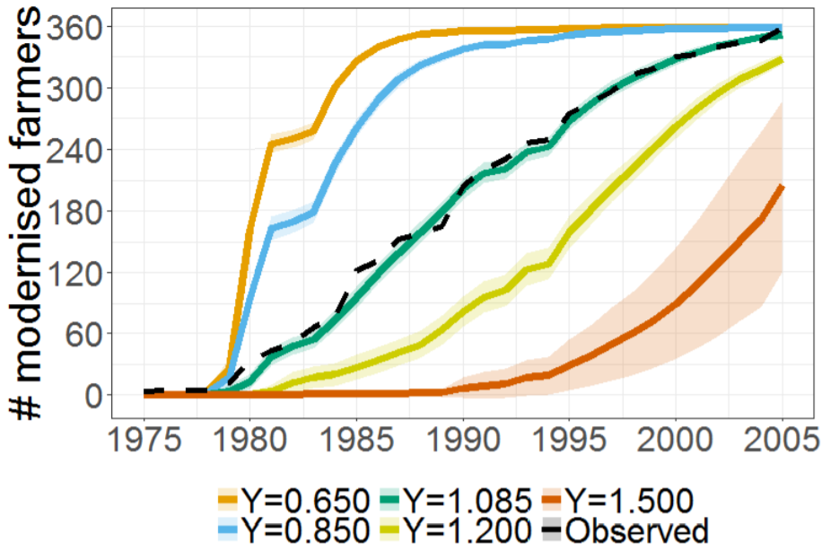
Varying risk-aversion supports intuitive results: the greater the risk aversion, the lower the adoption rate. Figure 11 shows that a risk-aversion \(\gamma_{S2}>1\), (i.e. status quo weighs more than future expectations) entails delayed adoption curves. Lower values for the parameter lead to a significant number of adoptions at the beginning, that are delayed by a period of low water allocations (Figure 5)—since greater water availability due to modernisation does not result in higher profits—, and then recover to slowly enter in a stationary phase. Notice that the “exponential growth” in the adoption curve is still notable for \(\gamma_{S2}>1\), which reflects that the delaying factor is presumably the lack of early adopters that spread the innovation (who decide to adopt at the end of the period, when highest water allocations are provided) —which also explains the deviation in simulation results. This exercise reveals the considerable sensitivity of the parameter: for instance, valuing the status quo only 0.85 in comparison to the expectation (see Equation 6) leads to a quite different adoption curve.
Similarly, imitation risk-aversion \(\alpha_{t0}\) shows higher sensitivity when \(\alpha_{t0}<2\) (Figure 12). For greater values (\(\alpha_{t0}>2\)), effects are reduced with respect to the base line, which may reveal that imitation, despite occurring, is infrequent. In other words, as the imitation risk-aversion parameter increases, the “social effects” are practically suppressed.

Since the shape of the estimated adoption curves follows a logistic curve as expected, our choice of the values for risk aversion parameters is guided by the extremes of the actual adoption curves. Better grounds for fixing risk aversion parameters should come from field data from these and other communities. However, as incidental support to our approach, notice that the shape of the estimated curves not only fits nicely the rest of the interval but also reproduce the “bumps” of the actual curves. Thus, for example, our model estimates that adoption is almost absent in periods of low water allocation (1981–1984 and 1987–1994 in Figure 5), a phenomenon that is also visible in the real adoption curve and is easily observable in Figure 12).
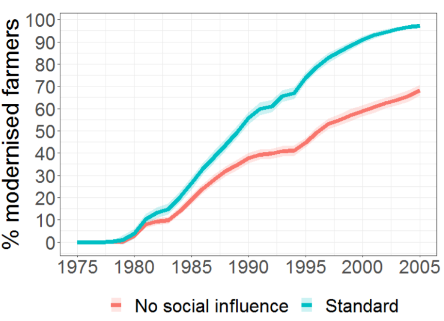
Modernisation affects the efficiency of the irrigation infrastructure, but it requires a proper management as well (Coward 1991; Naranjo Chicharro 2010). Although these factors were not introduced in the model, it is expected that an efficient management would accelerate adoption and diffusion because of two reasons: (i) a poor management implies that not all potential benefits are entirely exploited, making modernisation less attractive to farmers; and (ii) untrained farmers are less successful, hence less likely to be imitated by other farmers. Since in our model imitators only perceive the consequences of the modernisation —i.e. revenue and not the new crop options— they fail to assess the total benefits. According to the simulations, this social influence is relevant for the second stage: without it, only 70 % of the farmers eventually adopt (Figure 13). This also suggests that an appeal to profit-driven motivations is more likely to be successful when it is addressed to opinion leaders in those communities that are market-driven, able to adopt new crops and threatened with water limitations.
Experts have proposed other conditions for modernisation that could be approached as extensions of the current model. Two are noteworthy: (1) Ortega (2015) reported that some farmers were deceived: while modernisation was offered for free or strongly subsidised, in practice farmers had to pay for it, which hindered financial sustainability. In our model, it means that farmers used optimistic values which led to collective modernisation that would not have happened if they had not been misled. (2) In our model, collective decision is approached as a bottom-up aggregation of individual dispositions, a reasonable assumption for communities in which the social structure is horizontal. However, in some communities there is a small number of promoters of modernisation who try to influence other members to vote in its favour: politicians or community presidents promote modernisation in order to gain recognition or increase power (see Sanchis-Ibor et al. 2017). In this case, only a few agents would decide (Equations 3–6), and the diffusion model (Equation 7 and social network building) would consider other social characteristics to weigh the influence.
Edmonds 2005 pointed out the problems of representing opinions as numerical measurements and indicated the concerns when using such approach in causal mechanisms of the simulation model. We are aware that we make a strong assumption representing the disposition to modernise by a simple numerical score, and use it in particular social influence functions. Modernisation may be motivated (or rejected) by combinations of other values besides economic profit: for instance, comfort, time savings due to automatisation, sense of progress, etc. In other words, decisions about modernisation arise, presumably, from a more complex model of rationality (which not only takes economic profit into consideration). This points for further research in how to work with values in computational models.
For these reasons, and although the results are encouraging, more field research is needed to better ground some assumptions in the model —for example, non-economic values (e.g. tradition, power, etc.), risk-aversion and crop-inertia parameters, social network generation— to apply it in communities whose socio-hydrological characteristics are different from the ones whose data we used. We think that fieldwork should be done to further explore the farmers’ values and their understandings —as pointed out by Huber et al. (2008) —, since this will shape how the behaviour of the artificial farmer agents is modelled (see also Hitlin & Piliavin 2014; Schwartz 2012).
Finally, it is convenient to remark that modernisation has been questioned from a perspective focused on environment conservation perspective (López-Gunn et al. 2012a, López-Gunn et al. 2012b; Perry et al. 2009). It has been suggested that modernisation leads to farming intensification (e.g. extension of the farming area, double-cropping, or the adoption of crops with higher water demand), eventually increasing the use of water resources. One of the reasons, for instance, is that farmers are forced to intensify their production in order to compensate higher energy costs —phenomena that is aggravated because energy prices are continuously rising, while prices in agricultural markets follow a downward trend (López-Gunn et al. 2012a).
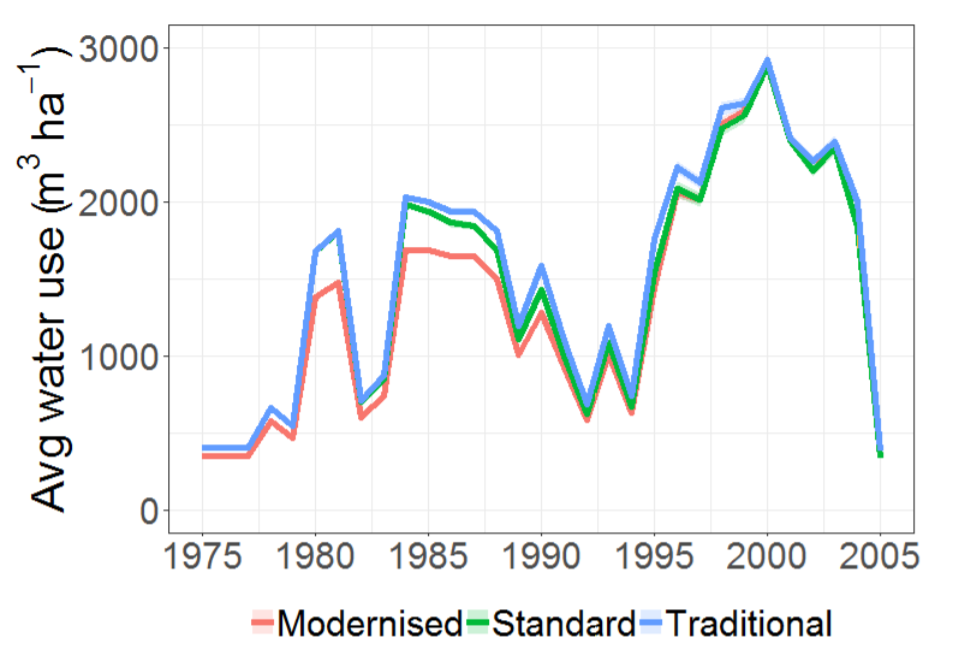
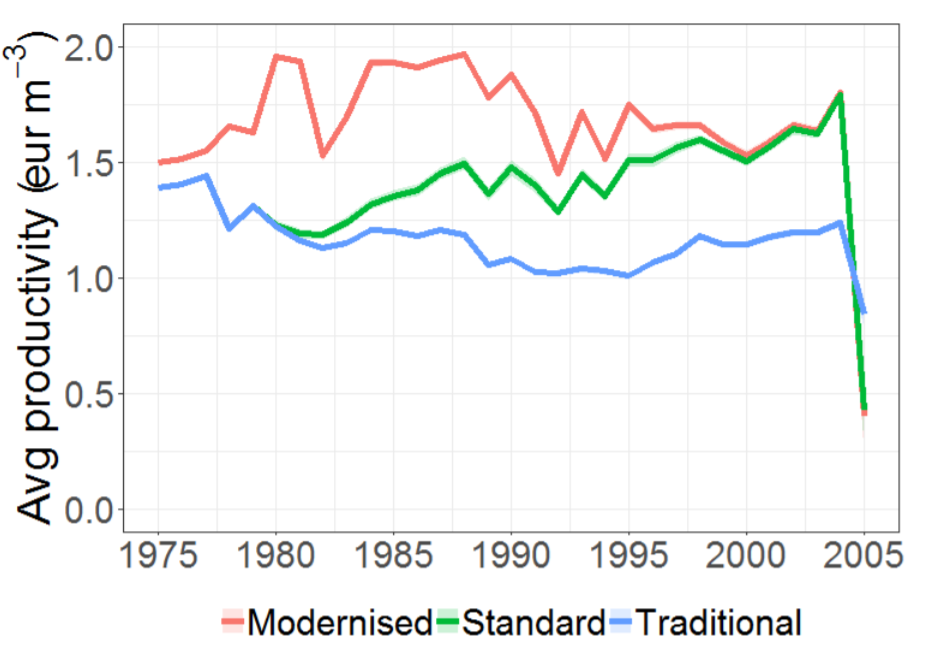
Although farming intensification in the model can only be produced by the adoption of crops with higher water-demand, the aforementioned phenomena is reflected in the simulations. Three scenarios have been simulated for Campo de Cartagena: (i) a standard scenario, where farmers adopt progressively (as they do in Figure 10); (ii) a traditional scenario, in which individual farmers keep using traditional methods and do not adopt modern technology at any time; and (iii) a modernised scenario, in which farmers adopt the technology from the start of the simulation. As Figure 14 shows, the three scenarios are almost identical and modernisation results in low water savings. What modernisation actually promotes is water productivity (Figure 15) —which is, in fact, more sensitive to water allocation changes[3]. This indicates one of the trade-offs that public policy has to deal with, and different understandings of what ‘efficiency’ is in this particular domain (see also Perry et al. 2009). Therefore, it has been suggested that additional policy instruments are necessary if environment conservation (namely, water savings) is pursued, such as updating water allocations and water tariffs (see López-Gunn et al. 2012b).
Closing Remarks
We developed an agent-based model to explain modernisation of the irrigation system in farmer communities. Modernisation is modelled as a contingent innovation-diffusion process: a first stage where the community establishes a collective agreement to modernise —based on individuals’ dispositions— followed by an individual adoption decision. The model was built using historical data (1975–2010) from two Spanish irrigation communities where water is scarce and efficient irrigation (resulting in higher water availability) enables more profitable crop types that are commercially consolidated.
The model is predictive for modernisation under such particular conditions. It can be used by policy makers to foster modernisation in similar contexts, to incentivise or subsidise the emergence of the propitious conditions, or to either dismiss modernisation or identify (alternative) non-profit driven motivations.
Although results are promising, we recognise that this model has some limitations. Conceptually speaking, bounded rationality of farmers should be further improved using more fieldwork. Also, some of the assumptions made to simplify the model or due to lack of data could be improved in further versions (e.g. there is no lag between crop-decision and crop-production, which may be inappropriate for tree-type crops; constant and current crop prices; etc.). Moreover, input from experts and available data may have driven the modelling process towards some consolidated worldviews about farmer communities.
These results are but a modest first step into a larger project of using agent-based modelling in policy-making and the role of values as the main research motivation (Perello-Moragues & Noriega In Press). The immediate next step is to bring non-economic values in the individual decision-process. Field studies like (Alcón 2007) have pointed out that variables like age, education, or time-savings affect individual dispositions. There are also communities that rejected modernisation subsides on, for instance, grounds of preservation of lifestyle and landscape (Alcón, personal communication), while others adopted due to misleading agents (Ortega 2015; Sanchis-Ibor et al. 2017).
Despite the fact that this model puts emphasis on water economy, the model could be extended to consider a broader approach for policy-making, namely taking the Food-Energy-Water nexus into account. As (Cai et al. 2018) pointed out, ABM is a promising modelling approach to consider that perspective. We think that the case presented in this paper is particularly interesting, as it combines agricultural economy, water governance, and the use of energy-intensive technologies (López-Gunn et al. 2012a, López-Gunn et al. 2012b).
Finally, we believe that this paper makes three contributions for the ABS community: (a) identifies a problem domain that involves a rich repertoire of challenges (value-driven decision-making; collective agreement, policy design, negotiation, etc.), (b) constitutes a real practical application based on real data, and (c) provides a non-trivial illustration of how policy-makers and businesses may adopt ABM for their interests.
Acknowledgements
Francisco Alcón gave us valuable criticism. Experts from Aqualia and Agbar-Suez provided input on modernisation processes and facilitated field visits. The first author is supported with the industrial doctoral grant 2016DI043 of the Catalan Secretariat for Universities and Research (AGAUR), sponsored by FCC AQUALIA SA, IIIA-CSIC, and Universitat Autònoma de Barcelona (UAB). This research has been also supported by the CIMBVAL project (Spanish government, project # TIN2017-89758-R).Notes
- To initialise the simulation, the age of farmers —attribute (vi)— is set with real data, but it also changes with time.
- F. Alcón gave us access to unpublished data from (Alcón 2007) that we used to set these parameters.
- Water productivity is calculated as the revenue (Equation 3) divided by the gross water volume used from the water allocation (that is, before water losses). The gross water volume relative to the area (Figure 14) may not reach the level of the water allocation (Figure 18 in Appendix B) because (i) the allocation is distributed equally among the whole crop season, but (ii) the crop requirements are different for each month.
- http://www.aemet.es/es/serviciosclimaticos/datosclimatologicos/valoresclimatologicos?l=7031&k=mur
- https://www.cralhama.org/el-trasvase-tajo-segura-y-los-regadios.
- http://www.scrats.es/tarifas-vigentes.html.
- https://www.ine.es/jaxi/Tabla.htm?path=/t01/p042/a2009/prov00/l0/&file=1101.px&L=0.
- https://www.cralhama.org/distribucion-de-cultivos-propiedad-y-sistema-de-riego/.
- https://www.crcc.es/informacion-general/documentos-y-planos/.
- https://www.cralhama.org/zona-regable/.
- https://www.chsegura.es/chs/cuenca/resumendedatosbasicos/cartografia/descargas/.
Appendix
A: Submodels
This appendix complements Section 3.
For the sake of simplicity we omit subindex t (time-step) in all formulas, where time-step is one year.
Water availability
Farmers estimate the expected volume of water available to irrigate for that year. This volume of water resources is given by:
- The water allocation of the community, \(W_{allocation}\), for that particular year.
- The supply support \(S_{i}\), which represents the share of the supplied water resources withdrawn from alternative sources like private wells. Therefore, this volume \(W_{support,i}\) is calculated (Equation 12):
- The effective precipitation, \(P_{e}\), that is the fraction of precipitation that can be potentially used by crops, considering that there is a fraction that leaves the system (as runoff, for instance). It is assumed that only 75% of the total precipitation \(P\) is effective precipitation.
- The irrigation infrastructure (constituted by the collective distribution and individual application systems), that determines the fraction of water that leaves the system (as leakage or evaporation) and cannot be used in crop evapotranspiration (Table 1).
| $$ \small{ W_{support,i} := \frac{S_{i} \cdot W_{allocation}}{1-S_{i}} }$$ | (12) |
The irrigation infrastructure determines the amount of water that is actually applied to the crop. A fraction of the total volume of water leaves the system due to system losses (i.e. leakage or evaporation). Thus, considering the efficiency of water distribution \(\mu_{d}\) and the efficiency of water application \(\mu_{a,i}\) (that depends on the farmer), the water allocation \(W_{allocation}\) is reduced to (Equation 13):
| $$\small{ W'_{allocation,i} := W_{allocation} \cdot \mu_{d} \cdot \mu_{a,i} }$$ | (13) |
Likewise, the support is reduced to (Equation 14):
| $$\small{ W'_{support,i} := W_{support,i} \cdot \mu_{a,i} }$$ | (14) |
| System | Collective, Distribution (\(\mu_{d}\)) | Individual, Application (\(\mu_{a,i}\)) |
| Traditional | 0.75 | 0.55 |
| Modernised | 0.85 | 0.90 |
Water partition
It is assumed that the water allocation and supply support is distributed uniformly along the season —those months in which the crop requires to be irrigated, that is, \(K_{c,j} \neq 0\) for month j—, although we recognise that other considerations could be done at this point (for instance, that the volume is distributed equally along all the year regardless of the crop requirements).
Considering that the season comprises \(m\) months (i.e. the number of months with \(K_{c} \neq 0\)) (see Table 3 in Appendix B), then, the available water for each is (Equations 15 and 16):
| $$\small{ W'_{allocation,i,m} := \frac{W'_{allocation,i}}{m} }$$ | (15) |
| $$\small{ W'_{support,i,m} := \frac{W'_{support,i}}{m} }$$ | (16) |
Water Irrigation
This procedure is done along the year for all the months. If the crop requires to be irrigated in month j (\(K_{c,j} \neq 0\)), then the farmer i uses all the water available for that month (Equations 17):
| $$\small{ W_{i,j} := W'_{allocation,i,m} + W'_{support,i,m} + P_{e,j} }$$ | (17) |
The water requirement for crop c is calculated as the reference evapotranspiration \(ET_{0,j}\) (which depends on climatological variables, such as temperature) multiplied by the crop coefficient \(K_{c,j}\) (Allen et al. 1998) (Equation 18):
| $$\small{ ET_{c,j} = K_{c,j} \cdot ET_{0,j} }$$ | (18) |
Then, the available water is compared to the required water to determine the volume of irrigation water I. Two cases are identified:
- Case (a): \(W_{i,j} \geq ET_{c,j}\), which means that there is enough water to satisfy the crop water requirement. In this case, the farmer uses only the required volume (not all the available water) (Equation 19):
- Case (b): \(W_{i,j} < ET_{c,j}\), which means that the crop is under water deficit conditions. In this case, the farmer uses all the water that is available, although it does not satisfy the water requirement (Equation 20):
| $$\small{ I_{j} := ET_{c,j} }$$ | (19) |
| $$\small{ I_{j} := W_{i,j} }$$ | (20) |
Notice that water used to irrigate has different sources (see Equation 17). Accordingly, the farmer uses the different sources following a policy of minimising the cost of water. With this in mind, the first source to be used is precipitation, then the community allocation (Equation 15), and finally the individual sources (Equation 16), which are assumed to be more expensive than the other sources —mainly because they are groundwater resources and also not all the agents have access to them.
Crop yield estimation
Crop yield is estimated using the following relationship (Steduto et al. 2012) (Equation 21):
| $$\small{ \bigg[ 1 - \frac{Y_{a}}{Y_{max}} \bigg] = K_{y} \bigg[ 1 - \frac{ET_{a}}{ET_{max}} \bigg] }$$ | (21) |
In the model, crop yield is addressed as follows:
- First, the evapotranspiration ratio \(ET_{a}/ET_{max}\) is calculated for each month j. Using the variables as named in the previous submodels, it is computed as (Equation 22):
- Second, the yield ratio \(Y_{a}/Y_{max}\) is obtained following Equation 21 considering the crop yield response factor \(K_{y,c}\) (Equation 23):
$$\small{ \lambda_{j} := \bigg( \frac{Y_{a}}{Y_{max}} \bigg)_{j} = 1 - K_{y,c}(1-\xi_{j}) }$$ (23) - Third, the average of the yield ratio is estimated for the whole crop season (that comprises m months) (Equation 24):
| $$\small{ \xi_{j} := \frac{I_{j}}{ET_{c,j}} }$$ | (22) |
| $$\small{ \bar{\lambda} = \frac{1}{m}\sum_{j}^{m}\lambda_{j} }$$ | (24) |
Accordingly,
- In Case (a), crop requirements are satisfied. Each additional water unit does not increase the crop yield, since the maximum production is reached. If farmers are considering to modernise their systems, the investment is less attractive, since the yield for that crop c does not change with more water.
- In Case (b), the crop is under water deficit conditions. Each additional water unit increases the crop yield. Due to this fact, modernisation is more valuable, since it can lead to a greater production with the same water allocation (because less water is lost by leaks and evaporation).
Production
In this procedure, the economic output of farmers is computed.
First, the crop production is estimated (in tonnes), taking into account the actual crop yield (Equation 24) and the characteristics of the crop (Table 3 in Appendix B) (Equation 25). It can be used to calculate the income (in euros) (Equation 26).
| $$\small{ Production_{i,c} := \bar{\lambda} \cdot Y_{max,c} \cdot Area_{i} }$$ | (25) |
| $$\small{ Income_{i,c} := Production_{i,c} \cdot Price_{c} }$$ | (26) |
Second, the farmer has to cover the costs of the activity. There are two main costs: (i) on the one hand, there are individual costs that are associated to the water application system and to farming as a productive activity; (ii) on the other hand, there are collective costs that are associated to the administration of the community and its collective water distribution infrastructure (i.e. investment, operation, maintenance, etc.). These costs are covered by water fees, which are established by the irrigation community, that are paid individually by all the farmers of the community. These fees are implemented by means of different water tariff schemes:
- A tariff scheme whose pricing is proportional to the farmers’ irrigated area. This scheme is used by traditional communities (i.e. non-modernised).
- A tariff scheme whose pricing is a binary cost-allocation scheme: a fixed fee that is proportional to the irrigated area, plus a variable fee proportional to the volume of water used. This scheme is used by those communities that have modernised their collective distribution infrastructure. Some communities may base their water fees entirely on the variable term.
With this in mind, a farmer i has to consider multiple costs:
- Costs of water \(C_{w,i}\) (Equation 27 for traditional communities and Equation 28 for modernised communities):
- Costs of operation and maintenance of the farm \(C_{O\&M,i}\) (Equation 29):
- Costs of private supply \(C_{p,i}\) (Equation 30):
- Costs of amortisation \(C_{a,i}\) (to replace the individual application system). The total cost is calculated as (Equation 31):
| $$\small{ C_{w,i} := fee_{w,trad} \cdot Area_{i} }$$ | (27) |
| $$\small{ C_{w,i} := fee_{w,mod} \cdot Area_{i} + U_{w} \cdot Area_{i} \cdot \frac{I_{allocation,i}}{\mu_{a,i}} }$$ | (28) |
| $$\small{ C_{O\&M,i} := U_{O\&M} \cdot Area_{i} }$$ | (29) |
| $$\small{ C_{p,i} := U_{p} \cdot Area_{i} \cdot \frac{I_{support,i}}{\mu_{a,i}} }$$ | (30) |
| $$\small{ C_{A} := Inv_{i} + \sum^{T}_{t=1} Inv_{i} \cdot (1-\frac{t}{T}) \cdot r }$$ | (31) |
With this in mind, and considering equal payments along the lifespan, the amortisation cost is (Equation 32):
| $$\small{ C_{a,i} := \frac{C_{A}}{T} }$$ | (32) |
Then, the total costs for a farmer i are calculated as (Equation 33):
| $$\small{ Costs_{i} := C_{w,i} + C_{O\&M,i} + C_{p,i} + C_{a,i} }$$ | (33) |
Finally, the revenue is computed as the difference between the income (see Equation 26) and the costs (see Equation 33) (Equation 34):
| $$\small{ Revenue_{i} := Income_{i,c} - Costs_{i} }$$ | (34) |
Crop choice
In this procedure, farmers choose the crop type for their farms in order to maximise their revenue. Nonetheless, they may be reluctant to change crops in spite of potential profitability due to risk aversion, specialisation, comfort, etc. All these factors are reflected by crop-inertia\(\phi\). It is implemented as (Equation 35):
| $$\small{ P_{i}[change \, crop] = 1 - \phi_{i} }$$ | (35) |
If this event is unsuccessful, the farmer will grow the same crop as the previous year. On the contrary, if the event is successful, the farmer will explore the multiple crop options (see, for instance, Table 3 in Appendix B). This consideration may be seen, somehow, as path-dependence on farmers’ decision-making (as their decision depends, to some degree on their current land-use).
Taking into account the actual irrigation system (i.e. collective and individual), and using the previous submodels (namely, water availability, water partition, water irrigation, crop yield estimation and production submodels), it is possible to estimate the actual revenue for each crop option. The chosen crop is the crop option that maximises their revenue.
Actual production
Assuming that a farmer has chosen a crop, and using the previous submodels (namely, water availability, water partition, water irrigation, crop yield estimation, production, and crop choice submodels), the actual revenue of the farmer can be computed, which determines the variations of their capital. The farmer then memorises this revenue as past revenue (Equation 3).
Modernisation?
Note: as this submodel has been explained in Section 3, this subsection will only provide some further details, and will not reproduce again the entire submodel.
In Stage 1, farmers evaluate how modernisation will impact on their economy. To do so, they compare the results between the current irrigation system (that is, traditional collective and individual systems) against a modernised irrigation system (both collective and individual systems). Generally, modernisation may increase the water availability, which can open new crop options that lead to greater income. However, costs also increase, mainly due to the investment that has to be made to install such systems.
In specific terms, farmer compare the revenue (Equation 34) that is produced using the current traditional system (Equation 3) with the one that is produced using a modernised system. Namely, an expectation is generated (Equation 4) making use of the previous submodels (i.e. water availability, water partition, water irrigation, crop yield estimation and production submodels) assuming that a modernised irrigation system is being used. This expectation is then compared to the past revenue (Equation 5).
Notice that the individual modernisation costs (Equations 31 and 32) may take into account different payback periods (for instance, in the simulation, farmers evaluate modernisation as they would have to pay the investment in 5 years).
In Stage 2, farmers use the same process of decision-making, but the conditions have changed slightly (the risk-aversion parameter, the collective infrastructure, and the social influence process) (see Section 3). Once the community decides to modernise their collective infrastructure (that is, the community goes from the Stage 1 to the Stage 2), farmers are not willing to modernise their individual application systems any more, and have to make the decision again with the new conditions.
Assembly
In Stage 1, the community holds an assembly to pass the proposal of modernising the collective infrastructure. The system is based on direct voting, in which each member of the community has a specific number of votes proportional to the area of its farm.
The community will commit to modernise only when more than half of the votes are for modernising. In practice, that means that more than 51% of the area of the community is subject to be modernised, as the farmers who own that extension are willing to modernise. Besides, a farmer cannot have 51% of the votes by itself (that is, at least two farmers have to vote in favour).
For the sake of simplicity, only farmers who are active and willing to modernise vote in favour.
Activity?
Each year, farmers decide whether to quit or not depending on the revenue from the previous seasons and the capital they have.
If the actual revenue is negative (that is, the farmer is losing money), the farmer is more prone to quit: facing three consecutive years of negative results will force the farmer to become inactive and leave their farm unproductive. Likewise, if the individual capital drops to below than 0 eur, then the farmer will become inactive too.
Population evolution
Each year, farmers’ age increases by one. This can lead them to reach the retirement age and trigger a generational replacement.
When farmers reach the retirement age, they can either (a1) be replaced by a new farmer or (b1) retire and leave the farm unproductive (for instance, because they do not manage to find a successor). In this model, the retirement age has been set to 80 years old; the probability of event (b1) is 0.60; and the probability of event (a1) is the complementary.
In case of event (a1), the new farmer is between 18 and 45 years old, and not willing to modernise (that is, the decision process has to be made again). Notice that, if the individual system of the farm has been already modernised, the new farmer has no decision to make in that matter.
Moreover, inactive farmers can (a2) remain inactive, (b2) become active again, or (c2) transfer the land to a new farmer.
We assume that the probability of event (a2) is 0.80, and the probability of both events (b2) and (c2) is the complementary. In this latter case, the probability of event (c2) is 0.05. As before, the new farmer is between 18 and 45 years old, and not willing to modernise (that is, newcomers have to make the decision process again).
B: Input data
A summary of the input data for the simulations can be found inTable 2.
Crop options and characteristics
According to Alcón (2007), in Campo de Cartagena, predominant crops are vegetables, citrus, and fruit trees —at that time, they accounted for 51%, 35% and 8%, respectively. In Alhama de Murcia, predominant crops included citrus (45%), vineyards (35 %), and vegetables and fruit trees (20 %) in 2018 (Alhama de Murcia IC 2018).
Table 3 shows the crop options that have been considered in the simulation. Crop characteristics (i.e. evapotranspiration factors, maximum yield, prices, and yield response to water stress) were collected from diverse sources (Steduto et al. 2012; Allen et al. 1998; MAPAMA 2017; Region of Murcia 2017; Regional Statistics Center of Murcia 2017; MAPAMA ND). In the absence of precise field data, we have chosen representative crops in the region for the predominant ones: namely, orange (Citrus), lettuce (Vegetable), peach (Fruit-tree), and lettuce + watermelon (Vegetable2). Grape is only available for Alhama de Murcia.
Climatological conditions
Climatological conditions (i.e. reference evapotranspiration \(ET_{0}\) and precipitation \(P\) ) are regional normal values per month during 1981–2010.[4] In the absence of precise historical meteorological data, they are assumed constant over time (that is, each year values are repeated).
| Variable | Input | Sources | |
| Crops | Crop factors \(K_{c}\) | See Table 3 | Allen et al. (1998); MAPAMA (ND) |
| Yield water response \(K_{Y}\) | See Table 3 | Steduto et al. (2012) | |
| Maximum yield \(Y_{max}\) | See Table 3 | MAPAMA (2017); Region of Murcia (2017); Regional Statistics Center of Murcia (2017) | |
| Crop prices \(Price_{c}\) | See Table 3 | MAPAMA (2017); Region of Murcia (2017); Regional Statistics Center of Murcia (2017) | |
| Climate | Effective precipitation \(P_{e}\) | See Table 4 | AEMET |
| Evapotranspiration \(ET_{0}\) | See Table 4 | AEMET | |
| Water economy | Water prices \(U_{w}\) | See Figures 17, 19 | Alcón (2007); SCRATS (2017); Alhama de Murcia IC (2016) |
| Water allocations \(W_{allocation}\) | See Figures 16, 18 | Alcón (2007); Alhama de Murcia IC (2016) | |
| Water fees \(fee_{w,trad}\) (Stage 1) | 50 eur/ha | Set by experts | |
| Water fees \(fee_{w,mod}\) (Stage 1) | 150 eur/ha | Set by experts | |
| Farmers | Age | See Table 5 | Alcón (2007), INE |
| Farm area \(Area_{i}\) | See Tables 6, 7 | Alcón (2007); Alhama de Murcia IC (2018) | |
| Supply-support \(S_{i}\) | See Tables 8, 9 | Alcón (2007) | |
| Crop-inertia \(\phi_{i}\) | See Tables 10, 11 | Alcón (2007) | |
| Risk aversion \(\gamma_{S1}\) (Stage 1) | 0.5 | Set by authors | |
| Risk aversion \(\gamma_{S2}\) (Stage 2) | 1.085 | Set by authors | |
| Imitation risk aversion \(\alpha_{t0}\) (Stage 2) | 1.970 | reduction \(\psi\) (Stage 2) | |
| Imitation risk aversion reduction \(\psi\) (Stage 2) | 2% | Set by authors | |
| Individual modernisation | Unitary cost \(U_{t}\) | 3,500 eur/ha | Set by experts |
| Interest rate \(r\) | 2.5% | Set by experts | |
| Payback period \(T\) | 5 years | Set by experts | |
| Crop | KC(–) | Ymax (T/ha) | KC (–) | Price (eur/T) | |||||||||||
| M1 | M2 | M3 | M4 | M5 | M6 | M7 | M8 | M9 | M10 | M11 | M12 | ||||
| Null | 0 | 0 | 0 | 0 | 0 | 0 | 0 | 0 | 0 | 0 | 0 | 0 | 0 | 0 | 0 |
| Citrus | 0.5 | 0.5 | 0.6 | 0.6 | 0.6 | 0.7 | 0.7 | 0.7 | 0.7 | 0.6 | 0.5 | 0.5 | 40 | 0.85 | 390 |
| Fruit-tree | 0 | 0.4 | 0.6 | 0.8 | 1.0 | 1.0 | 0.7 | 0.2 | 0 | 0 | 0 | 0 | 30 | 1.1 | 550 |
| Vegetable | 0.4 | 0 | 0 | 0 | 0 | 0 | 0 | 0 | 0 | 0.6 | 0.9 | 0.9 | 30 | 1.15 | 150 |
| Vegetable2 | 0.4 | 0 | 0.2 | 0.3 | 0.9 | 0.9 | 0.6 | 0 | 0 | 0.6 | 0.9 | 0.9 | 55 | 1.1 | 275 |
| Grape | 0 | 0 | 0 | 0.5 | 0.6 | 0.7 | 0.7 | 0.3 | 0 | 0 | 0 | 0 | 26 | 0.85 | 765 |
Effective precipitation (\(P_{e}\)) is the fraction of precipitation that can be potentially used by crops, considering that there is a fraction that leaves the system (as runoff, for instance). It is assumed that only 75% of the total precipitation is effective precipitation (although we recognise that more sophisticated models are available to estimate this fraction). These variables are usually given in millimetres or L/m2;; they have been converted to m3/ha to facilitate the operation with crop-related models.
Table 4 shows the climatological conditions —for each month of the year— that have been used in the simulation.
| M1 | M2 | M3 | M4 | M5 | M6 | M7 | M8 | M9 | M10 | M11 | M12 | |
| ET0 | 561 | 638 | 880 | 1153 | 1428 | 1740 | 1791 | 1625 | 1200 | 865 | 590 | 497 |
| Pe | 192 | 145 | 163 | 242 | 151 | 23 | 13 | 17 | 140 | 343 | 229 | 247 |
Water prices and water allocations
For Alhama de Murcia, water fees are supposed to be 50 eur/ha/year for the traditional collective infrastructure (see Equation 27). For the modernised collective infrastructure, water fees are supposed to be 150 eur/ha/year (fixed fee), to which the variable fee that depends on the volume used to irrigate and the water price has to be added (see Equation 28). Water allocation and water prices can be seen in Figures 16 and 17. This data was obtained from Alhama de Murcia IC (2016); SCRATS (2017).[5][6]
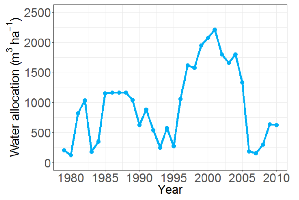
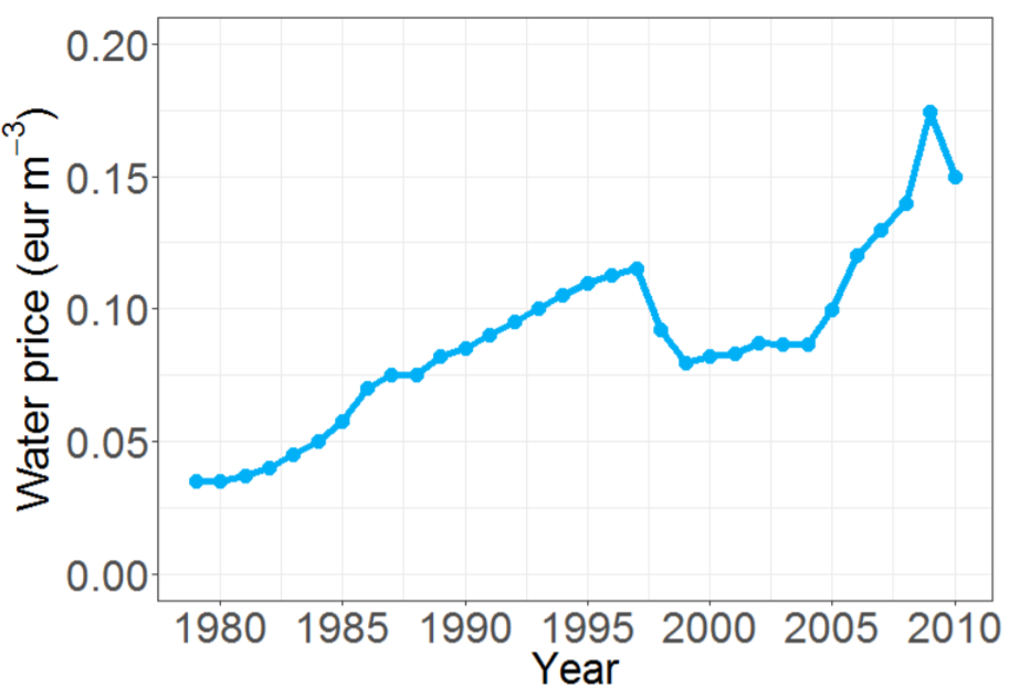
For Campode Cartagena, the tariff scheme is based entirely on the volumetric term (see Equation 28). Water allocation and water prices can be seen in Figures 18 and 19. This data was obtained from Alcón (2007). Notice that, for both communities water allocations follow a similar distribution, although Campo de Cartagena’s is almost twice as large.
Farmers characterisation
Alcón made available unpublished data from (Alcón 2007) that we used to characterise farmers in our simulation. Alcón conducted field surveys and collected data about farmers in Campo de Cartagena. We had access to individual agent’s data for variables such as age and farm area but, for privacy concerns, in this appendix we show only aggregated data.
In the absence of data for Alhama de Murcia, data from Alcón (2007) was used to characterise farmers in that community. For this purpose, the values for farmers variables were randomised using normal distributions whose mean and deviation were obtained from the sample of Campo de Cartagena.
Age
Table 5 shows the characterisation by age of farmers. In Campo de Cartagena, age was characterised according to Alcón (2007). In Alhama de Murcia, age was set following the statistical distribution from the Spanish agricultural census in 2009.[7] In this latter case, as only aggregated data was available, a random value in the range was generated following a uniform distribution.
| Age range | Alhama de Murcia proportion(%) | Campo de Cartagena proportion(%) |
| <25 | 0.3 | 0.3 |
| 25–34 | 4.5 | 12.5 |
| 35–44 | 13.6 | 28.7 |
| 45–54 | 22.3 | 19.8 |
| 54–64 | 26.3 | 22.8 |
| >65 | 33.0 | 15.9 |
Farm area
Table 6 shows the distribution of farmers by farm area in Campo de Cartagena, which was set according to Alcón (2007).
| Category | Proportion (%) |
| < 1 ha | 3.9 |
| 1–2 ha | 4.2 |
| 2–5 ha | 10.0 |
| 5–10 ha | 13.1 |
| 10–20 ha | 22.3 |
| 20–30 ha | 11.7 |
| 30–50 ha | 17.5 |
| 50–70 ha | 6.7 |
| 70–100 ha | 3.3 |
| ≥ 100 ha | 7.2 |
In Alhama de Murcia, field data was available, but it does not allow a precise characterisation of farmers (Alhama de Murcia IC 2018).[8] They provide the total number of farms, and their distribution by areas using broad ranges—which we follow in Table 7 —, as well as the total area for each category. Noteworthy, most of the farms are below 1 ha. Notice that these data are referred to farms, not to farmers. For this reason, this data needs some conversion.
We use the same proportion of farms in each category to determine the proportion of farmers in that category. Then, using the total area of that category, we obtain an average area per farmer. Following the same categories, and using the data from Campo de Cartagena, we obtain a deviation for each category. With this average area and area deviation in mind, farmers’ farm area were randomised using normal distributions (assuming a minimum and maximum areas of 0.1 and 500 ha, respectively). Table 7 shows the distribution of farmers by farm area in Alhama de Murcia.
| Category | Proportion (%) | Average area per farmer (ha) | Area deviation (ha) |
| < 1 ha | 67.1 | 0.572 | 0.250 |
| 1–5 ha | 28.4 | 2.612 | 0.940 |
| 5–10 ha | 2.6 | 8.703 | 1.100 |
| > 10 ha | 1.8 | 46.310 | 83.200 |
Supply-support
For Campo de Cartagena, supply-support was inferred from the data collected by (Alcón 2007) with the question: “Water used on the farm: Origin (i.e. surface, groundwater), Source, and Use share (%)”. With this in mind, supply-support was assumed to be the value of the use share. Table 8 shows the distribution of farmers by supply-support in Campo de Cartagena.
| Supply-support (%) | Proportion (%) |
| = 0 | 23.7 |
| 0–10 | 13.1 |
| 10–25 | 20.3 |
| 25–50 | 38.2 |
| 50–75 | 3.9 |
| 75–100 | 0.8 |
For Alhama de Murcia, this data was randomised using normal distributions whose mean and deviation were obtained from the sample of Campo de Cartagena, taking into account the scale of farmers (see Section 3.6), assuming a minimum and maximum value of 0 and 100, respectively. We recognise that this method is questionable, as the probability densities of the values over 100 and below 0 are given to 100 and 0, respectively. Table 9 shows the characterisation of supply-support for Alhama de Murcia.
| Farmer scale | Average supply-support (%) | Supply-support deviation (%) |
| Small | 21.5 | 19.8 |
| Medium | 28.5 | 18.8 |
| Large | 33.9 | 19.5 |
Crop-inertia
For Campo de Cartagena, crop-inertia was inferred from the data collected by (Alcón 2007). Namely, the question was; “State your degree of compliance with the following statement, scoring from 0 to 10: Would you grow a very risky product that can generate a lot of profit?”. Using the answer given by farmers (that we refer to as risk-affinity score), crop-inertia was assumed to be \(\phi_{i}=1 - score\). Table 10 shows the distribution of farmers by risk-affinity score in Campo de Cartagena.
| Risk affinity score (0–10) | Proportion (%) |
| Equal to 0 | 8.6 |
| 1–5 | 36.2 |
| 5–9 | 44.8 |
| Equal to 10 | 8.9 |
| DK/NA/REF | 1.4 |
For Alhama de Murcia, this score was obtained using normal distributions whose mean and deviation were obtained from the sample of Campo de Cartagena, taking into account the scale of farmers (see Section 3.6), and assuming a minimum and maximum value of 0 and 10, respectively. As in the previous case, crop-inertia was calculated as \(\phi_{i}=1 - score\). Table 11 shows the characterisation of risk-affinity score for Alhama de Murcia.
| Farmer scale | Average score (risk-affinity) | Score deviation |
| Small | 5.1 | 3.2 |
| Medium | 6.1 | 2.7 |
| Large | 6.9 | 3.0 |
Farm location
Netlogo was combined with the GIS package to input the geographical location of farmers in the community.
Alcón (2007) provided some rough geographical location of farmers in Campo de Cartagena. The surveyed farmers reported the sector of the community where their farm was located. In the simulation, the exact position of the farmers was randomised within the sector they reported (see Figures 20 and 21).[9]
This information was not available for Alhama de Murcia. Consequently, the exact location of farmers was randomly generated (Figures 22 and 23)[10][11].
References
ALCÓN, F. (2007). Adopción y difusión de las tecnologías de riego: aplicación en la agricultura de la Región de Murcia (in Spanish). Ph.D. thesis, Universidad Politécnica de Cartagena (UPCT), Spain.
ALCÓN, F., Tapsuwan, S., Brouwer, R. & de Miguel, M. D. (2014). Adoption of irrigation water policies to guarantee water supply: A choice experiment. Environmental Science & Policy, 44, 226–236.
ALHAMA DE MURCIA IC (2016). The Tajo-Segura transfer and irrigation (in Spanish). [Online] Accessed 21 August 2017: https://www.cralhama.org/el-trasvase-tajo-segura-y-los-regadios/.
ALHAMA DE MURCIA IC (2018). Distribution of crops, tenure and irrigation systems (in Spanish). [Online] Accessed 28 May 2019: https://www.cralhama.org/distribucion-de-cultivos-propiedad-y-sistema-de-riego/.
ALLEN, R. G., Pereira, L. S., Raes, D. & Smith, M. (1998). Crop evapotranspiration — Guidelines for computing crop water requirements. United Nations. FAO Paper 56: http://www.fao.org/3/X0490E/X0490E00.htm.
BECU, N., Perez, P., Walker, A., Barreteau, O. & Page, C. L. (2003). Agent based simulation of a small catchment water management in northern Thailand: Description of the CATCHSCAPE model. Ecological Modelling, 170(2), 319–331. [doi:10.1016/s0304-3800(03)00236-9]
BENOUNICHE, M., Kuper, M., Hammani, A. & Boesveld, H. (2014). Making the user visible: analysing irrigation practices and farmers’ logic to explain actual drip irrigation performance. Irrigation Science, 32(6), 405–420. [doi:10.1007/s00271-014-0438-0]
BERGER, T. (2001). Agent-based spatial models applied to agriculture: a simulation tool for technology diffusion, resource use changes and policy analysis. Agricultural Economics, 25(2), 245–260. [doi:10.1111/j.1574-0862.2001.tb00205.x]
CAI, X., Wallington, K., Shafiee-Jood, M. & Marston, L. (2018). Understanding and managing the Food-Energy- Water nexus — Opportunities for water resources research. Advances in Water Resources, 111, 259–273. [doi:10.1016/j.advwatres.2017.11.014]
CHEN, X., Lupi, F., An, L., Sheely, R., Viña, A. & Liu, J. (2012). Agent-based modeling of the effects of social norms on enrollment in payments for ecosystem services. Ecological Modelling, 229, 16–24. [doi:10.1016/j.ecolmodel.2011.06.007]
COWARD, E. W. (1991). Planning technical and social change in irrigated areas. In M. M. Cernea (Ed.), Putting people first: Sociological variables in rural development, 9831, (pp. 46–72). Washington, D.C.: Oxford University Press: http://documents.worldbank.org/curated/en/161691468765016390/Putting-people-first-sociological-variables-in-rural-development.
DEFFUANT, G., Huet, S. & Amblard, F. (2005). An individual-based model of innovation diffusion mixing social value and individual benefit. American Journal of Sociology, 110(4), 1041–1069. [doi:10.1086/430220]
DEFFUANT, G., Huet, S., Bousset, J., Henriot, J., Amon, G., Weisbuch, G. et al. (2002). ‘Agent based simulation of organic farming conversion in Allier département.’ In M. A. Janssen (Ed.), Complexity and Ecosystem Management: The Theory and Practice of Multi-Agent Systems. Cheltenham: Edward Elgar Publishers, pp. 158–189.
EDMONDS, B. (2005). Assessing the safety of (numerical) representation in social simulation. In The 3rd European Social Simulation Association conference (ESSA 2005): http://cfpm.org/cpmrep153.html.
FAO. (2016). Water withdrawals by sectors, 2010. [Online] Accessed 06 September 2017: http://www.fao.org/nr/water/aquastat/tables/WorldData-Withdrawal_eng.pdf.
FAO. (2017). The future of food and agriculture — Trends and challenges. Tech. rep., United Nations, Rome: http://www.fao.org/3/a-i6583e.pdf.
HAMILL, L. & Gilbert, N. (2009). Social circles: A simple structure for agent-based social network models. Journal of Artificial Societies and Social Simulation, 12(2), 3: https://www.jasss.org/12/2/3.html.
HITLIN, S. & Piliavin, J. A. (2004). Values: Reviving a Dormant Concept. Annual Review of Sociology, 30(1), 359– 393. [doi:10.1146/annurev.soc.30.012703.110640]
HOLTZ, G. & Pahl-Wostl, C. (2012). An agent-based model of groundwater over-exploitation in the Upper Guadina, Spain. Regional Environmental Change, 12(1), 95–121. [doi:10.1007/s10113-011-0238-5]
HU, Y., Quinn, C. J., Cai, X. & Garfinkle, N. W. (2017). Combining human and machine intelligence to derive agents’ behavioral rules for groundwater irrigation. Advances in Water Resources, 109, 29–40. [doi:10.1016/j.advwatres.2017.08.009]
HUBER, R., Bakker, M., Balmann, A., Berger, T., Bithell, M., Brown, C., Grêt-Regamey, A., Xiong, H., Le, Q. B., Mack, G., Meyfroidt, P., Millington, J., Müller, B., Polhill, J. G., Sun, Z., Seidl, R., Troost, C. & Finger, R. (2018). Representation of decision-making in European agricultural agent-based models. Agricultural Systems, 167, 143–160. [doi:10.1016/j.agsy.2018.09.007]
KIESLING, E., Günther, M., Stummer, C. & Wakolbinger, L. M. (2012). Agent-based simulation of innovation diffusion: A review. Central European Journal of Operations Research, 20(2), 183–230. [doi:10.1007/s10100-011-0210-y]
KNOX, J. W., Kay, M. G. & Weatherhead, E. K. (2012). Water regulation, crop production, and agricultural water management — Understanding farmer perspectives on irrigation efficiency. Agricultural Water Management, 108, 3–8. [doi:10.1016/j.agwat.2011.06.007]
LÓPEZ-GUNN, E., Mayor, B. & Dumont, A. (2012a). Implications of the modernization of irrigation systems. In L. De Stefano & M. R. Llamas (Eds.), Water, Agriculture and the Environment in Spain: Can we square the circle?, Chapter 19. CRC Press. [doi:10.1201/b13078-24]
LÓPEZ-GUNN, E., Zorrilla, P., Prieto, F. & Llamas, M. R. (2012b). Lost in translation? Water efficiency in Spanish agriculture. Agricultural Water Management, 108, 83–95.
MAPAMA. (2017a). Surfaces and annual productions of crops (in Spanish). [Online] Accessed 15 June 2017: https://www.mapa.gob.es/es/estadistica/temas/estadisticas-agrarias/agricultura/superficies-producciones-anuales-cultivos/.
MAPAMA (2017b). Agroclimatic information system for irrigation (in Spanish). [Online] Accessed 15 June 2017: http://eportal.mapama.gob.es/websiar/NecesidadesHidricas.aspx.
NARANJO CHICHARRO, J. E. (2010). Problems of irrigation modernisation (in Spanish). Communication in XII National Congress of Spain Irrigation Communities: http://www.fenacore.org/congresotarragona/wp-content/uploads/2009/10/ ponencia-3-J.E.Naranjo.pdf.
ORTEGA, M. V. (2015). Collective management of irrigation in eastern Spain. Integration of new technologies and water resources. Ph.D. thesis, Universitat Politècnica de València (UPV), Spain.
PARKER, D. C., Manson, S. M., Janssen, M. A., Houmann, M. J. & Deadman, P. (2003). Multi-agent systems for the simulation of land-use and land-cover change: A review. Annals of the Association of American Geographers, 93(2), 314–337. [doi:10.1111/1467-8306.9302004]
PERELLO-MORAGUES, A. & Noriega, P. (In Press). ‘Using Agent-Based Simulation to understand the role of values in policy-making.’ In H. Verhagen, M. Borit, G. Bravo & N. Wijermans (Eds.), Advances in social simulation — Looking in the mirror, Lecture Notes in Computer Science XXXX. Springer.
PERRY, C., Steduto, P., Allen, R. G. & Burt, C. M. (2009). Increasing productivity in irrigated agriculture: Agronomic constraints and hydrological realities. Agricultural Water Management, 96(11), 1517–1524. [doi:10.1016/j.agwat.2009.05.005]
PFEIFFER, L. & Lin, C. Y. C. (2014). Does efficient irrigation technology lead to reduced groundwater extraction? Empirical evidence. Journal of Environmental Economics and Management, 67(2), 189–208. [doi:10.1016/j.jeem.2013.12.002]
REGION OF MURCIA (2017). Regional agricultural statistics. [Online] Accessed 15 June 2017: http://www.carm.es/web/pagina?IDCONTENIDO=1174&IDTIPO=100&RASTRO=c934$m.
REGIONAL STATISTICS CENTER OF MURCIA (2017). Evolution of the surface and production according to type of crop. [Online] Accessed 17 June 2017: http://econet.carm.es/inicio/-/crem/sicrem/PU_datosBasicos/sec49.html.
ROGERS, E. M. (1995). Diffusion of Innovations. New York: Free Press, 4th Edition.
ROMÁN-CERVANTES, C. (1996). Mercado de Tierras. In Use and exploitation of the land in the region of Campo de Cartagena, (19th and 20th Centuries) (In Spanish). Madrid: Ministerio de Agricultura, Pesca y Alimentación, pp. 197–304: https://www.mapa.gob.es/ministerio/pags/biblioteca/fondo/pdf/16436_all.pdf.
SANCHIS-IBOR, C., Boelens, R. & García-Mollá, M. (2017). Collective irrigation reloaded. Recollection and remoralization of water management after privatization in Spain. Geoforum, 87, 38–47. [doi:10.1016/j.geoforum.2017.10.002]
SCHREINEMACHERS, P. & Berger, T. (2011). An agent-based simulation model of human–environment interactions in agricultural systems. Environmental Modelling & Sokware, 26(7), 845–859. [doi:10.1016/j.envsoft.2011.02.004]
SCHWARTZ, S. H. (2012). An Overview of the Schwartz Theory of Basic Values. Online Readings in Psychology and Culture, 2(1). [doi:10.9707/2307-0919.1116]
SCRATS (2017). Rates for Tajo-Segura transfers (in Spanish). [Online] Accessed 21 August 2017: http://www.scrats.es/tarifas-vigentes.html.
SENGUPTA, R., Lant, C., Krah, S., Beaulieu, J., Peterson, W. & Lohus, T. (2005). Modeling Enrollment in the Conservation Reserve Program by Using Agents within Spatial Decision Support Systems: An Example from Southern Illinois. Environment and Planning B: Planning and Design, 32(6), 821–834. [doi:10.1068/b31193]
SIVAPALAN, M., Konar, M., Srinivasan, V., Chhatre, A., Wutich, A., Scott, C. A., Wescoat, J. L. & Rodríguez-Iturbe, I. (2014). Socio-hydrology: Use-inspired water sustainability science for the Anthropocene. Earth’s Future, 2(4), 225–230. [doi:10.1002/2013ef000164]
SRINIVASAN, V., Sanderson, M., Garcia, M., Konar, M., Blöschl, G. & Sivapalan, M. (2017). Prediction in a socio-hydrological world. Hydrological Sciences Journal, 62(3), 338–345. [doi:10.1080/02626667.2016.1253844]
STEDUTO, P., Hsiao, T. C., Fereres, E. & Raes, D. (2012). Crop yield response to water. United Nations. FAO Paper 66: http://www.fao.org/3/i2800e/i2800e.pdf.
ZHANG, H., Vorobeychik, Y., Letchford, J. & Lakkaraju, K. (2016). Data-driven agent-based modeling, with application to roohop solar adoption. Autonomous Agents and Multi-Agent Systems, 30(6), 1023–1049. [doi:10.1007/s10458-016-9326-8]