
Introduction
Agent-based Simulations (ABSs) have evolved from simple early applications such as Schelling’s segregation models (Schelling 1971) to very complex decision support systems like MATSim (Raney & Nagel 2006) that model thousands of intelligent agents. The strength of ABSs is their ability to model phenomena that emerge through agent interactions, which cannot be represented in alternative methods like mathematical modelling. Advances in computational power and modelling techniques have enabled constructing large scale ABSs from the ground up and also by combining existing modules (Dahmann et al. 1998; Singh & Padgham 2014).
In any agent-based model, especially in social simulation, obtaining a synthetic population that accurately represents the underlying real population is very important. The synthetic population has to conform to the observed person and household distributions and also have realistic household structures and person relationships. The research in synthetic population reconstruction can be grouped either as methods that use disaggregated sample data (microdata) (Beckman et al. 1996; Williamson et al. 1998) or application specific heuristics (Barthelemy & Toint 2013). The sample data-based approaches are unsuitable for constructing synthetic populations in many applications, due to privacy related restrictions and data unavailability. The current heuristic based approaches are also restricted in general applicability due to the tight coupling between the population specific heuristics and the algorithm. This makes them very hard to extend with new properties even for the same population and, in modular based agent-based models, limits the ability to extend an existing composition of models by adding new ones.
The work presented in this paper is part of a project that models the evolution of housing choices in Melbourne, Australia with respect to the changing household family structures and transport needs. The agent-based model for this project can be developed in two ways: developing a model ground up in the traditional fashion or combining existing agent-based models as modules to build a newmodel. The latter is particularly interesting given the availability of previously developed models, for instance, housing market models, such as Ettema (2011), and transport simulators, such as MATSim (Raney & Nagel 2006). Either way, one would have to face the same problem of constructing the initial agent population by merging data from different sources. In the traditional ground up model development, generally, the data comes from different surveys (e.g., census) and in the component-based approach the component models would serve as different data sources from the point of view that they are different representations of the same conceptual population.
In the context of the project, it is important that there are realistic human relationships and household structures in the synthesised population and its household distribution matches the input household marginal distributions as closely as possible, while maintaining a reasonably accurate marginal distributions for persons. Secondly, the population synthesis technique has to be able to accommodate new person and household properties relatively easily, should the ABS be extended in the future.
The work presented in this paper progresses ABS technology by proposing a novel application independent heuristics based synthetic population construction methodology that does not rely on disaggregated sample data. The main contributions of this work are:
- A generic heuristics specification framework for synthetic population construction.
- An application independent population construction procedure based on the proposed heuristics specification framework.
The proposed framework provides constructs to record heuristics related to group structures, which specify expected agent configurations in household structures, and links between agent entities, which specify legal relationships between persons. The population construction process consists of three stages: obtaining a joint distribution by merging input data distributions, constructing an initial estimate of the population using Monte Carlo sampling and improving the solution with hill climbing optimisation.
We illustrate the approach using two examples, one illustrates the scenario of obtaining a merged population when integrating two existing agent-based models and the other obtaining the Melbourne synthetic population using Australian census data. We also compare the results of the proposed algorithm to well-known Iterative Proportional Updating (IPU) (Ye et al. 2009) based population synthesis method. Our experiments show that the proposed approach produces superior results than the IPU based method.
Background
Current work on population synthesis primarily relies on microdata to obtain an agent population using aggregated (marginal) data distributions. These methods can be mainly categorised as deterministic re-weighting based (Beckman et al. 1996) or combinatorial optimisation (Williamson et al. 1998) based methods. While there are several sample-free techniques in the literature they are yet to be widely adopted.
Iterative Proportional Fitting (IPF) (Deming & Stephan 1940) is a widely studied deterministic re-weighting technique in population synthesis. It takes a set of marginal distributions of the same aggregation level and a microdata sample (seed) from the underlying population and iteratively adjusts (re-weights) the seed to obtain a joint distribution of the marginal distributions. The population is generated by sampling from the microdata sample probabilistically according to the resulting joint distribution using it as a weight matrix (Beckman et al. 1996). An important aspect of IPF is obtaining a seed that correctly represent the underlying population, because person and household types not represented in the seed are also not represented in the synthesised population, which is known as the zero-cell problem. A common practice is assigning small positive values to incorrectly zero cells. Lovelace et al. (2015) show that IPF produces satisfactory results after 10 iterations if the seed has non-zero values for all the required cells, regardless of the magnitude of the value.
Iterative Proportional Updating (IPU) (Ye et al. 2009) is another, relatively new, re-weighting technique that can produce a joint distribution from marginal distributions of two different aggregation levels, for example, person and household distributions. The algorithm works by iteratively adjusting the initial weights from the sample to match both aggregation levels. For IPU, the authors propose handling the zero-cell problem by taking a sample of a much larger area than the area of interest, because such a sample is likely be a richer representation of the household configurations of the population than a small area sample, thus having fewer false zero cells. The zero-marginal problem is avoided by assigning a small positive value to all zero margins. The final population is generated by sampling from the microdata according to the IPU weights matrix, using an approach similar to Beckman et al. (1996).
Combinatorial Optimisation techniques also take two marginal distributions at person and household levels and a sample of household instances from the underlying population. The household instances in the sample are cloned to obtain an initial estimate of the population and successively improved against an objective function using a combinatorial optimisation method like simulated annealing and hill climbing (Williamson et al. 1998; Ballas et al. 2003; Namazi-Rad et al. 2014). Apart from the dependency on sample data, similar to above re-weighting techniques; loss of heterogeneity due to repeated cloning from household samples is another drawback of these methods (Farooq et al. 2013).
Other sample based population synthesis techniques proposed in the literature include GREGWT, a generalised regression and re-weighting technique (Tanton et al. 2011) used at the Australian Bureau of Statistics, Hierarchical IPF (Kirill & Axhausen 2011), for synthesising populations using distributions at different aggregation levels, a Gibbs sampler with Markov Chain Monte Carlo simulation (Farooq et al. 2013) and producing a merged population with Quasirandom integer sampling Smith et al. (2017).
The above methods assume the availability of a disaggregated data sample, which is not the case in many applications either because of privacy concerns or data unavailability. The latter is the case with merging agent populations from different simulation models because there is no common agent sample that represents all component simulations (Wickramasinghe et al. 2017). Alternative methods proposed in the literature circumvent the need of sample data by employing heuristics to infer person relationships and household structures (Huynh et al. 2016). Additionally, Ye et al. (2017) show that populations can be synthesised without a sample given that joint marginal distributions with sufficiently overlapping characteristics (attributes) are available as inputs at the same aggregation level (either person or household level).
Theoretically, a heuristic approach can be devised to generate all the household configurations, by taking combinations of person and household types, and use samples from them to generate a synthetic population considering person and household level marginal distributions. In practice, however, as the number of person and household types increases the number of household combinations also grows exponentially making it computationally infeasible. Our initial experiments of this approach with 104 person types and 10 household types (Case study 1) failed to complete even after 48 hours on a super computer with 1TB RAM and 14_2.6 GHz cores. Gargiulo et al. (2010) have also reached similar conclusions in their experiments for Auvergne, France.
Intelligent heuristic search techniques generally start with a pool of empty households adhering to the household level marginal distribution and a pool of persons adhering to the person level marginal distribution. Then household instances and suitable persons for them are sampled from corresponding pools without replacement according to population heuristics describing person relationships and household structures (Barthelemy & Toint 2013; Huynh et al. 2016). Another method is forming households by selecting persons probabilistically from marginal distributions based on the heuristics derived from household compositions (Gargiulo et al. 2010). A major limitation of these population construction procedures is they are interleaved with the heuristics, which are application specific, thus not easily transferable to a different application. The solution here is developing a new population synthesis process for every new application. This becomes even more cumbersome when integrating different ABMs. We address this problem by proposing a generic heuristic framework for synthetic population construction.
The remainder of the paper is as follows. The next section formally describes the proposed framework and the population construction procedure. Then we discuss two case studies and their results. The first of the two demonstrates merging agent populations from two agent-based simulations from the literature. The second case study discusses constructing merged populations using the Australian census data and compares it with a population generated using IPU approach. The paper concludes with a discussion on the proposed approach.
Methodology
In this work, we use IPF to merge the input data distributions and propose using an abstract seed of 1s (indicating cells that can have agents) and 0s (indicating cells that cannot have agents) instead of an actual disaggregated data sample. This merged distribution is used to obtain a conditional probability distribution, which is used for constructing group structures with Monte Carlo sampling. The constructs specified in the framework ensure that group structures are legal, and all the relationships are represented according to the heuristics. The outcome of this process is an initial estimate of the population. The estimate is improved using a hill climbing approach to produce the final population. Due to the dependency on IPF, the proposed approach expects marginal distributions to be converted to the same aggregation level. Here we propose getting the number of persons in different household types by multiplying with household size. The proposed heuristics specification framework, however, does not have this limitation.
A significant part of the proposed framework is framing the heuristics-based population construction problem in a manner that allows specifying a series of generic formalisms capable of recording heuristics from different applications. Benefits of this approach are twofold, a) providing a unified interface for recording heuristics b) allowing to design a generic population construction algorithm that depends on the specified formalisms instead of the particular application heuristics. In this section, we first discuss the formalisms of the framework and then present the group construction process.
Framework
The data we obtain from different sources are binned distributions, each referring to some aspect of the synthetic population, for instance, the distribution of the number of persons by gender and the distribution of the number of persons by household sizes. We call them characteristics of the population, and there can be any number of characteristics in a population.
Definition 1. Given a synthetic population has \(n\) different characteristics, the set of all the characteristics (\(C\)) is represented as:
| $$C = \{C^{1}, C^{2}, ..., C^{i}, ..., C^{n}\}$$ |
Each characteristic consists of multiple categories, or bins. For example, male and female are the two categories of gender distribution and 1-5, 6-10, ... are the categories of age distribution. There can also be joint distributions, for example, a distribution of the number of persons by age and gender. males in age 12-20 and females in age 21-25 are two example categories from the above joint distribution.
Definition 2. Given \(C^i\) represents the \(i^{th}\) characteristic, the
relationship between \(C^i\) and its categories are represented as:
| $$C^{i} = \{C^{i}_{1}, C^{i}_{2}, ... , C^{i}_{|C^{i}|}\}$$ |
The framework divides characteristics into agent level characteristics and group level characteristics. The agent level characteristics capture concepts represented in agent entities, such as the distribution of the number of persons by gender, where gender is a concept represented in a person (an agent entity). Group level characteristics capture concepts represented in group structures, such as the distribution of the number of persons by household size, where household size is a concept represented in a household (a group structure). Note that this division depends on the concept captured in the characteristic, or distribution, not on the counting unit of the distribution. For example, the distribution of the number of persons by household size is a group level characteristic though, the counting unit is the number of persons. The set of agent level characteristics and the set of group level characteristics are defined as mutually exclusive sets.
Definition 3. Given \(\{C^1,C^2,...,C^d\}\) is the set of agent
level characteristics and
\(\{C^{d+1},C^{d+2},...,C^n\}\) is the set of
group level characteristics, following holds true..
| $$\{C^1,C^2,...,C^d\}\cap \{C^{d+1},C^{d+2},...,C^n\} = \emptyset$$ |
| $$\{C^1,C^2,...,C^d\}\cup \{C^{d+1},C^{d+2},...,C^n\} = C$$ |
Agent types
An agent type is a categorisation of agents based on the properties of agent’s state. Each property relates to an agent level characteristic and the value assigned to the property is one of the categories of the characteristic. The proposed framework defines an agent type as a tuple of categories each describing a property of an agent’s state that relates to one of the agent level characteristics. There is a category in an agent type for each agent level characteristic represented in the population. An example of an agent type is (Male, Married, age 26-30). Male is a category from gender distribution characteristic, Married is a category from marital status characteristic and age 26-30 is from age characteristic. The set of all agent types in the population can be obtained by forming combinations by taking one category from each agent level characteristic.
Definition 4. The set of all agent types (\(A\)) is given by the Cartesian product of the categories of all the agent level characteristics in the population.
| $$A = C^1 \times C^2 \times ... \times C^d$$ |
| $$A = {(c^1, c^2, ... , C^d): c^1 \in C^{1},c^2 \in C^2, ... ,c^d \in C^d}$$ |
In this document we use \(a\) to represent an agent type in a succinct format, i.e \(a \in A\) and \(a =(c^1, ..., c^d)\). Furthermore, \(a\) represents an instntiated agent.
Links
A link is a representation of a relationship between two agent entities or persons. Understanding the links that an agent can form with other agents is important for reconstructing group structures. In this framework we propose a set of structured constructs for recording heuristics on links that agents can form depending on the agent’s type. The idea here is enabling the formulation of an algorithm that forms groups based on constructs proposed in the framework rather than application specific heuristics. This allows using the proposed system on different applications only by changing the heuristics, whereas current heuristic approaches in the literature would require implementing a system from the scratch.
We define a link as a labelled and directed edge between two agent nodes (as in graph theory). For example, the relationship between a mother (\(w_1\)) and a child (\(o_1\)) is represented as "\(w_1\) is the mother of \(o_1\)" from the mother's point of view. The same conceptual relationship from the child's point of view can be described as "\(o_1\) is the child of \(w_1\)". Here parent of and child of are the two links. In reference to terminology the agent that forms the link is called the reference agent and the agent that the link is formed with is called the target agent.Formally,
Definition 5. A link is an ordered triple of a reference agent instance (\(a_r\)), a
link (\(\lambda\)) and a target agent instance (\(a_t\)):
| $$(a_r,\lambda,a_t)$$ |
There are different types of links with different properties in a population. Here we are interested in the number of links, of a given type, that an agent can form. For example, a person can have up to two child of relationships, one with a mother and the other with a father. However, a young child is assumed to have at least one child of relationship with a mother or a father. In these situations, the framework proposes defining different link types for all the variations. For example, we can define two link types as AdultChildOf relationship, where minimum zero and maximum two relationship instances are expected, and YoungChildOf relationship, where minimum one and maximum two relationship instances are expected. The properties of a given link type are its name, the number of minimum link instances that an agent must have and the number of maximum links that an agent can have.
Definition 6. A link type is an ordered triple of a link name (\(link\_name\)), a minimum number of links (\(min\)) that an agent must form from the link type and a maximum number of links (\(max\)) that an agent can form from the link type, represented in the following format.
| $$l = (link\_name, min, max)$$ |
Knowing the links that an agent can form with other agents is a major part of reconstructing realistic group structures. Traditional approaches predominantly depend on group structures in sample data to generate realistic groups in the synthesised population (Ye et al. 2009; Namazi-Rad et al. 2014). However, when sample data is not available, we have to rely on population heuristics (Gargiulo et al. 2010; Huynh et al. 2016). The central idea in the proposed framework is constructing groups based on heuristics on the types of relationships that an agent of a given type can form.
A Link rule is a construct proposed in the framework to record relationship heuristics between agent entities in a generic manner. A link rule consists of a reference agent-type (\(a_r\)), a link type that agents of the reference agent-type can form and a set of target agent-types (\(B\)), from which an agent is selected when forming a link of the given link type. Multiple link types of the same reference agent type are represented by specifying multiple link rules. For instance, we may have to specify three link rules for (married, male, age 26-30) agent type, for married to, parent of and child of relationships. If an agent type does not form some relationships, they are undefined in the link rules. For example, married to relationship of a single person is undefined. The proposed algorithm does not form the links that are not defined in link rules.
Definition 7. Link rules (\(R_L\)) applied on a population are a set of ordered triples each with a reference agent type (\(a_r\)), a link type (\(l\)) and a set of target agent types (\(B\)).
| $$R_L = \{(a_r, l,B) : a_r \in A, B \subseteq A, l \in L\}$$ |
The link rules described here are flexible enough to describe links between any two entities. They can be human relationships, the adjacency of plant types in a forest or any other type of relationship. For example, given that the partner of a married male must be in the same age category or one below, the marital link rule for (Male, Married, age 26 - 30) persons would need to specify that they can form only one marital relationship with another person from (married, female, age 21 - 25 or 26 - 30) categories. The formal link rule can be represented in the following manner. Here we represent the link type with its name.
(
(married; male; age 26 - 30),
 marital,
 {(married; female; age 26 - 30), (married; female; age 21 - 25)}
)
Group
A group is a coherent entity formed with a subset of agent instances in the population filtered based on agent properties and links between agents. In the simplest form, groups can be constructed by selecting agents based on some property, for example, the set of all male agents. A relatively more complex group is a couple family household with two children, which is constructed based on both agent properties and links between the pairs. The group can have a male adult and a female adult who are married and two female children, whose parents are the two adults.
Definition 8. A group (\(\gamma\)) is an ordered tuple of a set of member agent instances (\(\Omega\)) and a set of link triples (\(\Lambda\)) describing all the links between member pairs:
| $$\gamma~=~(\Omega,\Lambda)$$ |
Group type
Group type is a categorisation of groups based on agent composition, agent types and/or relationships among agents in a group. An example of a group type is eight member households, which describes households of eight persons. Another example is couple family household with children, which categorises households based on agent types and agent relationships. In the proposed framework a group type is represented as a tuple of categories selected from group level characteristics. The set of all group types in a population can be obtained by forming combinations by taking one category from each group level characteristic.
Definition 9. The set of all group types (\(G\)) in the population is given by the Cartesian product of all the group level characteristics.
| $$G = \{C^{d+1} \times C^{d+2} \times ... \times C^{n}\}$$ |
| $$G = \{(c^{d+1}, ..., c^{n}):c^{d+1}\in C^{d+1}, ..., c^{n}\in C^{n}\}$$ |
As agent level characteristics and group level characteristics are mutually exclusive sets, according to definition 3, agent types set and group types set in a population are also mutually exclusive sets.
| $$A \cap F = \emptyset$$ |
Group rules
A group rule determines the group type of a group based on the composition of agents and agent links. One way of achieving this is defining a group template that represents the expected agents and the links composition of the group type, and matching a given group instance to the template. If the group’s composition matches with the template, we can determine that group’s type is what is represented by the template. How- ever, this approach becomes expensive because in most real-world populations there are multiple group templates for a given group type. For instance, though the basic expected composition of a couple family with children group type is one child living with two parents, it is normal to have more than one child in a family, thus requiring to define multiple templates depending on the number of children in a family. The number of templates increases even more when considering different agent type that can be in a family. For instance, as age categories of parents and children vary across different families there need to be templates for all the different combinations. Defining all the templates in a population extremely difficult because the number of templates grows exponentially as more categories and characteristics are introduced to the population.
Instead of defining complete group templates with all the categories of agent and group level characteristics in the population we propose determining the group type based on important features that only relate to categories of group level characteristics. A feature is a unique instantiated combination of agents and links that represents a category of a group level characteristic in a group instance. For example, if we take couple with children family as a category of the distribution of family compositions characteristic, the feature representing it is two Married persons with marital relationships between them and one Child with parental relationships with the two parents. This can be extended to determine the type of a group by combining multiple categories, as well. For example, 3 person, couple family household group type is identified based on two features because there are two categories in the group type. The first feature is having three members in the group and the second is two of them being married persons (the two belong to Married agent type and there is a marital relationship between them). The mapping between a feature and a group category can be represented with below bijective heuristic function. This specifies that there is a heuristic to map a category of group level characteristic to a unique agents and links composition in a group, and the same heuristic can also be used to map an agents and links composition to the corresponding category.
Definition 10. There is a bijective heuristic function that maps each group level category to a feature.
| $$h^{k}: c^k \leftrightarrow f^k$$ |
Based on definition 9, which defines that a group type is a tuple of categories, each selected from a group level characteristic, and the above definition of features (definition 10), we can derive that for each group type there is a unique tuple of features. Each of these mappings is called a group rule. A population consists of multiple such group rules, mapping each group type to a unique feature tuple and vice versa.
Definition 11. Group rules (\(R_G\)) in a population are represented as a bijective function that maps the set of group types (\(G\)) to the set of feature tuples (\(F\)) and vice versa.
Given \(h^{k}: c^k \leftrightarrow f^k\)
| $$R_G:(c^{d+1},c^{d+2},..., c^{k}, ...,c^{n}) \leftrightarrow (f^{d+1},f^{d+2},..., f^{k}, ...,f^{n})$$ |
| $$R_G: G \leftrightarrow F$$ |
| $$G \in g,g = (c^{d+1},c^{d+2}, ..., c^{k}, ...,c^{n})\\% F \in f,f = (f^{d+1},f^{d+2}, ..., f^{k}, ...,f^{n})$$ |
We further define a function (\(Q\)) that uses the above defined group rules to determine the group type of a given group instance. The function identifies the features in the group and returns the corresponding group type. If the group has none of the defined features, its group type is undefined.
Definition 12. The function (\(Q\)) takes a group (\(\gamma\)) and the group rules (\(R_G\)) as input and returns the group type (\(g\)) of the input group.
| $$Q:\gamma,R_G \rightarrow g$$ |
Link conditions
In this section, we discuss dependent links that may need to be formed as a result of forming another link. For example, in a human population, a marital relationship between two persons (\(m_1\) and \(w_2\)) can be formed by marking \(m_1\) is married to \(w_2\) based on link rules. When doing that we also have to mark that \(w_2\) is married to \(m_1\) to make the state of the family complete. Forming this second married to link is a condition of first married to link. Similar link conditions can be observed when forming housing complexes by grouping housing units, for example, marking two housing units adjacent to each other when adding them to a housing complex.
There can be even more complex link conditions. Consider that we are probing for other relationships \(m_1\) agent can form in above example and we have determined that \(m_1\) can have a child (\(o_2\)). Apart from parent of and child of relationships between \(m_1\) and \(o_2\) agents, \(o_2\) also have to form a child of relationship with \(w_2\) to maintain consistency of the family structure. Here, forming the latter link is conditioned by existing (\(m_1\), married to, \(w_2\)) link.
Link conditions provide a mechanism to maintain the consistency of a grouped population by forming the de- pendent links. In the proposed framework, we capture link conditions as a series of user defined transformation functions applied on a group. The structure of a link condition transformation function is as follows.
Definition 13. A link condition is a user defined heuristic transformation function (\(\Phi\)) that transforms the group's state by forming dependent links in response to a newly formed link between two agents (\(a_r\) and \(a_t\)) in the group (\(\gamma\))
| $$\Phi : \gamma,(a_r,\lambda, a_t) \rightarrow \gamma$$ |
Constructing the population
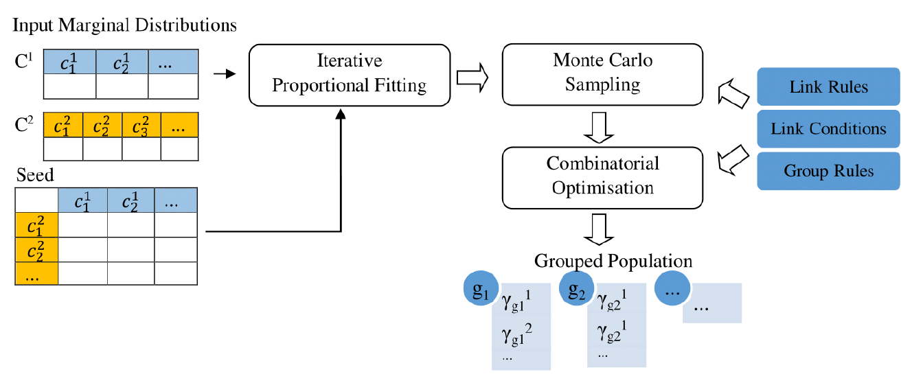
The proposed population construction framework consists of two phases. The first phase is merging distributions extracted from data sources using IPF, and the second is constructing groups based on the merged distribution. The Figure 1 provides an overview of the proposed methodology. The first part of the figure is the standard IPF distribution merging process. The IPF procedure takes two marginal distributions converted to the same aggregation level, annotated with \(C^1\) and \(C^2\), and a seed matrix as inputs and generates a joint distribution. If there are more than two distributions, though we have only shown two here, a multidimensional implementation of IPF can used[1]. The grouping process takes a joint distribution from IPF and a set of population heuristics via link rules, link conditions and group rules as inputs to produce group structures in the population. The following sections describe the steps for constructing the merged population.
Obtaining the marginal distributions
The first step is to identify the important population characteristics that need to be included in the merged population. For example, assume that three distributions of the number of persons by age, sex and relation- ship status from a data source on agent level population characteristics and a distribution of the number of persons by household size from a data source on household level characteristics are given. The objective is to construct a population by merging these distributions in a manner that preserves the structural properties of all the four input distributions. If multiple characteristics are chosen from the same data source it is recommended to query them as a joint distribution to minimise errors introduced during processing. If the distributions are frequencies of agents we convert them to probability distributions in preparation to run IPF on them. The reason for this is converting all the distributions to a common scale.
Definition 14. The probability distribution of agents in all categories of characteristic \(C^{i}\) is given by
| $$P(C^i): {\forall c^i \in C^i} \rightarrow \{x:x\in\mathbb{R}_{[0,1]}\}, \textrm{such that} \sum\limits_{\forall c^i \in C^i} P(C^i) = 1$$ |
Merging agent distributions
We employ IPF to obtain a joint probability distribution by merging the probability distributions derived from data sources. IPF relies on a disaggregated data sample of the target population, which is used as the seed (initial estimate of cell values). However, obtaining a disaggregated data sample on the population represented by marginal distributions is difficult due to data availability constraints. We propose circumventing this problem by indicating cells that can logically contain agents with 1s and cells that cannot contain agents with 0s. This is a deterministic assignment made based on domain knowledge. This abstract disaggregated data sample is represented by the seed matrix in the Figure 1. The data distributions are expected to be at the same aggregation level, though they may capture a hierarchy of concepts. For instance, when merging a person level distribution (e.g. age distribution) and a household level (e.g. household sized distribution), we expect the number of persons to be the counting unit of both populations. We denote the joint probability distribution constructed with IPF as I.
Given \(\Pi\) as the set of \(n\) probability distributions representing \(n\) characteristics obtained from data sources, the \(n\) dimensional joint probability distribution (\(I\)) is obtained by merging \(\Pi\) using IPF:
| $$I=\textrm{ipf}(\Pi,s)$$ | (1) |
The resulting joint probability distribution after running IPF is the representation of the merged population at the lowest aggregation level. We can get the merged agent population without group structures if we multiply the joint probability distribution (\(I\)) by the expected total number of agents and then instantiate the number of agents given in each cell with corresponding agent properties. If the population size is unknown, a suitable number has to be chosen based on domain knowledge. It has to be a reasonably large number to sufficiently capture important structural characteristics in the joint distribution. If the size of the target population is given as \(N\), the population distribution by the number of agents (\(S\)) is given as below.
| $$S = I \times N$$ | (2) |
Although the above process allows instantiating all the agents with the correct properties, it does not produce the group (social) structures in the population. For example, we can obtain all the agents in four member households using the above process, however, it will not give us information on the composition of household structures. So, there needs to be a mechanism to reconstruct group structures in the population.
Groups construction
The grouping process consists of two parts. The first part constructs an initial estimate of the group structures in the population using a process based on Monte Carlo Sampling as described in Algorithm 1. The second part is improving the solution with hill climbing optimisation. The approach proposed in this work is a heuristic algorithm that progresses using specified rules and observed distributions.
One of the inputs to the algorithm is the conditional probability distribution giving the probability of observing an agent of a certain agent type given its group type. Below is the function for obtaining conditional probability distribution from \(I\) probability distribution.
| $$P(A|G = g)= \begin{cases} \frac {I(A,G)} { \sum\limits_{a_{u} \in g} I(a_{u},g) }, & \text{if} \sum\limits_{a_{u} \in A} I(a_{u},g) > 0 \\ 0, & \text{otherwise} \end{cases}$$ | (3) |
| $$(a,g) = (c^1, ...,c^p,c^{p+1}, ..., c^{n}); c^1\in C^1, ..., c^n \in C^n$$ |
Here we first describe the Algorithm 1 at a high level before going into specific details. The algorithm iterates over all the group types constructing the expected number of groups under the selected group type in each iteration. A group is constructed in two phases. In the first phase, an agent is selected for the group and all its compulsory links are formed (lines 10-21) by adding suitable new agents to the group. For example, the marital relationship of a married person is a compulsory link. More specifically, compulsory links are given by the minimum number of a link type in an agent type’s link rules. If new agents were added to the group during the process their compulsory links are formed as well. This is continued until all compulsory links are formed for all of the agents in the group. After that we check the group type using function \(Q\) given in definition 12 (line 22). If the group has the expected group type it is added to the population, and we start forming a new group from the beginning. If not, the algorithm starts the second phase, where agents’ non-compulsory links are formed (lines 26-37). This phase iterates over the current agents in the group, in the order they appear, forming their non-compulsory links until the expected group type is achieved. We ensure that no link rule violations occur when adding new agents. Once the expected group type is achieved, the group is added to the population, if not it is discarded.
The inputs to the algorithm are Link Rules, Group Rules, the set of group types in the population, the conditional probability distribution (\(P(A|G = g)\)), the expected population distribution (\(S\)) and the maximum number of iterations allowed when forming groups (\(Itr_{max}\)). The output of the algorithm is the final population with group structures (\(\Gamma\)). Following functions and formalisms are used in the algorithm.
- \(|.|\) - size of any set or tuple
- \(type(a)\) - type of agent \(a\)
- \(min(l)\) - minimum required link instances for link type \(l\)
- \(max(l)\) - maximum allowed link instances for link type \(l\)
- \(R_L(r=type(a))\) - returns the link types and corresponding target agent types that agent \(a\) can form links with according to the link rules
- \(\gamma(\texttt{ref}=a,\texttt{link\_type}=l)\) - returns existing group members linked to agent \(a\) with a type \(l\) link in group \(\gamma\)
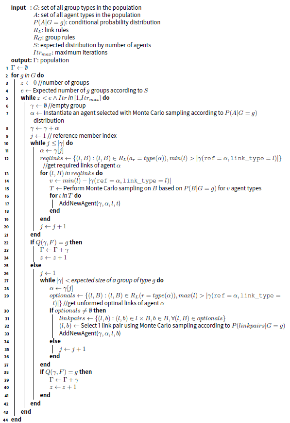
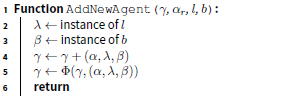
The algorithm starts by initialising the output population to an empty set. Then we select the first group type (\(g\)) from the set of all group types and start forming group instances (line 2). In line 4 we get the expected number of groups of the selected group type from \(S\). Initially the number of current groups (\(z\)) is set to 0. The algorithm keeps forming groups of current group type until the required number of groups are formed or it exceeds the maximum number of allowed iterations (line 5). The group being constructed is represented by \(\gamma\) and initially empty. The first agent of the group is selected using a Monte Carlo sampling technique based on the \((P(A|G = g)\) distribution of different agent types appearing in a group of the selected group type \(g\) (line 7). Here the \((P(A|G = g)\) distribution ensures that agent types not in the selected group type are not added to the group. Line 8 adds the new agent to the group and line 9 initialises index \(j\) to 1 to indicate the first member of the group. The next step is forming the minimum required links of the agents in the group. In line 11, we select the agent represented by \(j\)-th index in the group γ to form its required links. In the first iteration \(j\) refers to the new agent. The unformed required links of an agent can be found by taking the link types, in the agent’s link rules, that the minimum required number is larger than the agent’s existing links (line 12). Agents to form the missing links are selected using Monte Carlo sampling and added to the group (lines 13 - 19). Link conditions are applied whenever an agent is added to the group (Algorithm 2). This process is iterated for all the agents in the group until all the required links are formed.
If the group has fulfilled the requirements of the expected group type after forming all the required links it can be added to the population (line 22). Otherwise, the algorithm adds the missing number of agents by forming optional links of the existing agents until the group reaches the expected size. The expected size is assumed to be one of the group level characteristics (line 27). In line 29, we check whether the selected agent has formed the maximum allowed links from each link type it can form according to the link rules to identify optional links. Given that agents have formed all their required links during the first phase, any remaining link is considered an optional link. This computation is the same as finding the required links as described above except for \(max(l)\), which returns the maximum number of links allowed for link type \(l\). The output of the computation (\(optionals\)) is a set of ordered pairs representing a link type (\(l\)) and a set of target agent types (\(B\)) that \(a\) can form type \(l\) links. Though the same target agent type can be present in multiple pairs in the \(optionals\), they are considered different because the links they form are different. If the \(optionals\) set is not empty, we take all the different link type (\(l\)) and target agent type (\(b\)) pairs by taking the Cartesian product of each pair in the \(optionals\). The set of (\(l,b\)) pairs is represented by \(linkpairs\) (line 31). If the optional set is empty, we select the next agent in the group (line 35) and start forming its non-compulsory links. The link type and the target agent type is selected using Monte Carlo sampling according to the \(P(linkpairs|G=g)\) conditional probability distribution (line 32). The calculation given below shows how to obtain the conditional probability distribution of the \(linkpairs\) given \(g\) as the group type:
| $$P(linkpairs|G=g) = \begin{cases} \frac {P(A=b|G=g)} {\sum \limits_{\forall(l_u,b_{u}) \in linkpairs} P(A=b_{u}|G=g) }, & \sum \limits_{\forall(l_u,b_{u}) \in linkpairs} P(A=b_{u}|G=g) > 0\\ 0, & \text{otherwise}\end{cases}$$ | (4) |
| $$\forall(l,b)\in linkpairs$$ |
Once the required number of agents are added to the group, we check whether the group matches the expected group type using function \(Q\) and add it to the population if it is valid (lines 38 and 40). If the group does not match the expected group type it is discarded. This process is continued until all the groups are formed. At the end of this process, we have an initial estimate of the whole population.
The initial estimate of the population is improved using a standard hill climbing optimisation. The objective function used for hill climbing is based on the root mean squared error (RMSE). To calculate the error we define \(S_0\) as a function giving the total number of agents in the current reconstructed population, analogous to the function \(S\) given earlier, which represents the expected population. The RMSE calculation is given below. When proposing a change to the current estimate, we randomly select a group from the current population and construct a new group of the same type. The construction process for the new group has the same as logic explained from line 6 - 42 but instead of Monte Carlo sampling, here, we perform random sampling. In each case agent types are selected only when \(P(A|G=g) > 0\) and \(P(linkpairs|G=g) > 0\) to avoid adding agent types that do not appear under a group type. If swapping the new group with the old group improves RMSE we accept the change. This is continued until a RMSE = 0 achieved or the maximum number of iterations is exhausted.
| $$rmse(S_0) = \sqrt{ \frac{ \sum\limits_{a \in A} (S(a) - S_{0} (a))^2 }{ |A| } }$$ | (5) |
At the end of the process, we are given an agent population that is structurally similar to the input marginal distributions.
The population represents properties of person and household instances using the categories given in the input marginal distributions. In some situations, we have to assign persons and households specific values within a category. Age is such an example, as marginal distributions represent the population with age groups in most cases. We propose assigning an exact year to a person’s age using a suitable method considering relevant heuristics. For example, we may assign an age based on the number of persons by age (year) distribution of the population considering parent-child and marital partner age constraints.
Forming groups with subgroups
There are two ways to construct complex group structures that consist of multiple subgroups like multifamily households.
The first method is applying the proposed system iteratively on the population. Here, the process starts by constructing the subgroups of the lowest group aggregation level using the agent entities. After that subsequent iterations use the subgroups of the previous iteration as the agent entities to construct the groups of the next higher aggregation level. This approach requires specifying a new set of link rules, link conditions, group rules and marginal distributions representing agent and group entities for each iteration. In reference to a population of multifamily households, this method uses persons to form the families, in the first iteration, and the family instances to form the households, in the second iteration.
The second method is defining group rules at the highest group aggregation level while considering the composition of subgroups, so that the algorithm would form the complete groups in one iteration, while adhering to subgroup compositions. In this method, link rules and conditions are specified at the agent level and group rules are specified at the highest group aggregation level. For example, in a multifamily population link rules and link conditions specify relationships between persons and group rules specify household structures considering families in them. This method is more suited if data on subgroups are incomplete, for example, data on families in a household is incomplete or unavailable as this approach only requires marginal distributions at agent level (e.g. person level) and highest group aggregation level (e.g. household level). The second case study described below is an example of this approach.
Case Study 1: Merging Wedding Doughnut and Linked Lives Populations
Wedding Doughnut (WD) (Silverman et al. 2013) and Linked Lives (LL) (Noble et al. 2012) are two agent-based simulations modelling the UK population to evaluate social care needs. In this case study, we investigate constructing a common population by merging WD and LL populations. Similar work is also presented in (Wickramasinghe et al. 2017), however, they use a different algorithm and do not propose a framework for recording population heuristics. The purpose of this exercise is validating the proposed framework’s applicability in con- structing merged populations for integrated agent-based simulations.
The highlights of the WD model are its familial relationship representation and demographic processes. WD’s marital partnership formation model is based on social affinity of the agents. The spatial representation of the model is a toroidal space depicting agents’ social networks. The agents choose their partners based on their social affinity and partnership formations results in two agents moving to a location between their original locations. Its demographic process uses the Lee–Carter model and is guided by statistical data. The objective of LLis evaluating social care demand and supply amid changes in household structures. LLuses the Gompertz–Makeham mortality model and a flat reproductive probability for all 17 - 45 females. An abstract geographical representation of UK is used for the spatial representation. Agents can move from house to house within this space at different stages of life. Marital partnerships are formed between randomly selected persons.
A significant part of integrating ABMs is constructing an initial agent population consistent with all integrated models (Wickramasinghe et al. 2015). Here we apply the proposed methodology to construct a merged population for WD and LL. Based on the above analysis, we decided that the merged initial population should be consistent with the WD population’s age, gender and marital statuses distribution, and the LL population’s household sizes distribution. Table 1 gives the categories represented in the joint distribution extracted from WD.
The joint distribution of the person level (agent level) characteristics obtained from WD consists of 104 person types: 26 age categories with 4 year gaps \(\times\) two relationship status categories two categories \(\times\) based on gender. The categories under these characteristics are represented in Table 1. An example of a person type in the population is (Male, Married, 28-31), which is succinctly represented as (X1,M1,O8), using the category labels in Table 1. The only group level characteristic used in this population is the distribution of household sizes. Household types range from one member households (H1) to 12 member households (H12).
| Male (X1) | Female (X2) | ||||||||||
| Married (M1) | Single (M2) | Married (M1) | Single (M2) | ||||||||
| 0-3 (01) | ... | 100++ (026) | 0-3 (01) | ... | 100++ (026) | 0-3 (01) | ... | 100++(026) | 0-3 (01) | ... | 100++ (026) |
The first step of the population construction process is obtaining the conditional probability distribution of agent types in a given group type by merging the distributions obtained from the two models using IPF. To obtain the data distributions, we executed the WD and LL simulations independently and evolved them to the year 2011, so that the two populations conceptually represent the same UK population from a temporal point of view. At the year 2011, there were around 6900 persons in LL and 1000 in WD. The person level joint probability distribution was obtained from WD and the household level joint probability distribution from LL, by counting the number of persons that belong to different person and household types. The two distributions were then merged using IPF. The seed was constructed in the manner described in the Methodology section, where impossible cells were set to 0 and possible cells were set to 1. An example of an impossible cell is (Male, Single, 0-3) child living alone in a one person household. The IPF output is a matrix of proportions each cell representing the proportion of persons with a given combination of properties in the target population. This is the distribution presented by I in Equation 1 in the Methodology section. This distribution is converted to conditional probability distributions using Equation 3 taking household sizes as group types (g) and combinations of age, gender and marital status as agent types (a). To obtain the number of persons under each category the matrix is multiplied by the target population size, 4000 persons in this case (Equation 2).
Population heuristics
The population heuristics govern the relationships and household structures formed by the algorithm. Given the nature of WD and LL models, we assume that all the households are family households and that there are no unrelated individuals in them, except in one member households. Although the data extracted about households do not identify multifamily households, we have to allow them in the merged population to be able to create large households such as 12 person households. Following are the list of heuristics applicable to this case study, which are later represented as link rules and group rules.
- A person can have only one marital partnership.
- A person can have up to 8 children.
- A person can have only one father and one mother.
- A person over 16 years old can live alone.
- Only persons aged 16 years or more can form marital partnerships.
- A male can only have a marital partnership with a female from the same age category (group) or a category up to 15 years younger.
- A female can only have a marital partnership with a male from the same age category (group) or a category up to 15 years older.
- A child must be at least 15 years younger than the parent.
- Only persons aged 16 years or more can have children.
- All people in the household are related.
- The children of a person also considered children of the person’s partner.
- Household types are decided by households’ sizes.
Specifying link rules
The first step of defining link rules is identifying link types in the population. The link types in the population capture familial relationships among agents as heuristics 1 to 4 in the above list. These link types are sufficient in this case study because WD and LL only represent familial relationships. Table 2 gives all the link types used in the link rules. A None relationship is a representation of a non-existing relationship. This is used in the proposed population construction methodology for single persons living without any relatives in one member households.
| Link name | Minimum links | Maximum links | Description |
| MarriedTo | 1 | 1 | Marital relationship formed by a married person |
| MotherOf | 0 | 8 | maternal relationships a person forms with another person |
| FatherOf | 0 | 8 | paternal relationships a person forms with another person |
| ChildofFather | 0 | 1 | A person can have a father who is living in the same household |
| ChildofMother | 0 | 1 | A person can have a mother who is living in the same household |
| None | 0 | 0 | Indicates empty relationship - for single persons living alone |
Link rules for the population can be derived based on heuristics 5 to 10. For example, relationship types of (Male, Married, 28-31) person type are MarriedTo, FatherOf, ChildOfFather and ChildOfMother. When we consider marital relationships of the person type, marital partner needs to come from one of Female, Married, 16-19 to 28-31 person types. The FatherOfrelationships of the above person type can be formed with a person from any gender and marital status category, but in a younger age category with at least a 15 years gap. These and the remaining two link rules of (Male, Married, 28-31) person type are given in Table 3.
| Reference agent type | Link type | Target agent type |
| (X1,M1,O8) | MarriedTo | {(X2,M1,O5),(X2,M1,O6),(X2,M1,O7),(X2,M1,O8)} |
| (X1,M1,O8) | FatherOf | {(X1,M2,O1),(X1,M2,O2),(X1,M2,O3),(X1,M2,O4) (X2,M2,O1),(X2,M2,O2),(X2,M2,O3),(X2,M2,O4)} |
| (X1,M1,O8) | ChildOfFather | {(X1,M1,O13),(X1,M1,...),(X1,M1,O26), (X1,M2,O13),(X1,M2,...),(X1,M2,O26), |
| (X1,M1,O8) | ChildOfMother | {(X2,M1,O13),(X2,M1,...),(X2,M1,O26), (X2,M2,O13),(X2,M2,...),(X2,M2,O26)} |
| 1 | Link rules for males’ marital relationship \(\forall (X1,M1,O\omega)~\textrm{where}~\omega \in \{5, ..., 26\}\): \(((X1,M1,O\omega),\text{MarriedTo},\{(X2,M1,O\omega),(X2,M1,Ox), (X2,M1,O\epsilon)\}) , \epsilon = \begin{cases}\omega-3, & \text{if}\ \omega-3 \geq 5 \\5, & \text{otherwise}\end{cases}\) |
| 2 | Link rules for females’ marital relationship \(\forall (X2,M1,O\omega)~\textrm{where}~\omega \in \{5, ..., 26\}\): \(((X1,M1,O\omega),\text{MarriedTo},\{(X1,M1,O\omega),(X1,M1,Ox), (X\,M1,O\epsilon)\}) , \epsilon = \begin{cases}\omega+3, & \text{if}\ \omega+3 \geq 26 \\26, & \text{otherwise}\end{cases}\) |
| 3 | Link rules for paternal relationship of males \(\forall (X1,M\mu,O\omega)~\textrm{where}~\mu \in \{1,2\}\ \omega \in \{5, ..., 26\}\): \((X1,M\theta,O\omega),\text{FatherOf},{(X\nu,M\delta,O\omega -4),... (X\nu,M\delta,O1)}, \nu \in \{1,2\}, \delta \{1,2\}\) |
| 4 | Link rules for maternal relationship of females \(\forall (X2,M\mu,O\omega)~\textrm{where}~\mu \in \{1,2\}\ \omega \in \{5, ..., 26\}\): \((X2,M\mu,O\omega),\text{MotherOf},{(X\nu,M\delta,O\omega -4),... (X\nu,M\delta,O1)}, \nu \in \{1,2\}, \theta \{1,2\} \) |
| 5 | Link rules for persons’ relationship with the father \(\forall (X\theta,M\mu,O\omega)~\textrm{where}~\theta \in \{1,2\}\ \mu \in \{1, ..., 22\}\): \((X\theta,M\mu,O\omega),\text{ChildOfFather},{(X1, M\delta,O\omega +4),... (X1,M\delta,O26)}, \theta \in \{1,2\}\) |
| 6 | Link rules for persons’ relationship with the mother \(\forall (X\theta,M\mu,O\omega)~\textrm{where}~\theta \in \{1,2\}\ \omega \in \{1, ..., 22\}\): \((X\theta,M\mu,O\omega),\text{ChildOfMother},{(X2, M\delta,O\omega +4),... (X1,M\delta,O26)}, \theta \in \{1,2\}\) |
| 7 | Empty relationship of single persons living alone \(\forall (X\theta,M2,O\omega)~\textrm{where}~\theta \in \{1,2\}\ \omega \in \{5, ..., 26\}\): \(((X\theta,M2,O\omega),\text{NONE} ())\), |
As manually writing all the link rules is a cumbersome task, we automated the process using the statements shown in Table 4. The table gives all the link rules applicable to the WD and LL merging exercise. For instance, the statement in Row 1 gives the link rule for marital relationships of males. It first selects all the Male, Married and age 16 or over categories as the reference agent types. According to Table 1, age 16 or over categories are given by labels O5 to O26. X1 is the Male category and M1 is the Married category. The last line of the first row shows what agent types to be selected as potential target agent types relative to the reference agent type. Here the marital and gender categories of the target agent types are constant because partner must belong to Female (X2) and Married (M2) categories. However, the age categories that a partner can be selected change with reference agent type’s age because the heuristic specifies that the female partner of a male must be in the same or in a younger age category with no more than a 15 year gap. We represent this by taking married females from Oω to Os age categories, given male reference agent type’s age category is Oω (where s = ω 3). Additionally, we have also included a special condition to limit the youngest age category of a female partner to be 16-19 - O5 to avoid selecting person types younger than 15 years old for marital partnerships. The same approach was used to construct other link rule statements in Table 4.
Specifying group rules
The group types in the merged WD and LL population are the household types observed in the LL population distribution, which represents the number of persons in a household. Generating templates for all these household types is computationally expensive because person type combinations for a household grow exponentially with the household size. For example, there are 44 person types (44 combinations of person categories) that can form realistic one person households. More specifically, there are \(\binom{2}{1}\) ways to select one from two genders, \(\binom{1}{1}\) ways to select single persons (because married persons cannot live alone) and \(\binom{22}{1}\) ways to select one age category from 22 age categories that are over 15 years old. This amounts to \(\binom{2}{1} \times \binom{1}{1} \times \binom{22}{1} = 44\). When we consider two person households, there can be households of married couples or single parent households, which produce a total of 1094 household configurations. There are even more combinations for three member households. This computation is not feasible with resources available to most researchers. Our attempts to generate all the templates in this manner failed even with a system of 1TB RAM and 14 2.6GHz cores.
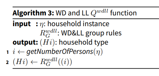
In this work, we avoid having to define a large number of household templates by taking the number of persons in the household as the unique feature that maps a given household to its type, as in definition 10. Here defining group rules is relatively simple because there is only one group level characteristic, household sizes distribution. Its categories are \(H1, H2,...,H12\). The corresponding features are the number of persons in a household, i.e. 1, 2, ..., 12. If \(i\) represents the household size, there is a heuristic function \(h\) to map household category to corresponding features.
| $$h:Hi \leftrightarrow \textrm{number of persons} $$ |
| $$R_G^{wdll}:\{(H1),(H2), ...,(H12)\} \leftrightarrow \{(1),(2), ..., (12)\}$$ |
| $$Q^{wdll}: (\eta,R_G^{wdll}) \rightarrow (Hi)$$ |
Specifying link conditions
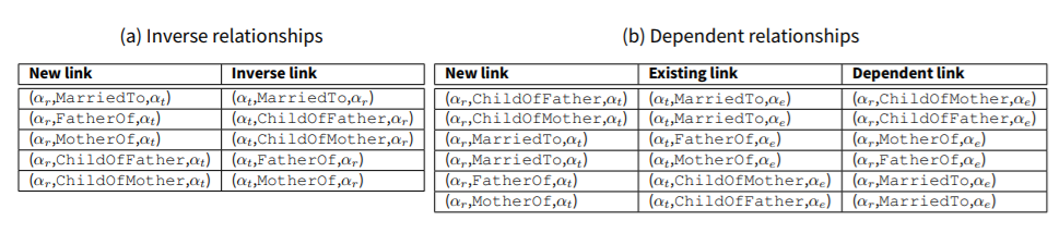
The heuristics captured in link conditions describe the new links that need to be formed as a result of forming another link. In relation to human relationships, we identify inverse relationships and dependent relationships as two types of link conditions. Inverse relationships capture the bidirectional nature of human relationships, for example, when a person of type (Female, Single, 32-35) is the MotherOf a (Male, Single, 4-7) person, the latter automatically becomes the child of the former, which is indicated as (Male, Single, 4-7) person is the ChildOf (Female, Single, 32-35) person.
The dependent relationships capture the situations where the formation of a relationship by person \(a_r\) with person \(a_t\) constitutes forming a new relationship between the person \(a_r\) and a person \(a_e\), because of an existing relationship between person \(a_t\) and \(a_e\). For example, given there exists a marital relationship between a (Male, Married, 32-35) person and a (Female, Married, 28-31) person, formation of a new ChildOfFather relationship by a (Female, Single, 0-3) person with a (Male, Married, 32-35) person requires forming a ChildOfMother relationship between the (Female, Single, 0-3) person and the (Female, Married, 28-31) person to maintain the consistency of relationships in the population. The relationships defined here are considered from the social/legal point of view and not from a biological point of view, so if two persons are married, children in their family form parental relationships with both of them.
Tables 5a and 5b give all the link conditions applicable to the merged WD and LL population. Here, \(a_r\) is the reference person who forms a new relationship, \(a_t\) is the target person with whom \(a_r\) forms the link and \(a_e\) is the person who has an existing relationship with \(a_t\). The inverse link and the dependent link represent the second link that needs to be formed as a condition of forming the new link.
 |
Results
We generated 100 pairs of WD and LL populations with different random seed values (for the random number generator) and used their marginal distributions to construct 100 merged population instances. The above specified link rules, link conditions, group rules and IPF seed matrix were used for merging all the population instances. Finally, for age, persons are assigned random years within their age category considering parent-child and marital partner age gap constraints.
To evaluate the results we compared each merged population’s joint distribution of the number of persons by gender, relationship status and age against the corresponding marginal distribution obtained from WD and the distribution of household sizes against the corresponding LLhousehold sizes distribution. When performing the tests we removed impossible person categories (e.g. male, married, age 0-3) from both the expected and observed distributions.
The goodness of fit of each constructed population was evaluated using the Freeman-Tukey goodness of fit test (Freeman & Tukey 1950). The test statistic is given by
| $$FT^{2}(O,E) = 4 \sum_{i}(\sqrt{O_{i}} - \sqrt{E_{i}})^{2}$$ |
Table 6 gives the results of the Freeman-Tukey goodness of fit test performed on marginal distributions of merged population instances against input WD and LL populations. Results show that none of the population instances were concluded inconsistent by rejecting the null hypothesis at 0.05 significance level. For person distributions all the instances had p-values over 0.95. However, this should not be interpreted as the synthesised population being a perfect match to the expected distribution, in fact still there are small errors between the synthesised and the expected distributions. At households level there was one borderline case with a p-value less than 0.1. However, 70 out of 100 had p-values over 0.85 with 59 of them being above 0.95. Table 6 also reports the mean and the standard deviation (SD) of the p-values. This shows that p-values are much larger than 0.05 significance level in most cases.
| Marginal | H0 rejected (p-value < 0.05) | Instances with p-value > 0.95 | Highest p-value | Lowest p-value | Mean | SD |
| WD | 0 | 100 | 1 | 1 | 1 | 0 |
| LL | 0 | 59 | 1 | 0.07117225 | 0.8734861 | 0.1848916 |
We further performed a power analysis on the test to explore the probability of detecting an effect in the reconstructed population when such an effect is actually present. For the test, we used 0.05 as the significance level, 4000 as sample size (the population size) and 0.1 effect size. The effect size was selected according to general guidelines provided by Cohen (1988) for social sciences where 0.1, 0.3 and 0.5 were proposed for small, medium and large effect sizes respectively. Table 7 gives the results of the power analysis. It shows that both tests will correctly reject the null hypothesis with a probability higher than the widely accepted 0.8 level when the probability of correctly rejecting the null hypothesis when it is false is set to 0.95. The probability of type II error in LL comparison test is only 0.0023 and in WD comparison test, the probability is 0.1951.
The population instance that resulted in the lowest p-value for the household level FT test is the 44th instance out of the 100. Plots in Figure 2 show the differences observed in this population instance. Figure 2a shows the differences in the number of households in the constructed population and the expected number of households as per input marginal distributions. The x-axis gives the household types, in this case, households of different sizes. The y-axis is the number of under/over represented households. However, the differences shown here are proportional values where integers are expected. The reason for this is round off errors introduced when multiplying the proportions in IPF result by the expected population size (Equation 2). The merged joint distribution (I) represents the population at lowest aggregation level, which in this case is persons. To get the number of households, we have to get the total persons under each household type and divide it by the expected number of persons in a household. This calculation sometimes results in a decimal number due to round off errors in previous steps. The errors we see in the plot are the proportional parts of these decimal numbers. The smaller sample sizes in households distribution also influence relatively low p-values.
| Marginal | Number of category combinations | Degrees of freedom | Power |
| WD | 96 | 95 | 0.8049 |
| LL | 12 | 11 | 0.9977 |
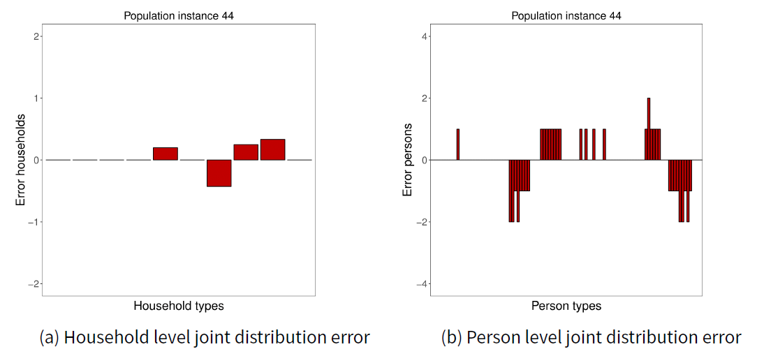
Figure 2b gives errors in the constructed population with respect to the expected person level joint marginal distribution of the 44th population instance. Y-axis gives the number of persons and x-axis gives the person types. The total absolute error in this constructed population instance with respect to person level distributions is 43 persons, which is about 0.01% out of all the persons. The errors are generally spread out among different person types with no particular person type having a significant enough error to reject the population as per FT test results.
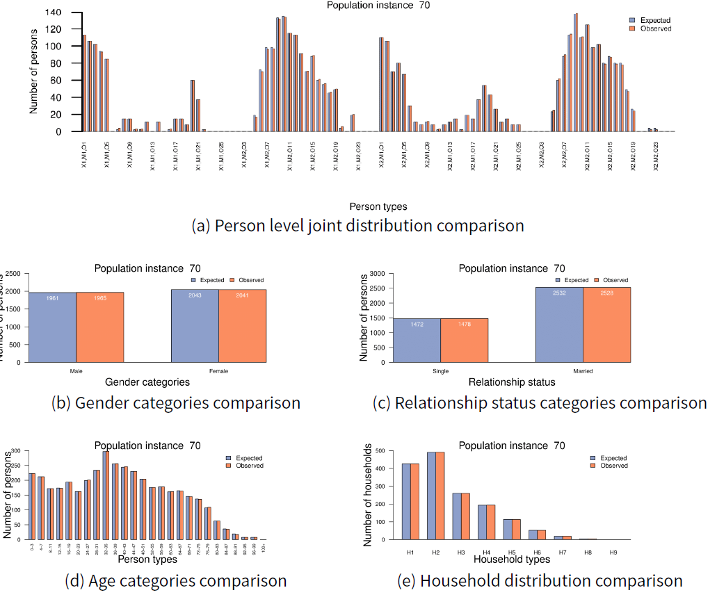
The graphs in Figure 3 show how structural characteristics of input distributions are preserved in 70th population instance, for which both LL and WD goodness of fit tests resulted in a p-value of 1. Figure 3a compares the expected and the observed joint distributions of all person level characteristics. The x-axis of the graph represents person types and the y-axis represents the number of persons. The x-axis labels refer to the categories given in Table 1. Here, we show only some of the labels due to space limitations. According to the graph, errors are relatively small in the reconstructed population and its structure is very similar to the input distribution, which supports the claim that populations synthesised using the algorithm are consistent with input distributions. Figures 3b, 3c and 3d show the structural consistency of person level characteristics individually. The characteristics used here are the distributions of the number of persons by gender, marital status, and age. Figure 3e compares the distribution of the number of households by sizes in the input and in the synthesised population. It is evident from the graphs that the populations constructed with the proposed methodology are structurally consistent with its input distributions.
In this case study, we demonstrated how the proposed framework can be used to construct an initial consistent agent population for integrated ABMs. While the algorithm produces promising results consistently, one of the reasons for observed mismatches is round off errors. Another factor is discrepancies in the two input distributions because they come from agent populations of different simulations, though we assume they conceptually represent the same population. Here we expect the algorithm to produce the best possible solution it can with the available data.
Case study 2: Population Construction Using Census Data
In this case study, we explore constructing a synthetic population by merging aggregated data from 2011 Australian census. Australian Statistical Geography Standard (ASGS) developed by Australian Bureau Statistics defines a hierarchical system that divides the country into smaller geographical areas[2]. Statistical Area 2 (SA2) is the third smallest area defined in the system and in most cases they correspond to officially gazetted state suburbs and localities. To construct the population we collected individual level and household level information of all SA2s that fall under the Greater Melbourne area in the state of Victoria. The proposed sample free technique is more desirable here, as any population generated with microdata samples would not be freely usable due to privacy restrictions.
Person level data
Individual level information collected under each SA2 includes joint distributions for the number of persons by age, gender and the person’s relationship in a household. There are 7 age categories, 6 relationship status categories and 2 gender categories. Table 8 gives the full list of categories under each characteristic. The labels prefixed with X,M and O are used in this document to refer to corresponding categories. The married category includes persons in a registered marriage or in a de facto partnership. Children category includes persons categorised as dependent students aged 15-24, dependent under 15 children and non-dependent children over 15 children. Relative is short for other related individuals, which encompasses individuals who live in the same household with a family but as not part of a family nucleus and persons related with relationships other than marital or parent/child relationships, for example, siblings. The relationship status of a person is decided in the prioritised order of marital, then parent/child, then relative relationships. Lone persons are the person living alone and group households are members of a households consisting only of non-related individuals like tenants. Additionally, though the Married category in census include persons in homosexual partnerships, for simplicity, we assume all married persons are in heterosexual partnerships. Also, parent/child relationships are treated from social/legal perspective rather than from the biological perspective. A complete description of the relationship types, family types and other special terms can be found in Australian Bureau of Statics website[3]. Here, a person type can be obtained by taking combinations of categories from each characteristic, for example (Male, Married, age 25-39) - (X1,M1,O3).
| Characteristic | Categories | ||||||
| Sex | Male (X1) | Female (X2) | |||||
| Relationship status | Married (M1) | Lone parent (M2) | Children (M3) | Group household (M4) | Lone person (M5) | Relative (M6) | |
| Age | 0-14 (O1) | 15-24 (O2) | 25-39 (O3) | 40-55 (O4) | 56-69 (O5) | 70-84 (O6) | 85+(O7) |
Household level data
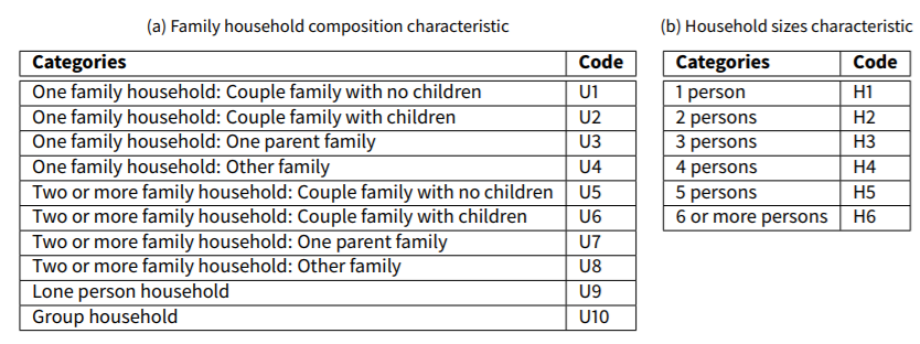
Household level information extracted for each SA2 includes the joint distribution of the number of persons by household size and family-household composition. Table 9 gives the categories under the two characteristics. Family household composition categories include the number of family units in the household and the type of the primary family unit. For example, Two or more family household: Couple family with no children refers to households with two or more family unit and the primary family is a couple family with no children unit. A household type in this case study is represented by a combination of house- hold size categories and family-household composition categories, for example, (4 person, One family household: One parent family) - (H4,U3).
A person belongs to only one family in the Australian census family categorisations and a household can have multiple families. A person’s family nucleus is determined in the prioritised order of the person’s marital relationship, parent/child relationships and other relationships. Any un-grouped children are added to the same family as their parents. In case of multi-generation parent/child relationships, ties are broken by prioritising the younger generation’s relationship, and the unmarried grandparent is categorised as a relative of the younger family. Same applies to older single parents of a married couple. The primary family of a multi-family household is selected in the prioritised order of couple family with children, one parent family and finally, couple family with no children and other family with equal priority.
Though the census identifies up to three family units in a household, the categories used here do not distinguish between households consisting of two and three families. They also do not distinguish among six to eight person households though the census does. The categories shown are selected to match the categories in disaggregated data samples available to us: in the interest of doing a more reasonable comparison with the sample data dependent IPU based population synthesiser proposed by Ye et al. (2009). It is noteworthy that the sample data can contain households of three families, and seven or eight persons though not categorised as such, this allows Ye et al. (2009)’s method to generate those households. These households are categorised under Two or more family households and six or more persons households accordingly. To generate a similar population with the proposed method, group rules are specified to categorise households with two and three family units as Two or more family households and households with six to eight persons as 6 or more persons households. If one needs fully descriptive family household composition categories there are no restrictions to specifying suitable group rules.
 |
We construct households in a single run by grouping persons directly considering both household and family compositions at once. Here, link rules specify persons’ relationships and group rules specify composite household and family structures. The alternative is constructing households in two iterations, one to form families using persons and the other to form households using families. This is not suitable here as marginal distributions only describe primary families, thus not enough information to construct all the families in the population in the first iteration. The approach used here also has the advantage of creating inter-family relationships of all the members in the household while assigning them to the correct family, whereas the other approach would create families as standalone units only with intra-family relationships of members, unless explicitly created as an ex post step.
Prior to constructing the population, the census data need to be cleaned to minimise the data inconsistencies. In Australian context, census data inconsistencies are caused either due to limitations in data collection process or deliberately introduced errors to protect privacy. Following is the list of heuristic adjustments made to the population to minimise the inconsistencies. It is important to note that data set is not descriptive enough to remove the inconsistencies completely. One such example is inability to know exact number of required married persons due to lack of information on secondary and tertiary family units in multifamily households.
- Set all unrealistic values to 0, e.g. (
Male, Married,age 0-15) and (3 person, Lone person household). - If the number of group household persons in person level data does not match with the number of persons expected according to household level data, update the person level group households distribution proportionally while preserving sex and age distribution.
- Proportionally update the number of lone persons in person level distribution to match persons required to form lone person households, if they are different.
- If the married number of males and females are different, proportionally increase the one with less per- sons to match the other.
- If there are not enough married males and females to form all primary family units that contain married couples, proportionally increase males and females in person level distribution.
- If number of lone parent persons is less than the number of lone parent family units in households, in- crease the lone parent persons proportionally to match the required number of persons.
- There must be enough children to form enough couple family with children and lone parent family units at least with one child in them. If not increase the number of children proportionally.
- If there are not enough relative persons to form all primary other-family units, increase the number of relative persons proportionally.
- If the total number of persons is less than the number of persons required by households, increase the persons proportionally. If there are more persons no changes are made due to the possibility of information loss.
Identifying population heuristics
The population construction starts by encoding the population heuristics using the constructs specified in the proposed framework. Following is the list of heuristics and assumptions describing important aspects of the population. They describe relationships between persons in the same household. The relationships across households are not represented in the available data, and we do not intend to represent them in the synthesised population. Here, an independent child is either a lone parent or a married person who is a child of another older lone parent or a married person. A dependent child is a person in the children category.
- A person can have a marital relationship with only one person.
- Only married or lone parent persons can have parental relationships.
- A lone parent must have at least one and a maximum of seven dependent children.
- A lone parent can have up to three independent children.
- A married person can have up to six dependent children.
- A married person can have up to three independent children.
- Married and lone parent persons can form none or up to three relationships with persons from “relative” category.
- A dependent child must have at least one parent in the same household.
- The only relationship that a group household person has with other members of the household is the relationship of living in the same household.
- Lone persons have no relationships.
- Persons in “relative” category cannot form any marital or parental relationships.
- Relatives can form one “relative of the family” relationship with a married or lone parent person.
- Relatives can form none or up to seven relationships with other “relative” type persons.
- By definition persons who fall under “children” category do not form marital partnerships or be a parent.
- Marital partnerships are assumed to be heterosexual relationships.
- A person must be over 15 years to form marital partnerships.
- A married male can have a marital relationship with a married female from the same age category or one below, and a married female can have marital relationship with a married male from the same age category or one above.
- A child is assumed to be 15 to 45 years younger than the parent.
- A group-household person can only be in a group household.
- The primary family is the family unit with most number of dependent children.
- Couple family with no children - must include two married persons. There can also be up to three relatives in the household. The three relatives have no relationship between them.
- Couple family with children - must include two married persons and at least one person from children category. The family can include up to three relatives who have no relationship between them.
- One parent family consists of a lone parent and at least one person from children category. The family can include up to three relatives who have no relationship between them.
- Only the primary family unit can have relatives.
- “Other-family” members consists of relative persons and the relationships between them cannot be categorised as either marital or parental.
- Lone person household consists of an adult person living alone.
- Group household only consists of persons from group-householder agent type.
- When a person forms a relationship with another person, the second person also forms a relationship with the first person. Both relationships are different point of views of the same conceptual relationship.
- The relationships in the population are not limited to biological ones and if a married person is also a parent of a child, the married person’s spouse is assumed as the other parent of the child.
- Every person in another-family is related to each other.
Specifying link types
When defining link types we consider the individual types that form the links and the types of households and families they form. Table 10 gives the link types identified in this exercise. The table gives the name of the relationships, a minimum and a maximum number of relationships that a person is allowed to form. In some cases, we have defined multiple different link types for the same conceptual relationship depending on the context. For example parent of relationship is divided into three link types considering parent agent’s type and child agent’s type because different heuristics apply in each case.
| Link name | Minimum | Maximum | Description |
| MarriedTo | 1 | 1 | Marital relationship formed by a married person |
| MarriedParentOfDependentChild | 0 | 6 | The relationship a married person can have with a dependent child. Dependent child is the category given by M3 in Table 8. Individual type married person may or may not have children. |
| LoneParentOfDependentChild | 1 | 7 | The relationship of a lone parent with their children. A lone parent must have at least one child. |
| ParentOfIndependentChild | 0 | 3 | The parental relationship between a parent and a person who is married or a lone par- ent. |
| DependentChildOf | 1 | 2 | The relationship that a dependent child forms with the parents. A dependent child must have a parent. |
| IndependentChildOf | 0 | 2 | The relationship that a married or a lone parent person forms with the parent. |
| GroupHouseholdOf | 1 | 7 | The relationship of persons living in a group household. The maximum group household size is 8. |
| FamilyRelative | 0 | 3 | The relationship formed by a Married or a Lone parent person with relatives who be- long to the same family unit. |
| FamilyRelativeInverse | 0 | 1 | The relationship formed by relative with a married or lone parent in the primary family. |
| RelativeOther | 0 | 7 | This is the relationship that persons in family type “other family” can have with each other. We allow “other family” family type to have up to 8 members. |
| None | 0 | 0 | Indicator for a null relationship. E.g. Lone person in a 1 member household |
Specifying link rules
Link rules determine the relationships that each person can form with other persons based on the person’s type. In the above heuristics list items from 1 to 19 describe the concerns that need to be encoded as link rules. Similar to the previous case study following is an example of a link rule that specifies a (Male, Relative, 85+) person type can have RelativeOther relationships with any Male (X1) or Female (X2) Relative (M6) person type from any age category (O1, ..., O7). We can specify similar link rules for all the agent types in the population.
| $$((X1,M6,O7), RelativeOther, \{(X1,M6,O1),(X1,M6,...), \\ (X1,M6,O7),(X2,M6,O1),(X2,M6,...),(X2,M6,O7)\})$$ |
The statements in Table 11 show how link rules can be generated for the first five link types given in Table 10. The link rules specified in the first row of Table 11 refer to marital partnerships that can be formed by male married persons of all ages. According to the heuristics, a person must be at least 15 years old to form marital partnerships. Because of that we only select married males in 2 (15-24) to 7 (85+) age categories. This is specified by the first statement in row 1. The second statement in the same row gives the link rules for male person types selected in line 1. The link rule specified that the females chosen for the marital partnership must be from the same age category or one category below. If the male’s age category is 15 - 24 (O2), then that person can only form a marital partnership with a female from the same age category, because persons of age 0 - 15 cannot form marital partnerships. The second row of the table gives link rules pertaining to marital partnerships of female persons. The other four rows show different link rules related to some parental relationships observed in the population. Similar logic can be specified for all the other link rules in the population. We can generate all the link rules easily by writing a simple script in this manner.
| 1 | Link rules for males' marital relationship \(\forall (X1,M1,O\omega)~\textrm{where}~\omega \in \{2, ..., 7\}:\) \(((X1,M1,O\omega),\texttt{MarriedTo},\{(X2,M1,O\omega),(X2,M1,Ox)\}) , x=\begin{cases}\omega-1, & \text{if}\ \omega \geq 3 \\2, \text{otherwise}\end{cases}\) |
| 2 | Link rules for females' marital relationship \(\forall (X2,M1,O\omega)~\textrm{where}~\omega \in \{2, ..., 7\}:\) \(((X2,M1,O\omega),\texttt{MarriedTo}, \{(X1,M1,O\omega),(X1,M1,...),(X1,M1,Ox)\}), x =\begin{cases}\omega+1, \text{if}\ \omega \leq 6 \\7, \text{otherwise}\end{cases}\) |
| 3 | Link rules for parental relationships of married persons' with dependent children
\(\forall (X\theta,M1,O\omega)~\text{where } \theta \in \{1,2\},\omega \in \{2, ..., 4\}:\) \(((X\theta,M1,O\omega),\texttt{MarriedParentOfDependentChild}, \{(X1,M3,O1),(X2,M3,O1)\})\) |
| 4 | Link rules for parental relationships of lone parents with dependent child
\(\forall (X\theta,M2,O\omega)~\text{where }\theta \in \{1,2\},\omega \in \{2, ..., 4\}:\) \(((X\theta,M2,O\omega),\texttt{LoneParentOfDependentChild}, \{(X1,M3,O1),(X2,M3,O1)\})\) |
| 5 | Link rules for parental relationships of married persons with Independent children
\(\forall (X1,M\mu,O\omega)~\text{where } \mu \in \{1,2\},\omega \in \{3, ..., 7\}:\) \(((X1,M\mu,O\omega),\texttt{ParentOfIndependentChild}, ((Xq,My,Ox), ..., (Xq,My,O\omega-1))), q\in\{1,2\}, y\in \{1,2\}, x = \begin{cases}% \omega-3, & \text{if}\ \omega \geq 6 |
| 6 | Link rules for parental relationships of lone parents with Independent children
\(\forall (X2,M\mu,O\omega)~\text{where } \mu \in \{1,2\},\omega \in \{3, ..., 7\}:\) |
| 7 | Link rules of dependent children with their parents
\(\forall (X\theta,M3,O1)~\text{where } \theta \in \{1,2\}:\) \(((X\theta,M3,O1),\texttt{DependentChildOf},\{(Xq,My,O2), ..., (Xq,My,O4)\}), q \in \{1,2\}, y\in\{1,2\}\) |
Specifying link conditions
The link condition types used here are similar to the ones used in the previous WD and LL case study because both are human populations. However, the actual link conditions are different because we use different link and person types in this population. The two types of link conditions are inverse links, capturing the bidirectional nature of human relationships, and dependent links, capturing dependencies on other existing relationships in a population. The items 28-30 in the above heuristics list relate to link conditions. Table 12 gives the two types of link conditions applicable to the census population. Here, \(a_r\), \(a_t\) and \(a_r\) indicate the agents that form the relationship. The first part shows the link conditions that need to apply because of the bidirectional nature of the human relationships. New link is the newly formed link and inverse link is the link formed because of the newlink. The second part of the table shows the relationships that need to be formed depending on the existing relationships of a participating agent. Existing link gives the already formed relationship and dependent link gives the relationship that needs to be formed when forming the new link.
| New link | Inverse link |
| \((a_r,\texttt{MarriedTo}, a_t)\) | \((a_t,\texttt{MarriedTo}, a_r\)) |
| \((a_r,\texttt{MarriedParentOfDependentChild}, a_t)\) | \((a_t,\texttt{DependentChild}, a_r\)) |
| \((a_r,\texttt{LoneParentOfDependentChild}, a_t)\) | \((a_t,\texttt{DependentChild}, a_r\)) |
| \((a_r,\texttt{ParentOfIndependentChild}, a_t)\) | \((a_t,\texttt{ParentOfIndependentChild}, a_r\)) |
| \((a_r,\texttt{DependentChild}, a_t)\) | If parent is married \(\rightarrow (a_t,\texttt{MarriedParentOfDependentChild}, a_r\)) If parent is a lone parent \(\rightarrow (a_t,\texttt{MarriedParentOfDependentChild}, a_r\)) |
| \((a_r,\texttt{GroupHouseholdOf}, a_t)\) | \((a_t,\texttt{GroupHouseholdOf}, a_r\)) |
| \((a_r,\texttt{FamilyRelative}, a_t)\) | \((a_t,\texttt{FamilyRelativeInverse}, a_r\)) |
| \((a_r,\texttt{FamilyRelativeInverse}, a_t)\) | \((a_t,\texttt{FamilyRelative}, a_r\)) |
| \((a_r,\texttt{RelativeOther}, a_t)\) | \((a_t,\texttt{RelativeOther}, a_r\)) |
| New link | Existing link | Dependent link |
| \((a_r,\texttt{MarriedTo}, a_t)\) | \((a_t,\texttt{MarriedParentOfDependendChild}, a_e\)) | \((a_r,\texttt{MarriedParentOfDependendChild}, a_e\)) |
| \((a_r,\texttt{MarriedTo}, a_t)\) | \((a_t,\texttt{ParentOfIndependendChild}, a_e\)) | \((a_r,\texttt{ParentOfIndependendChild}, a_e\)) |
| \((a_r,\texttt{MarriedParentOfDependentChild}, a_t)\) | \((a_t,\texttt{DependentChild}, a_e\)) | \((a_r,\texttt{ParentOfIndependendChild}, a_e\)) |
| \((a_r,\texttt{ParentOfIndependentChild}, a_t)\) | \((a_t,\texttt{IndependentChild}, a_e\)) | \((a_r,\texttt{MarriedTo}, a_e\)) |
| \((a_r,\texttt{DependendChildOf}, a_t)\) | \((a_t,\texttt{MarriedTo}, a_e\)) | \((a_r,\texttt{DependentChildOf}, a_e\)) |
| \((a_r,\texttt{IndependendChildOf}, a_t)\) | \((a_t,\texttt{MarriedTo}, a_e\)) | \((a_r,\texttt{IndependentChildOf}, a_e\)) |
| \((a_r,\texttt{GroupHouseholdOf}, a_t)\) | \((a_t,\texttt{GroupHouseholdOf}, a_e\)) | \((a_r,\texttt{GroupHouseholdOf}, a_e\)) |
| \((a_r,\texttt{RelativeOther}, a_t)\) | \((a_t,\texttt{RelativeOther}, a_e\)) | \((a_r,\texttt{RelativeOther}, a_e\)) |
Specifying group rules
Group rules determine the type of a given household. In this exercise, the features used to determine household type are the household size and the household composition. The latter feature considers the number of family units, the primary family’s type and whether the households members are related individuals. The family units in the population are: couple family with children, couple family without children, lone parent family, and other family. Group households and lone persons are non-family units observed in households. Heuristics on household composition are given in lines 20-27 in the above heuristics list.
Group rules function (\(R_G^{census}\)), formulated as per definition 11, determines household type considering the two group level characteristics in the data: household size and family household composition (number of family units and primary family unit type). Given \(Hi\) represents a household size category, heuristic function for mapping features with household sizes is same as the previous case study (\(i \in \mathbb{Z}^+{[1,8]}\)).
| $$H^{i}:Hi \leftrightarrow \textrm{number of persons}$$ |
group household person type the household is considered a group household and all the members are considered to be part of one family unit. For lone person households the person alone is considered a lone person family. Apart from above, following agent compositions are considered basic family units: married couple, a lone parent with a child and two relatives with relative other relationships. The number of family units can be identified by counting these agent compositions. The family type of the first person added to the household is considered the primary family type. If the first person’s family nucleus consists of a married couple that has at least one child, the family type is couple with children family, if there are no children then it is a couple only family . If there is a lone parent in the family nucleus it is considered a Lone parent family. If there are relatives with relative other relationships then the family type is other family. Below two heuristic functions are formulated according to definition 10. Here U1 refer to One family household: Couple family with no children category and U10 refer to Group household category.
| $$H^{9}:U1\leftrightarrow \textrm{1 family unit, primary family has two}\, \texttt{married}\, \textrm{persons but no}\, \texttt{children}$$ |
| $$H^{22}:U10 \leftrightarrow \textrm{Household members belong to}\, \texttt{group household}\, \textrm{person type}$$ |
The group rules set for census population can be represented in following manner:
| $$R_G^{census}: H \times U \leftrightarrow \{\textrm{set of different number of persons}\}\times \{\textrm{agent compositions}\}$$ |
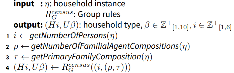
The population of an SA2 is constructed by running the program with the above specified link rules, group rules, link conditions, marginal distributions from census data and the seed. To perform the IPF step, which requires both distributions to be at the same aggregation level, we obtained the number of persons in a household type by multiplying the household distribution by the household size. The seed here is a two dimensional matrix corresponding to two joint distributions used for the population. The cell values are deterministically assigned 1s and 0s indicating possible and impossible cells as described previously. The only input that needs to be changed for different SA2s is the set of marginal distributions from census data. Link rules, link conditions, group rules and the seed do not change as they are based on common population heuristics.
To assign a year to a person’s age property, we selected a year within the person’s age category according to the number of persons by age (year) distribution of each SA2. Age assignment further considered relevant population heuristics related to person’s age.
Results
As the method is guaranteed to only generate legal household configurations according to the specified rules, main focus of this section is the structural aspects of the synthesised population. First, we illustrate that the synthesised populations are similar to the input distributions and then, we show that, our method generates statistically superior populations than the IPU based method described by Ye et al. (2009).
We selected 16 SA2s from Darebin and Banyule local government areas and for each person and household distribution pair constructed 20 different synthetic populations with varying random seed values. The distribution of persons of a constructed population was obtained by counting the number of persons that fall under each person type and household distribution counting the number of households under each household category. The goodness of fit of each synthesised population was evaluated using FT test. Categories that represent impossible person types (e.g. (Male, Married, age 0-15)) and household types (e.g. 1 person, 2 families: couple family with children ) are not included in the tests. So the number of person categories used for the tests reduced from 84 to 76 and household type categories from 60 to 36.
Table 13 presents the FT test outcome with the H0 rejected of population instances out of 20, the highest observed p-value, the lowest observed p-value, the mean over the 20 p-values and the standard deviation (SD) for each SA2. The degrees of freedom for the person level FT tests is 75 and for the household level is 35. In the table none of the population instances were deemed inconsistent, in fact, the p-values of all the population instances shown in the table are over 0.95, which is very promising. Very small standard deviations indicate that the algorithm’s results are consistent and multiple runs are not required to obtain the best result in most cases. Below, we further compare synthesised population to the census distributions using q-q plots.
| SA2 | Person level | Household level | ||||||||
| H0 rejected (p-value < 0.05) | Maximum p-value | Minimum p-value | Mean | SD | H0 rejected (p-value < 0.05) | Maximum p-value | Minimum p-value | Mean | SD | |
| Alphington - Fairfield | 0 | 1 | 1 | 1 | 0 | 0 | 1 | 1 | 1 | 0 |
| Bundoora - East | 0 | 1 | 1 | 1 | 0 | 0 | 1 | 1 | 1 | 0 |
| Greensborough | 0 | 0.9999 | 0.9979 | 0.9997 | 0.0006 | 0 | 1 | 1 | 1 | 0 |
| Heidelberg - Rosanna | 0 | 1 | 0.9999 | 0.9999 | 6.23×10⁻¹⁴ | 0 | 1 | 1 | 1 | 0 |
| Heidelberg West | 0 | 1 | 1 | 1 | 0 | 0 | 1 | 1 | 1 | 0 |
| Ivanhoe | 0 | 1 | 1 | 1 | 0 | 0 | 1 | 1 | 1 | 0 |
| Ivanhoe East - Eaglemont | 0 | 1 | 0.9999 | 0.9999 | 3.15×10⁻⁷ | 0 | 1 | 1 | 1 | 0 |
| Kingsbury | 0 | 1 | 1 | 1 | 0 | 0 | 1 | 1 | 1 | 0 |
| Montmorency - Briar Hill | 0 | 0.9999 | 0.9999 | 0.9999 | 4.17×10⁻⁶ | 0 | 1 | 1 | 1 | 0 |
| Northcote | 0 | 1 | 0.9999 | 0.9999 | 2.34×10⁻⁹ | 0 | 1 | 1 | 1 | 0 |
| Preston | 0 | 0.9999 | 0.9999 | 0.9999 | 2.6 ×10⁻⁹ | 0 | 1 | 1 | 1 | 0 |
| Reservoir - East | 0 | 1 | 1 | 1 | 0 | 0 | 1 | 1 | 1 | 0 |
| Reservoir - West | 0 | 1 | 1 | 1 | 0 | 0 | 0.9998 | 0.9998 | 0.9998 | 0 |
| Thornbury | 0 | 1 | 0.9999 | 0.9999 | 2.18×10⁻¹⁵ | 0 | 1 | 1 | 1 | 0 |
| Viewbank - Yallambie | 0 | 1 | 0.9999 | 0.9999 | 5.19 ×10⁻¹⁰ | 0 | 1 | 1 | 1 | 0 |
| Watsonia | 0 | 1 | 0.9999 | 0.9999 | 4.93×10⁻¹⁵ | 0 | 1 | 1 | 1 | 0 |
The post hoc power analysis showed high power in all the cases of individual level FT tests. We used 0.05 significant level, 83 degrees of freedom (because there are 84 agent types) and a small effect size of 0.12 according to guidelines proposed by Cohen (1988). All the tests have very high power in this exercise because of large population sizes (sample size). The lowest power was observed in the tests conducted on Ivanhoe East - Eaglemont SA2, which is 0.99996 (population size = 7207). This indicates 0.00004 probability of type II error. Additionally, 7 SA2s resulted in a power of 1 because of their relatively large population size. For power analysis of tests on household level distributions, we used the same significant level and effect size, but for 59 degrees of freedom because corresponding to 60 household types. The lowest power was again observed in tests conducted on Ivanhoe East - Eaglemont SA2, which is 0.8866, a probability of 0.1134 type II error, again attributed to the relatively small population. The highest power of 0.9999 was observed for Preston.
Figure 4 shows the quantile-quantile plot for one of the population instances constructed for arbitrarily selected Thornbury SA2. A point in the Figure 4a represents a person type in the population and the \(y = x\) trend line is represented in red. A point’s \(x\) projection is the number of persons in pre-processed census input and y projection is the number of persons in the synthesised. If the number of persons in a person type is equal in both census and synthesised, the corresponding point falls right on the \(y = x\) trend line. The Figure 4b compares household distributions of the same population. The figure shows that in both cases person type and household type points fall very close to the \(y = x\) trend line.
The proposed algorithm produced satisfactory results in most of the experiments. However, there are cases where complex family structures are not constructed, for instance, three Five persons, Two or more family household: Other family instances were not formed in Reservoir - West, hence the relatively low p-value. Another possible reason for this is the low probability of selecting a Relative when forming families due to having very few in the census distribution.
Comparison to IPU based population synthesis
In this section we compare the proposed approach to the Iterative Proportional Updating (IPU) based method discussed in Ye et al. (2009). The IPU based method generates synthetic populations that match person and household level marginal distributions similar to the proposed approach, but using a disaggregated sample. The IPU implementation used here is available in Urban Data Science Toolkit [4].
For the evaluation, we obtained 1% microdata samples of the 9 SA4 areas covering Greater Melbourne, which fully encompass the 278 SA2 areas, under strict obligations not to share any disaggregated data. An SA4 consists of multiple non-overlapping SA2s. The person and household marginal distributions were same as before. To generate SA2 populations with IPU based method we used the whole microdata sample of the corresponding SA4 area and selected the best out of 20 runs as proposed by Ye et al. (2009). The number of IPU iterations were also increased to 20,000 to allow the algorithm to achieve the 0.0001 goodness of fit level. For our algorithm generating one population instance per SA2 was deemed sufficient as there are minimal variations across different runs according to the Table 13.
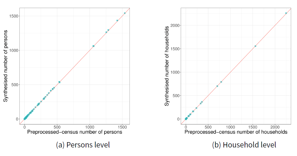
| Marginal distributions | Our | IPU | ||
| p-value < 0.05 | p-value > 0.95 | p-value < 0.05 | p-value > 0.95 | |
| Household level | 0 | 271 | 156 | 52 |
| Person level | 2 | 273 | 14 | 202 |
| Independent characteristic | Our | IPU | ||
| p-value < 0.05 | p-value > 0.95 | p-value < 0.05 | p-value > 0.95 | |
| Household size | 0 | 278 | 4 | 233 |
| Family composition | 0 | 278 | 12 | 81 |
| Relationship status | 21 | 128 | 61 | 43 |
| Sex | 0 | 84 | 40 | 0 |
| Age | 1 | 273 | 36 | 14 |
The Table 14a shows that 97.5% (271 out of 278) of the population instances generated with our algorithm had p- values over 0.95 at household level and 98% (273) at person level, but with IPU based method only 52 (19%) SA2s produced p-values above 0.95 at household level and 202 (72.5%) at person level. It is also important to note that more than half (156) of the IPU generated populations are inconsistent at household level, while none with our algorithm. At person level only 2 (0.08%) SA2s produced different population with our algorithm, but IPU based method produced 14 (5%).
Brighton (Vic.) and Eltham are the two SA2s that have significantly different synthesised populations of our algorithm at person level. Their p-values are 0.029 and 0.002. The census distributions of all SA2s have discrepancies between the number of persons required to form the households and the number in the persons distribution, that in this two SA2s are, respectively, 436 and 557 persons, comparatively large numbers but only about a 0.02% error considering each SA2’s population size. However, the algorithm has successfully handled much larger errors in other SA2s. Another common observation is that Married and Children categories
are the highest contributors to errors in the synthesised populations. Further investigations are required to understand the exact reasons why these two SA2s fail to produce satisfactory results.
In the Table 14b we further analyse how well the two algorithms have preserved individual characteristics of each joint marginal distribution obtained from census data. Results show that our method preserves the distributions of individual characteristics comparatively better than the IPU based method. Sex characteristic shows weaker results in both methods, as a result of having only two categories under it causing errors to be prominent when tested.
In general IPU based method’s results reported here is weaker than reported by Ye et al. (2009). Apart from the obvious difference of the two populations, our experiments are different to them because: a) zero household and person categories are not removed when synthesising the populations, b) a different statistical test is used and c) only impossible categories are removed from the statistical evaluation. It is also noteworthy that they have reported detailed results of only two blockgroup areas though the population was constructed for a much larger area.
Current prototype implementation of the algorithm on average takes about five minutes for an SA2 on a computer with a Core i5 - 2.40 GHz processor and 4GB RAM. This is slower than the 2 minutes that IPU based method takes for the whole population. While there is room to improve the efficiency, the current implementation is still usable given the high accuracy rate and the synthetic population has to be generated only once for any simulation. The source code is available on Github[5].
Discussion
The paper proposed an application independent heuristic methodology for reconstructing agent populations with social structures without depending on disaggregated data samples. The methodology consists of a generic framework for specifying application heuristics and an algorithm that uses the framework constructs to synthesise the population. The main constructs specified in the framework are link rules, group rules and link conditions. The group construction process takes binned data distributions from different sources and produces the population by forming group structures according to the heuristics specified through the three framework constructs. The main steps of the process are merging the data distributions with IPF using an abstract seed, constructing an initial estimate of the group structures in the population based on Monte Carlo sampling according to input distributions, and improving the initial estimate using a combinatorial optimisation technique. Currently, the approach requires converting both distributions to the same aggregation level due its dependency on IPF. Heuristics specification framework, however, does not have be in the same aggregation level.
We demonstrated the versatility of the proposed approach by applying it to two case studies. The first one caters the interests in building integrated agent-based models (Singh & Padgham 2014; Wickramasinghe et al. 2015), by merging two populations from different ABMs to obtain a consistent merged population. The second case study constructs a synthetic population using Australian census data. These show that the proposed method can be used in different applications simply by changing heuristics via the framework without developing a completely new program. Freeman Tukey’s goodness of fit test results indicate highly consistent results out performing state-of-the-art IPU (Ye et al. 2009) based approach.
The main contribution of this work is the generic heuristics specification framework. It allows generating different populations by changing the population heuristics without changing the underlying population construction algorithm, where as, existing sample-free heuristic population synthesis algorithms would require re-writing population synthesis logic completely. Though a similar work is also discussed in (Wickramasinghe et al. 2017), it does not elaborate the generic heuristic framework and the algorithm is different to we have presented here.
Using IPF to merge data distributions is a common approach in synthetic population construction. However, in this work, we approximate the seed to a matrix of 1s and 0s indicating possible and impossible cells. Lovelace et al. (2015) experimentally show that initial weights in the matrix have no significant influence on the final IPF outcome after 10 iterations. While it can be argued that the difference between the abstract seed we use and the correct hypothetical seed is rather extreme than the seed errors introduced in Lovelace et. al’s experiments, our results suggest that the proposed abstract seed is still viable, especially given that there is no suitable disaggregated data sample.
Future work will primarily explore on removing the constraint of having all the marginal distributions in the same aggregation level by coupling the heuristic framework with a multilevel method like IPU and Hierarchical IPF, or using the marginal distributions without merging them with a IPF like technique, similar to the probabilistic selection method of Gargiulo et al. (2010). Additionally, we will also explore iteratively applying the algorithm to construct populations of multiple hierarchies and complex group structures. Another avenue would be developing a domain specific language for specifying link rules, group rules and link conditions.
Notes
- https://cran.r-project.org/web/packages/mipfp/.
- www.abs.gov.au/ausstats/abs@.nsf/Lookup/2901.0Chapter23102011.
- www.abs.gov.au/ausstats/abs@.nsf/Previousproducts/2901.0Main%20Features702011.
- https://github.com/UDST/synthpop.
- https://github.com/denizens/freesyn.
References
BALLAS, D., Clarke, G. P. & Turton, I. (2003). 'A spatial microsimulation model for social policy evaluation.' In B. Boots, A. Okabe & R. Thomas (Eds.), Modelling Geographical SystemsBerlin/Heidelberg: Springer, pp. 143–168. [doi:10.1007/978-94-017-2296-4_8]
BARTHELEMY, J. & Toint, P. L. (2013). Synthetic Population Generation Without a Sample. Transportation Science, 47(2), 266–279.
BECKMAN, R. J., Baggerly, K. a. & McKay, M. D. (1996). Creating synthetic baseline populations. Transportation Research Part A: Policy and Practice, 30(6), 415–429 [doi:10.1016/0965-8564(96)00004-3]
COHEN, J. (1988). Statistical Power Analysis for the Behavioral Sciences. Journal of the American Statistical Association, 84(408), 1096
DAHMANN, J., Fujimoto, R. & Weatherly, R. (1998). The DoD High Level Architecture: an update. In 1998 Winter Simulation Conference. Proceedings (Cat. No.98CH36274), vol. 1, (pp. 797–804). IEEE. [doi:10.1109/WSC.1998.745066]
DEMING, W. E. & Stephan, F. F. (1940). On a Least Squares Adjustment of a Sampled Frequency Table When the Expected Marginal Totals are Known. The Annals of Mathematical Statistics, 11(4), 427–444.
ETTEMA, D. (2011). A multi-agent model of urban processes: Modelling relocation processes and price setting in housing markets. Computers, Environment and Urban Systems, 35(1), 1–11. [doi:10.1016/j.compenvurbsys.2010.06.005]
FAROOQ, B., Bierlaire, M., Hurtubia, R. & Flötteröd, G. (2013). Simulation based population synthesis. Transportation Research Part B: Methodological, 58, 243–263.
FREEMAN, M. F. & Tukey, J. W. (1950). Transformations Related to the Angular and the Square Root. The Annals of Mathematical Statistics, 21(4), 607–611. [doi:10.1214/aoms/1177729756]
GARGIULO, F., Ternes, S., Huet, S. & Deuuant, G. (2010). An iterative approach for generating statistically realistic populations of households. PLoS ONE, 5(1): e8828.
HUYNH, N., Barthelemy, J. & Perez, P. (2016). A Heuristic Combinatorial Optimisation Approach to Synthesising a Population for Agent-based Modelling Purposes. Journal of Artificial Societies and Social Simulation, 19(4), 11: https://www.jasss.org/19/4/11.html. [doi:10.18564/jasss.3198]
KIRILL, M. & Axhausen, K. W. (2011). Hierarchical IPF: Generating a synthetic population for Switzerland. 51st Congress of the European Regional Science Association, January. European Regional Science Association (ERSA).
LOVELACE, R., Ballas, D., Birkin, M. & van Leeuwen, E. (2015). Evaluating the performance of Iterative Proportional Fitting for spatial microsimulation: new tests for an established technique. Journal of Artificial Societies and Social Simulation, 18(2), 21: https://www.jasss.org/18/2/21.html. [doi:10.18564/jasss.2768]
NAMAZI-RAD, M. R., Mokhtarian, P. & Perez, P. (2014). Generating a dynamic synthetic population - Using an age- structured two-sex model for household dynamics. PLoS ONE, 9(4): e94761.
NOBLE, J., Silverman, E., Bijak, J., Rossiter, S., Evandrou, M., Bullock, S., Vlachantoni, A. & Falkingham, J. (2012). Linked lives: The utility of an agent-based approach to modeling partnership and household formation in the context of social care. In 2012 Winter Simulation Conference (WSC), 2011, (pp. 1–12). IEEE [doi:10.1109/WSC.2012.6465264]
RANEY, B. & Nagel, K. (2006). 'An improved framework for large-scale multi-agent simulations of travel behaviour.' In Rietveld, P. Jourquin, B. & Westin, K. (Eds.), Towards Better Performing European Transportation Systems. London: Routledge, pp. 305–347.
SCHELLING, T. C. (1971). Dynamic models of segregation. The Journal of Mathematical Sociology, 1(2), 143–186. [doi:10.1080/0022250X.1971.9989794]
SILVERMAN, E., Bijak, J., Hilton, J., Cao, V. D. & Noble, J. (2013). When demography met social simulation: A tale of two modelling approaches. Journal of Artificial Societies and Social Simulation, 16(4), 9: https://www.jasss.org/16/4/9.html. [doi:10.18564/jasss.2327]
SINGH, D. & Padgham, L. (2014). OpenSim: framework for integrating agent-based models and simulation components. In Proceedings of the European Conference on Artificial Intelligence (ECAI), (pp. 837–842). Prague, Czech Republic.
SMITH, A. P., Lovelace, R. & Birkin, M. (2017). Population synthesis with quasirandom integer sampling. Journal of Artificial Societies and Social Simulation, 20(4), 14: https://www.jasss.org/20/4/14.html.
TANTON, R., Vidyattama, Y., Nepal, B. & McNamara, J. (2011). Small area estimation using a reweighting algorithm. Journal of the Royal Statistical Society. Series A (Statistics in Society), 174(4), 931–951. [doi:10.1111/j.1467-985X.2011.00690.x]
VOAS, D. & Williamson, P. (2001). Evaluating goodness-of-fit measures for synthetic microdata. Geographical and Environmental Modelling, 5(2), 177–200.
WICKRAMASINGHE, B. N., Singh, D. & Padgham, L. (2015). Synchronising Agent Populations when Combining Agent-Based Simulations. In Spring Simulation Multiconference. Alexandria, USA.
WICKRAMASINGHE, B. N., Singh, D. & Padgham, L. (2017). Heuristic Data Merging for Constructing Initial Agent Populations. In J. A. R.-A. Gita Sukthankar (Ed.), AAMAS 2017 Workshops Visionary Papers. Sao Paulo: Springer International Publishing.
WILLIAMSON, P., Birkin, M. & Rees, P. H. (1998). The estimation of population microdata by using data from small area statistics and samples of anonymised records. Environment and Planning A, 30(5), 785–816. [doi:10.1068/a300785]
YE, P., Hu, X., Yuan, Y. & Wang, F.-Y. (2017). Population Synthesis Based on Joint Distribution Inference Without Disaggregate Samples. Journal of Artificial Societies and Social Simulation, 20(4), 16: https://www.jasss.org/20/4/16.html, [doi:10.18564/jasss.3533]
YE, X., Konduri, K., Pendyala, R. & Sana, B. (2009). A methodology to match distributions of both household and person attributes in the generation of synthetic populations. 88th Annual Meeting of the Transportation Research Board, 9600(206).