
Introduction
Sustainable consumption is a matter of great and current interest. It includes a series of behaviour and actions aimed at achieving greater environmental compatibility of the consumer goods-life cycle. Sustainable food consumption has various objectives, including reducing consumption of non-renewable resources and preserving them over time, producing less pollution, generating less waste, shortening the product distribution chain and educating people on good consumer practices (Goryńska-Goldmann et al. 2016; Annunziata and Scarpato 2014). For the consumer, all this entails a rethinking of consumption practices: i.e., increasing the share of fresh and seasonal products, looking for local products rather than exotic ones, increasing nutrition and gastronomic skills, changing established dietary schemes, and in general, having greater environmental awareness of buying choices (Verain et al. 2015; Annunziata and Scarpato 2014; Brunori and Lari 2012).
To achieve these objectives, food retail shops can focus on food diversification and specialization (in relation to the more standardized supply of supermarkets) and on the supply of local and fresh products. These food retail shops are generally small and are not a quantitative alternative to the consolidated forms of distribution represented by supermarkets. However, they do generally represent a stimulus to innovation in the food supply chain and also for supermarkets that can emulate this type of supply (Mikkola 2015). Yet the small size of these shops is a great problem for their survival, as shown by the general and established tendency toward the closure of small businesses due to ruthless competition from supermarkets (Borraz et al. 2014).
Aim of the Study
What dynamics could the opening of a small food shop trigger in the local competitive environment? What are the implications for the grocery sector? In trying to answer these questions, this study has attempted to provide a forecasting simulation method, to understand how a small shop can survive in the retail food market competition in a local context. The method consists of an agent-based model (ABM) for the dynamic representation of the competitive and social environment in that local context, reproducing the current state of the consumer food market. Events can be entered into this state, such as opening new stores and launching promotional campaigns, providing us with the opportunity to see how the situation is changed by these events.
The model is based on the relationship between consumer and store (business to consumer exchanges) and does not deal with individual food items, but rather with all products that make up consumer food expenditure, which can be defined as the “food basket”. The agents of the model belong to two categories: consumers and retailers. The implementation of the model pursues specific goals that can be summarized as follows:
- reproduce the consumer’s decision-making process, based on a plurality of attributes that interact to define consumer behaviour;
- implement a process of diffusion of innovations in the market, through the exchange of opinions inside the consumer network, allowing a simulation of the real dynamics of the process and changes induced by them;
- understand the relationships and dynamics on a geographical basis, according to the location of various agents.
Alongside these specific goals, the model also has some more general objectives, which are to
- use a methodology of recent and promising development, (ABMs), in the specific context of studying the food supply chain, particularly as a means to understand the complex interactions that exist within this sector, in order to grasp the dynamics of the market and check their effects;
- identify the types of data needed to construct the model and to direct market research and data collection necessary to design action in the food market similar to the one under study;
- provide support for solutions to the known problems of excessive fragmentation of the chain, especially in regards to the distribution phase.
The Case Study
As a case study, the model simulates the opening of a farmers’ market (FM) in a hypothetical urban area that reflects the population density of a medium-sized town in central Italy. The FM can be an interesting case study as it fits the competitive landscape without a pre-established scheme, so its opening could alter competitors’ previously made break-even analyses. The FM is a significant example of a retail shop following the scope of sustainable consumption. Furthermore, the typical Italian FM can be considered a small shop, due to its low revenue level (Filippini and Zucconi 2009).
By putting the producer and consumer into direct communication with each other, FMs attempt to respond to certain economic and nutritional goals, to the benefit of both. Among these goals, FMs -
- increase a farm’s added value, thanks to the elimination of all middlemen;
- guarantee more affordable prices for consumers in many cases, compared to those of similar products sold in other commercial establishments;
- allow easier access, in the case of fruit and vegetables, to fresher and healthier products; give consumers a greater opportunity to verify the wholesomeness of what they eat. Indeed, the direct relationship between producer and consumer can substitute for the informational role played by more traditional instruments, such as labels, brands and certification.
However, the great attention given to FMs is not strictly due to economic rationale but also for sociological, psychological, environmental/ecological and educational purposes. FMs are places that promote knowledge and integration among people, because people who go to them interact more often and more easily than people do at supermarkets. The FM in general becomes a social space, a place for meeting and informal exchange (Francis and Griffith 2011), and becomes a place of “integration”. FMs favour social integration and interaction among individuals, a sense of belonging to a community and the recognition of its traditions. The FM promotes spatial integration, associated with local farms and community support, and a natural integration, associated with values of ecology and with organic and local products (Feagan and Morris 2009).
The social as well as the economic role played by FMs means that they are a topic for study by planners and architects, being considered important elements in the planning and architecture of social and economic areas (Francis and Griffith 2011; Rovai et al. 2013). From this perspective, it should be noted that the correct location of FMs is important to solve the problem of the “food desert”—that is, the lack of access to fresh and healthy food found in certain areas of large cities in more developed countries. Thus, there is the need for careful planning of the location of FMs (Wang et al. 2014; Sadler 2016), and this choice involves policymakers to a large degree.
FMs also play another socioeconomic role, as it can become a tool that facilitates the development of multi-functionality in small farms that do not have the means to compete in the market system. These farms can plan and implement activities that are alternatives to mere production, improving the awareness of their own role (Fielke and Bardsley 2013). This study starts from the assumption that the spread of FMs in urban areas impacts consumer behaviour and consumption patterns of staple food products.
ABMs and the Food Supply Chain
This study deals with the final part of the food supply chain, i.e., the retailing of food products. According to the few studies available, it appears that the food supply chain is an area seldom treated by ABM scholars. The reason is perhaps that it is easier to develop a model in areas such as manufacturing or financial markets, which are characterized by greater dynamics and fewer variables to consider.
In order to highlight the different ABM possibilities in the food supply chain and to link this study with previous ones, certain representative articles are mentioned in Table 1. Although Table 1 is not a true literature review, it can be noted that none of the studies predict the economic positioning and best location of a new food store. Indeed, no ABM could be found regarding these two aspects. In addition, there are very few agent-based models concerning food retailing and the behaviour of the final consumer of foodstuffs.
| Authors’ reference | Purpose and location | Description | Considered agents’ types | Main results of simulation |
| Berger (2001) | In the agricultural area, assessing technology diffusion and changes in water resources use. Chile. | The study evaluated different alternatives in agricultural policies (input and product prices, credit market conditions, etc.) with reference to a large farming area in Chile, cultivated mainly by campesino families, in the context of the Mercosur agreement. | Farmers | The model results indicated that Mercosur offers, in principle, higher farm incomes through innovation and that it would additionally increase on-farm labour intensity. However, if frequency-dependent diffusion processes are considered, modern farming practices will probably not reach traditional farmers in a reasonable lapse of time. |
| Happe et al. (2006) | Assessing the effects of different policies on farm structures. Germany. | The authors created the AgriPoliS (agricultural policy simulator) model, which makes a virtual representation of an agricultural region, including a large number of farms operating individually and interacting with each other and with the context. They used the model to assess the effects on farm structures of the decoupling of aid granted by the European Union. | Farmers | The model indicated that the decoupling of aid can cause higher land rental prices, lower farm profits, and a slight efficiency gain. |
| Schenk et al. (2007) | Simulating consumers’ shopping behaviour at grocery stores. Sweden. | The study examined the inhabitants and the stores of a district in the city of Umeå in northern Sweden. The model takes into account the spatial component, namely the interaction between the consumer and the retail outlets based on mutual geographical position. | Retailers Consumers | The model allows for monitoring of how a single consumer distributes his or her expenditure over the territory, especially in relation to the competition between the city centre shops and the peripheral shopping centres. |
| Auchincloss et al. (2011) | Analysing the influence that residential segregation can have on the quality of people’s diet. USA. | An ABM was constructed to explore synergies between where people live, healthy food resources in their community, income constraints, and healthy food preferences. Simple experiments were run to test whether pricing and preference factors were capable of reducing income differentials in diet generated by segregation. | Retailers Consumers | As a preliminary study, the model suggests that even if low-income households possess the same strong healthy food preferences as high-income households, the diet differential remains unchanged if, at the same time, there are no actions that seek to lower the price of the healthier food. |
| Dyer and Taylor (2011) | Analysing the effects that the rise in corn prices has on land use and farm incomes. Mexico. | The model reproduces the static general equilibrium of the rural economy of Mexico, and it was used in the study for an ex-post analysis of the corn price increase that occurred in 2008. The model also investigates the microeconomic aspects that cause the effects at the macro level. | Farmers Land owners | The results suggest that the effects of the corn price increase have been very unevenly spread over the different regions and along the supply chain. However, the impact on land use has probably been previously overestimated, as the imperfect price transmission, the subsistence needs of farming households, and the increase in labour costs could limit the increase in land rents, keeping the pressure towards deforestation under control. |
| Saqalli et al. (2011) | Better finalizing the policies to support rural development. Niger. | It simulates the behaviour of individuals within an environment that mimics the characteristics of villages and family rules (especially the individual’s gender and rank within the family), with the influence that these exert on access to economic activities and production. | Farmers | The target groups for such policies are often rather limited and highly dependent on biological and physical constraints, which may prevent the initiative from achieving its objective, as there is insufficient demand for the intervention. |
| Widener et al. (2013) | Evaluating the possibility of increasing the consumption of fresh fruits and vegetables in low-income families. USA. | The model considers the city of Buffalo (USA), which suffered a major socio-economic impoverishment and shows frequent nutrition problems in the low-income population. By means of various different scenarios for action, the model has identified some measures that would improve the situation. | Retailers Consumers | The model shows that the best solution is a greater diffusion of retail markets/shops, such as farmers’ markets or equipped mobile vehicles, which can increase the availability of fresh vegetables at home, increasing the shopping frequency also. |
| Gagliardi et al. (2014) | Assessing the impact of innovation policies on the food supply chain. Italy. | The evaluation was carried out using five indicators that summarise the evolution of the system when intervention policies are changed: 1) the sum of the incomes of all agents; 2) the sum of the value of the stocks of all agents; 3) the total number of companies; 4) the total number of people working in the companies; and 5) the ability of the system to maintain businesses and workplaces. | Farmers Processors Retailers Consumers | The simulations have shown that all the intervention policies that can be adopted have positive aspects in a part of the supply chain, but negative aspects in another; in some cases, small companies are favoured, and in others, large ones are favoured. |
| Kaye-Blake et al. (2014) | Validating a MAS model of farming in rural Southland, New Zealand. | The model concerns the expansion of dairying, a key element of land-use change and concern for the region. The validation therefore focused on reproducing the observed land-use change over the past 20 years. | Farmers | The results showed that the model is able to reproduce the history of land-use change in Southland, particularly the growth in dairying. This is taken as validation of the model, for the purpose of modelling land use by linking farmer decisions to regional trends. |
| Krejci and Beamon (2015) | Impacts of farmer coordination decisions on the food supply chain structure over time. Germany. | Using a utility function, the study evaluated the convenience of participating in a coordinated farmer group producing a single crop type. | Farmers | Coordination groups tend to consolidate over time, with a significant impact on the supply chain structure. |
| McPhee-Knowles (2015) | Improving food safety and assessing different inspection strategies. Canada. | In this study, three different food inspection scenarios were simulated, evaluating which interaction among agents and information spread can reduce the contaminated stores and the inspection need. | Retailers Consumers Inspectors | The model shows the importance of having more reports on possible contaminations: the exchange of information allows inspectors to carry out targeted inspections rather than random; this mode of operation considerably reduces the number of contaminated stores. |
| Buurma et al. (2017) | Studying how public opinion on animal welfare in pork production can change. Netherlands. | The study concerns the public debates on animal welfare in livestock production. Through the occurrence of external events and interaction in the agents’ network, the model observes whether there are changes in average opinions, which drive towards the implementation of new production systems and marketing patterns in the supply chain and in the product uptake by consumers. | Stockbreeders Retailers Consumers Stockholders | The simulation results revealed that activist NGOs, proactive retailers, and open-minded producers’ organisations are crucial for reaching turning points that enable the uptake of socio-technical innovations. |
The Model’s Theoretical Approach
Agent-based modelling in economics in one sense constitutes the synthesis of a series of theories and socio-economic models developed in many distinct fields. It summarizes and gives substance to these acquisitions, making them operate within the developed model. There are three main theoretical acquisitions implemented in this model, described below.
The consumers’ food market equilibrium
The consumers’ food market is characterized, on a whole, by strong stability, due in large part to the stability and “necessity” of demand. In a situation where demand is basically inelastic with respect to price, none of the major players try to disrupt the market with shocking action seeking to gain additional market share, as they are afraid of possible unforeseen consequences. Small traders however, are not able to change the behaviour of market leaders and are forced to close or to find a market niche. This situation is therefore characterized by an oligopoly of big operators carrying out relatively moderate strategies, so as not to upset the market and start a price war. It can be considered an example of an oligopolistic non-collusive Nash equilibrium (Nash 1951).
Consumer’s utility
Consumers have a utilitarian approach when choosing where they will do their shopping. In other words, consumers try to maximize their profit by making a weighted evaluation of a set of attributes that they believe to be important for their selection. While in mainstream theory, this choice is considered perfectly rational and is based on the availability of all information necessary to make it (Varian 1992), the latest theories have shown that the choice is only partly rational, since the consumer often acts on the basis of partial information (information asymmetry) or is driven by emotional or irrational motivations (Akerlof 1970). Moreover, according to neo-institutional economic theories, the consumer has transaction costs, that is, additional costs that arise when making an exchange (Nilssen 1992). In the case of food shopping, such costs may include, for example, the time needed to reach the point of sale and to choose the products inside (Marchini et al. 2015; Mancini et al., 2016).
Relations between consumers and diffusion of innovation
Although the food market is less affected than others by social influences, word of mouth is probably the main method by which consumers acquire information on shops (Lassar et al. 2005). Understanding how word of mouth works involves the study of human relational networks (social networks). Through the analysis of the structural characteristics of social networks, it is possible to understand the spread dynamics of information affecting consumers. The main characteristics are described below:
The first characteristic of social networks is a high clustering coefficient, which can be defined as the consumers’ tendency to cluster. This high coefficient indicates that people tend to preferentially develop links with members of a group to which they belong, rather than making random connections with anyone.
The second characteristic is a small diameter. This refers to the experimentally demonstrated finding (Travers & Milgram 1969) that two members not connected by a link are nevertheless connected by a surprisingly small number of links through other members (the famous six degrees of separation). When a network exhibits both of these features, it is referred to as a “small-world network”, a famous expression coined by Watts and Strogatz (1998). This kind of networks is very useful to understand the diffusion of innovation (Nazrul et al. 2005).
Finally, a third feature quite recurrent in these types of networks is identified by the expression scale-free (Tolba 2007). In these kinds of social networks, there are few members with a high number of connections, while the majority of members have few links. This is because members with the most connections have a more than proportional chance to acquire new connections; they are the “opinion leaders”.
Construction of the Model
The model starts with the “description” of the status quo, understood as a situation of substantial equilibrium in the consumer market. In this situation, it is possible to insert a change and see how the model evolves as a result of the change. The perspective of the model is focused on the consumer, with the aim of understanding the dynamics of consumer behaviour according to possible changes in market conditions. In the model, there are two kinds of agents: the retailer-agent (namely any business that sells food directly to consumers, from hypermarkets to peddlers; synonyms in the text also include “shops”, “stores”, and “points of sale”) and the consumer-agent (which is actually the family, as a unitary subject of the activities of buying and consuming food). Data from statistical surveys were used to characterize the agents (Cassia et al. 2012; Franco & Cicatiello 2013; Franco & Marino 2012; Giuca 2012; Magi 1999; ISTAT 2012; ISTAT 2014; CENSIS 2010; FederDistribuzione 2012). The model was implemented using NetLogo software (version 6.0), which is designed specifically for agent-based modelling (Wilensky 1999).
Location of agents
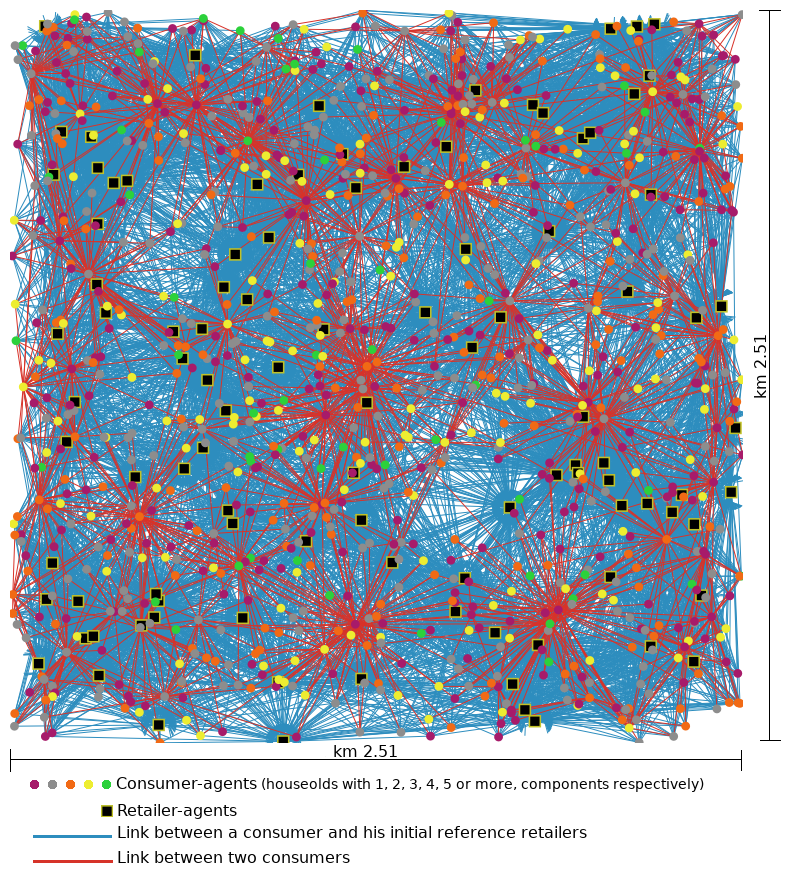
Consumer buying choices, especially in the food sector, are strongly influenced by the distance of the points of sale. Therefore, the location of the stores in relation to consumers plays an important role. In this model, it is possible to indicate the exact location of each store and each consumer family and thereby measure this distance. With this organization of data, it is possible to very precisely take into account the influence of the distance between the consumer and the different stores. Figures 1 and 2 report the agents’ locations in the applied case.
The retailer-agents
The attributes that characterize retailers in regard to consumers can be divided into structural (objective) and evocative (subjective).
Structural attributes are as follows:
- Distribution type: following the standard classification adopted by Italian statistics, this attribute can assume one of the following values: “hypermarket”, “supermarket”, “small shops with self-service”, “hard discount”, “traditional shop”, and “other” (street shops, etc.). In this model, the frequency of each distribution type follows that reached in official statistics (Appendix A - Table 1).
- Price level: this attribute assumes a numerical value, which is a multiplying coefficient (coeffpv) for the average consumer’s monthly expenditure (the average basket price) as shown in the statistics (Appendix B), so as to reproduce the variability of prices among the different shops for the same food products. The value assigned to each retailer shows how much the average level of prices charged by the retailer deviates from the average general level (which is represented by the basket expenditure collected by the statistics).
- Service level: this parameter is related to the store’s attributes, such as product information, opening hours, purchase assistance, etc.. It assumes a numerical value that represents the individual retailer’s score in the ranking lists of all retailers.
- Assortment level: this parameter summarizes characteristics such as the number of categories and brands of goods sold, and their quality (presence of fresh products and certified, branded, specialized products). It assumes a numerical value that represents the individual retailer’s score in the ranking lists of all retailers.
- Location and accessibility: this parameter depends substantially on the distance between the store and the customer’s home. Therefore, the distance between each retailer-consumer pair is considered.
- Evocative parameters are valued by each consumer subjectively (based on emotions, intuition and other personal factors) and are related to the store image, the feel (pleasantness, decor, colours), and sympathy with the clientele. Therefore, they are synthesized in a single numeric parameter that can assume different values, randomly determined, for each retailer-consumer pair.
The values of the attributes Price, Service, and Assortment level are given in Appendix A - Table 3.
The consumer-agents
The consumer-agents (families) have been segmented into five categories based on the members’ number, reflecting the frequencies of the official statistics (Appendix B - Table 7). In the model, the basic reference parameter is the average monthly expenditure for food of each family according to the number of members (Appendix B - Table 5). However, the limited product offerings of Italian FMs must also be considered. In the model, only the families’ monthly expenditure for the purchase of products usually present only in farmers’ markets is taken into consideration, as opposed to the expenditure related to all food products. It then becomes possible to compare expenditures in FMs to other types of store. Appendix C - Table 11 shows the calculation of this food basket expenditure with a further explanation.
To reproduce the variability of expenditure around the mean, determined by professional status and other factors, a random multiplicative coefficient (coeffc) was introduced, with a value between 0.8 and 1.2, which allows us to come up with a Gaussian distribution of the monthly expenditure of families around the mean. This range was calculated on the basis of the variability found in official statistics, see for example Appendix B - Table 6. In addition, to take account of the different price levels charged by shops (as discussed above), monthly expenditure is multiplied by the price level coefficient of each shop (coeffpv). The values assumed by coeffpv are reported in the column “Price Level” in Appendix C - Table 4. It follows that the price of the monthly basket is determined by the conjunction of individual consumers with individual stores. This means that it is necessary to calculate the value for every consumer-retailer pair. Therefore, in the model, the basket price is calculated with the empirical Function (1):
| $$\textit{pp}_{ij} = \textit{ppc}_i \, \textit{coeffc}_i \, \textit{coeffpv}_j$$ | (1) |
- \(\textit{pp}_{ij} =\) price of the basket purchased at the store \(j\) by the consumer \(i\);
- \(\textit{ppc}_{i} =\) price of the basket of consumer \(i\) (determined according to the number of members in the family and other parameters, see Appendix C - Table 11);
- \(\textit{coeffc}_i =\) random multiplicative coefficient of consumer \(i\);
- \(\textit{coeffpv}_j =\) multiplicative coefficient of the store \(j\).
Therefore, the Function (1) relates the consumer's expenditure for the purchase of their own food basket (parameters ppc and coeffc - see Appendix C - Table 11) with the price level characteristic of each point of sale (parameter coeffpv).
The reference points of sale
The consumer-agent buys food in the shops they prefer. The preference is formulated by taking into account at the same time the various choice criteria, which can be summarized as follows:
- the basket price, as discussed above;
- the transportation cost to reach the shop and to come back, using either the consumer’s own vehicle or public transport;
- the time spent to reach the shop and to return home and for shopping at the shop;
- the shop’s level of assortment;
- the shop’s level of service;
- other subjective or irrational factors (the “evocative” parameters).
Here, the point of sale where the basket is purchased is chosen by the consumer according to the principle of utility maximization (Lancaster 1966), which is calculated with Function (2):
| $$U_{ij} = V_j + e_{ij}$$ | (2) |
- \(U_{ij} =\) utility of the shop \(j\) perceived by the consumer \(i\);
- \(V_j =\) ``observable" component of the utility, which includes the price of the basket, the transportation cost, the cost of time spent, the level of assortment and the level of service;
- \(e_{ij} =\) ``non-observable" component of the utility, which includes subjective or irrational factors.
In the model, the component Vj was broken down into the following four parameters.
- Price of the basket, calculated using Function (1).
- Distance: this parameter is used in the model as an index of two distinct factors that affect the choice of the point of sale, i.e., the cost of transportation and time spent to do the shopping. As regards the cost of transportation, whether by personal or public transport, it is evident that the consumer makes—at least intuitively—an assessment of how much it weighs upon the total cost of products. As regards the time available for shopping, clearly the less time that is available, the more the consumer will tend to frequent the nearest shops. Therefore, by simplifying the calculation, the model uses the distance for both factors, measured between the consumer’s home and the shop.
- Level of assortment: multiplicative coefficient assigned to each shop (Appendix A —Table 4).
- Level of service: multiplicative coefficient assigned to each shop (Appendix A —Table 4).
The utility component eij represents a series of factors that are difficult to quantify, linked to the experience of each consumer, to their sensitivity and to their irrational component. Since this component is “non-observable”, it is calculated in the model through the use of a random variable that reproduces a normal statistical (Gaussian) distribution of consumer preferences. After several trials during calibration, it was decided empirically that this variable can take on values of around 0.5 with a standard deviation of 0.05.
To make the various terms of the function uniform (i.e., they can be summed together), the price of the basket and the distance are calculated to a relative degree, comparing them to the mean of the similar components of all the shops that are among the shops preferred by each consumer. Furthermore, since both the basket price and the distance are inversely proportional to utility, the reciprocal of these two factors is inserted into the calculation.
Lastly, there is the possibility of multiplying the terms of the function by a coefficient (weight) that allows us to define the relative importance; in the case of the assortment and the service level, the weight is unique. The weights are the same for all consumers; their values are chosen in the model calibration phase. Indeed, in this specific case, this possibility is not used, assigning a value of 1 to each weight.
This results in Function (3):
| $$U_{ij} = wp \frac{\sum_{k=1}^n pp_k}{n} \frac{1}{pp_{ij}} + wd \frac{\sum_{k=1}^n \textit{dist}_k}{n} \frac{1}{\textit{dist}_{ij}} + \textit{wal} \, \textit{ass}_j \, \textit{liv}_j + e_{ij}$$ | (3) |
- Uij = utility of the shop j perceived by the consumer i;
- wp = weight of the price of the basket
- n = number of points of sale taken into consideration by the consumer i
- ppk = price of the basket purchased at one of the points of sale taken into consideration by the consumer i
- ppij = price of the basket purchased at the point of sale j by the consumer i
- wd = weight of the distance
- distk = distance between the consumer i and one of the points of sale taken into consideration by the consumer
- distij = distance between the point of sale j and the consumer i
- wal = cumulative weight of the assortment and the level of service
- assj = assortment coefficient of the point of sale j
- livj= level of service coefficient of the point of sale j
- eij = “non-observable” component of the utility of the point of sale
- j perceived by the consumer i.
In the model, each consumer keeps a list of the shops that they take into consideration for shopping, the utility of which is calculated with Function (3). This list is updated continuously, introducing and removing shops on the basis of the information that reaches the consumer. For every expenditure cycle, consumers choose from their list, the points of sale they will make for the purchases of that cycle, with a preference and a probability proportional to the utility of each one.
Frequency of food shopping
Average monthly expenditure is broken down by each consumer according to shopping frequency habits, i.e., based on how many times the consumer goes grocery shopping in one month. This means that every time the consumer goes shopping, they purchase a share of their own food basket.
To understand how this expenditure is distributed among the various shops that consumers can go to in a month, in simple terms, the basket can be divided by the number of times that the consumer goes shopping in a month, assuming that each time only one shop is visited. In making this breakdown, the data in Appendix B - Table 8 have been taken into account. In any event, a certain amount of randomness is inserted in the calculation, which makes it possible to take into account two factors:
- the consumer can divide the expenditure among a different number of shops compared to what would be calculated in the manner described;
- the share of the expenditure can be different among various shops.
Points of sale actually visited
The number of points of sale actually visited may vary from one expenditure cycle to the next, and the share of the food basket purchased at each store may not follow the utility ranking that each consumer predetermines. Therefore, each consumer-agent chooses to purchase the monthly basket at a variable number of stores, both according to the number of reference stores and their utility ranking and according to other factors that are difficult to determine. These other factors are therefore defined through a probability calculation. Appendix D contains the pseudocode of the retailer-choosing algorithm and a further discussion.
Information on the points of sale
The model considers two methods for consumers to acquire information on shops: word of mouth and “short range” advertising. In addition to the list of “reference” shops, at which the consumers normally may make purchases, every consumer keeps a list of outlets “to check out” that includes the points of sale suggested either by word of mouth or through advertising. With every buying cycle, the consumer has a certain probability of trying one or more of the shops on the “to check out” list, in addition to those on the reference list. This takes into account inertia in changing buying habits, which for most food consumers is usually strong.
The model implemented the creation of a network among consumers, each of whom is connected with a certain number of other consumers. The network responds to the particular characteristics of consumer networks: i.e., a high clustering coefficient, a distribution of the links of each consumer (degrees) corresponding to the scale-free characteristic and a fairly small average diameter.
This network is also defined within a real geographic space, i.e., that defined by the position of the points of sale, by that of the consumers and by the road graph that connects them. This takes into account the fact that the closer people are to each other physically, the more they tend to establish ties. The existing links in the network at any time allow the consumer-agents to share their opinions about the stores they know (thanks to word of mouth), so that they may consider visiting stores other than the usual ones. Appendix E contains the pseudocode of the word-of-mouth algorithm and further discussion.
“Short-range” advertising is understood as all forms of advertising that can be carried out at a local level, to inform or remind the consumer about the existence and the characteristics of a certain shop (posters, flyers, commercials on local radio and TV, ads in local newspapers, etc.). While word of mouth is a source of information that is always active, given that consumers are able to exchange views with each other at any time, advertising works for a well-defined period of time, corresponding to the length of the advertising campaign. Therefore, a simple algorithm was implemented in the model that can be activated “by request,” for example when a new store opens. Appendix F contains the pseudocode of the short-range advertising algorithm and a further discussion.
Parameter values of each consumer-agent
On the basis of these arguments, the attributes for each consumer-agent have been defined as follows.
- Family size, variable from 1 to 5 or more members.
- Multiplying coefficient for the customization of the family’s basket price (a random value ranging from 0.8 to 1.2).
- Expenditure frequency, i.e., the number of days in a month the consumer goes shopping. It can take these values: 26 (daily expenditure), 5 (weekly), 3 (every 10–15 days), 1 (monthly). This value is used in the probabilistic calculation of the number of shops actually visited in a month, based on real statistical data (Appendix B —Table 8).
- Average number of visited shops, ranging from 1 to 9. This value is also used in the probabilistic calculation of the number of shops actually visited in the month. The frequency distribution of the average number of visited shops, within the population of consumer-agents, reflects that found in one of the few such published studies (Appendix B —Table 9).
- List of reference shops, each with these personal attributes:
- customized basket price, calculated by Function (1);
- “non-observable” utility component, a normally distributed random floating point number, with average value = 0.5 and standard deviation = 0.05;
- total consumer utility to the shop, calculated by Function (3).
- List of shops to be checked, each with this attribute:
- verification urgency, an integer number equal to the number of network friends who recommended that shop (see Appendix E for further explanation).
Model Operation
Starting environment
The model acts in a predefined environment that reproduces, in relation to the retail food market, the average Italian population and distribution frequencies. This environment is made up of 1,000 consumer-agents and 103 food-store agents. In order to avoid weighing down the model with a high number of agents, it has been assumed that each consumer agent represents 10 families. Since a family has an average number of members equal to 2.4 (ISTAT 2014), the model represents a population of 24,000 inhabitants. In relation to this number of inhabitants, in Italy there are on average 103 grocery stores, broken down by distribution type as shown in Appendix C — Table 10. Each agent has its own fixed location, on the basis of which mutual distances are calculated. The territorial distribution of consumers reflects that of a medium-sized city in central Italy; considering an average density of 3,800 inhabitants per km2 (our ISTAT 2014 data processing), the geographical area taken into consideration in the model is about 6.3 km2.
The environment also consists of two networks. The first network is the relational network that interconnects the consumers. Each consumer-agent has a number of “friends”, which depends on chance, but the network as a whole reflects the characteristics illustrated above. The second network connects each consumer with his or her starting reference stores, which simply are the 10 closest retailers. Figure 1 shows this starting environment.
Model operation details
The model was run on the environment described above, observing the evolution of the system. Only the consumers had dynamic behaviour, as each of them carried out a reference stores’ utility assessment and amended the list using the information obtained from other consumers, thanks to word of mouth. The model operation was divided into two steps: the first was the market adjustment phase, which led to a market equilibrium; the second started with the FM opening, which led to a new and different market equilibrium.
Consumers had two basic capabilities in their spending behaviour:
- to continuously adapt to market changes, reconsidering their preferences;
- to gather information on retailers and change their preferences; this information arises from two sources: the word of mouth within the consumer’s social network and the advertising optionally carried out by retailers.
The model dealt essentially with the following functions:
- average monthly expenditure of each family-agent for the foods considered;
- how the flow of information on retailers occurs and the effects it had;
- how many and which retailers were selected for each shopping trip;
- how the average monthly expenditure was distributed among the retailers visited.
Each family had a list of reference retailers and each time decided which stores to shop at, on the basis of a utility function that considers the price level of each retailer, the distance, and the structural and evocative characteristics described above. Each family, for each buying cycle, decided according to its behavioural characteristics how to divide the food expenditure among the reference retailers. The list of reference stores was the subject of ongoing audits and possible changes, according to the influence of word of mouth and advertising.
Step 1 of the model operation: market adjustment phase
Starting from the initial set-up of the model, in which the list of reference stores included just the nearest 10 stores (the authors’ choice, based on the assumption that consumer’s will initially consider only the nearest stores), the consumer-agents assess all the other shops that might be of interest, changing the initial preference ranking and arriving at a new ranking, which does not change until the offer of stores changes. At the end of this phase, the market stabilizes, reproducing a market equilibrium by retail type (Table 2) and the consumer-agent tended to always shop in the same stores, apart from fluctuations due to the randomness of purchase at every shopping cycle.
The purchasing behaviour of all the families in the area made it possible to determine a certain distribution of revenue among retailers. More specifically, the model reproduces a typical Italian distribution of revenues among the various types of food retailers: the largest share of revenues being held by a small number of big stores (supermarkets and hypermarkets), while a considerably smaller share is held by a large number of small traditional food shops, and the lowest shares by other types of retailers (self-service shops, hard discount, etc.). At this point, each store has conquered its own market share, which it maintains indefinitely, since there are no events capable of disturbing the achieved equilibrium and consumer demand is constant. Thus, a typical oligopolistic, non-collusive Nash equilibrium is reached. As long as there are no perturbative action, the equilibrium remained, with normal oscillations that did not affect the average general equilibrium.
Appendix G further describes this first step. Table 2 compares the statistical data on revenue quotas by distribution type with the model data at equilibrium achieved (in the model, hypermarket and supermarket typologies are united). There was substantial closeness of data. The differences between statistical and model data was probably due to the fact that the number of shops in each type of model had necessarily to be a whole number, while in real statistics the number was decimal (see Appendix C - —Table 8); for example, in relation to the number of inhabitants of the model, supermarkets and hypermarkets should be 3.71; in the model they are rounded to 4, so an increase of 0.29 can have a great effect, as it is the dominant type.
| Type | Statistical data, Italy, 2012 (FederDistribuzione 2012) | Data obtained by the model* (averages of 20 repetitions between tick 400 and 499) |
| Hypermarkets | 11.5% | 53.5% (1.02) |
| Supermarkets | 40.6% | |
| Small stores with self service | 9.4% | 7.7% (0.49) |
| Hard discounts | 10.5% | 11.9% (0.78) |
| Traditional shops | 17.9% | 15.6% (0.49) |
| Street shops and other | 10.1% | 11.3% (0.41) |
| Total | 100.0% | 100.0% |
In order to assess the stability of the model, 20 repetitions were performed. In each repetition, the positions of agents and the starting links between them were constant (Figure 1). On the other hand, the rating of the stores by each consumer agent were able to change in each tick, changing the order of preference according to the utility calculation made according to Function 3. Table 2 data confirmed the stability of the model, which was able to reproduce the same trend in all 20 repetitions with very low variability.
Step 2 of the model operation: FM opening
In the equilibrium situation, at the time and place chosen by the operator, a FM was opened through the creation of a new retailer-agent, to which the values of the specific FM attributes were assigned.
Introducing the farmers’ market topic, one can tackle other issues of consumer behaviour relating, for example, the reasons and means of consuming fresh fruit and vegetables and the ascertainment of methods by which they are produced. These issues are strictly related to the notion of sustainable consumption. This study considered the monthly expenditure of families to purchase a basket of those food items that are normally found at an Italian farmers’ market, rather than that regarding the purchase of all food items. It was therefore possible to compare the expense at FMs and other types of retailers on the basis of the same basket of foodstuffs.
The opening of the FM caused a disequilibrium in the market. Gradually but increasingly, consumers discovered the existence of the new shop and visited it. The output of the model made it possible to check the evolution of the performance of the new FM. As time went by, a new equilibrium was created, where one could check the new shop ranking (in terms of the number, type and origin of the customers and in terms of revenue).
The model simulation was replicated 20 times using the same initial parameters. In each repetition, a single FM was opened at the 500th cycle and the simulation was allowed to proceed at least to the 1,500th cycle. The location of the FM was changed each time, allowing an evaluation of the economic results in each location. By the 1,500th cycle, an equilibrium in terms of share of the revenue had been recreated.
Figure 2 shows the 20 investigated locations.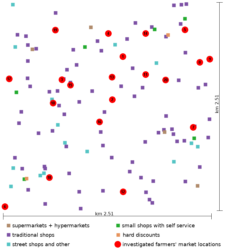
Results
Best location of the new FM and changes at the revenue level
As expected, the share of revenue reached by the FM was different for each replication, due to the different locations. In order to ensure the survival of the new small FM, the best location is where it could have the highest revenue level.
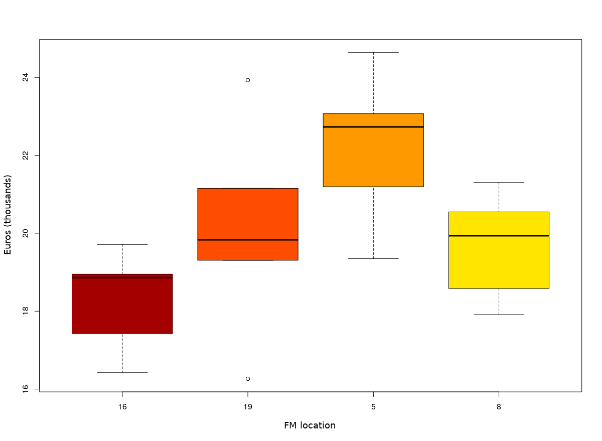
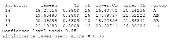
By analysing with ANOVA the average revenue of the FM between cycles 1,400 and 1,499 in each of the 20 repetitions, we can extrapolate that location 5 (Figure 2) was probably the best, with a mean revenue level of 23,067 Euros per cycle (see Appendix H for detailed ANOVA output). To confirm this result, an additional four repetitions were performed for each of the four best locations identified in the previous analysis (locations 5, 8, 16, and 19). The output of the ANOVA confirms that location 5 retains a statistical advantage over other positions (Appendix I), as shown in Figure 3.
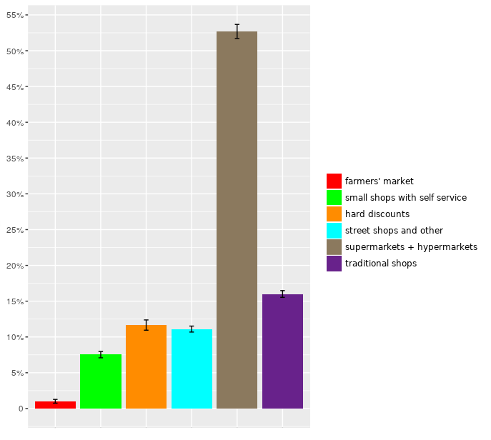
The average revenues above represented 1.01% of the average total revenue for the considered food basket (Figure 4). Because there is little data on the level of FMs’ revenues in Italy, for a very general comparison with real data it is only possible to mention three cases. Regarding the covered market in Montevarchi, which is a daily FM that first opened in February 2008, a monthly revenue of 90,000 Euros was recorded in November 2008, along with an incidence of 2.0% of purchases for the food expenditure of families in Montevarchi (Filippini and Zucconi 2009). Regarding two other Italian FMs, located in Vetralla and in San Giovanni Val d’Arno, the monthly revenues in 2010 was 12,500 Euros and 13,300 Euros, respectively (Marino et al. 2012). Thus, the average level of revenue reached by the FM activated in the model was compatible with that reported in the few cases cited in the literature.
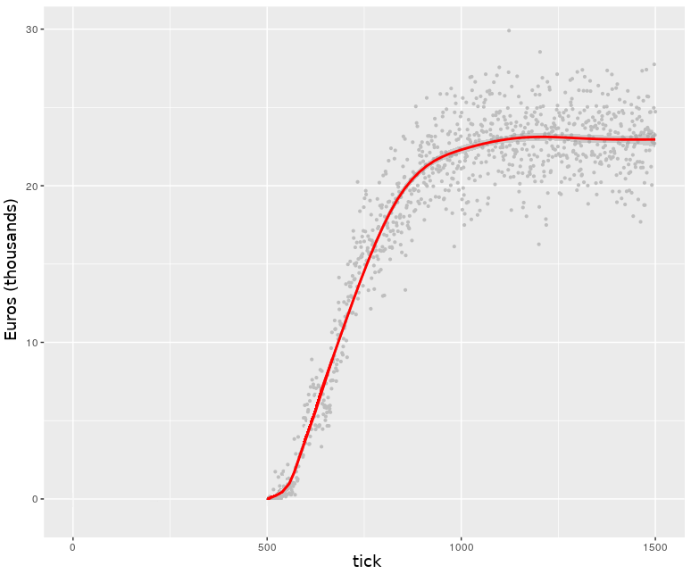
The revenue growth curve
A further note on the results was the trend of FM revenue growth. The graph of revenue growth (Figure 5) follows an S-curve, in which the growth is exponential at first, then becomes logarithmic and finally stabilizes with no further growth. This curve is typical of the Bass model (Bass 1969) for the diffusion of innovation. A similar trend is often seen in agent-based models dealing with this topic (Kuandykov and Sokolov 2010; Kiesling et al. 2012).
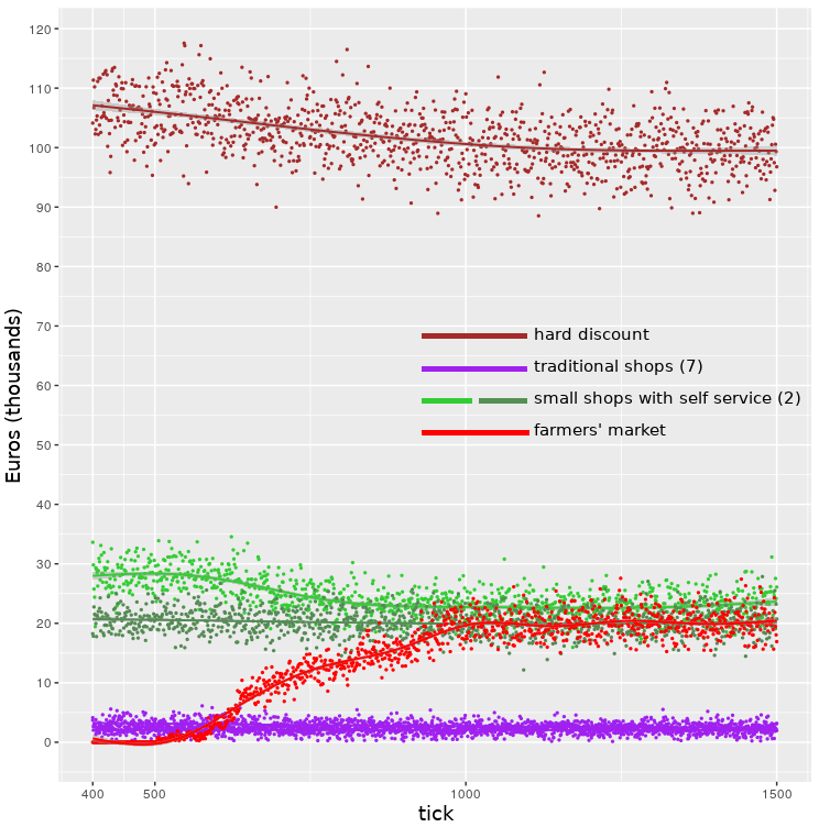
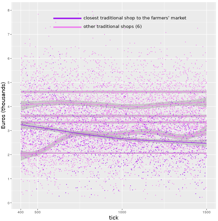
Competition with closest retailers
In this model, it is assumed that total food expenditure does not change with the FM opening. It therefore follows that some retailers see their revenues falling. Figure 6 and Figure 7 show the revenue trend of the 10 stores closest to the FM (one hard discount, two small stores with self-service, and seven traditional stores). We can notice a revenue decrease for hard discount, for the closest small store with self-service and for the closest traditional store, while the others maintain unchanged revenue. It is clear that the high level of service of the traditional shops makes them able to withstand the new FM, except for the closest one, while for the hard discount and for the closer small store with self-service, the opening of a store with better quality becomes an important direct competitor. This result is consistent with research that has highlighted the impact of FM on consumers’ buying habits, with a shift towards the purchase of fresher products (as in Widener et al. 2013).
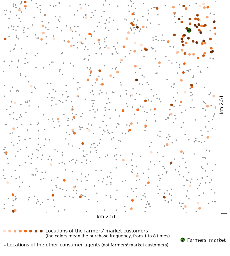
Customers’ number and location
The simulation also provided a result regarding the average number of FM customers per cycle once equilibrium was reached. The average for the 20 repetitions was 81.96 consumer-agents, corresponding to 819.6 families (8.2% of the total).
The total number of customers (i.e., families) of all shops was on average 39,291.7. As the model comprised 10,000 families, this means that each family in each cycle purchases on average in 3.93 shops and that the number of FM customers represents on average 2.09% of all food store customers.
Figure 8 shows the location of FM customers in the last eight ticks and their purchase frequency. It is clear that the most numerous and frequent customers were also the closest to the FM, but it is also noticeable that there are many more distant customers.
Characteristics of FM customers
With an in-depth analysis of the model’s results, it was possible to highlight the characteristics of families who made purchases in the FM.
- The family was slightly larger, but does not appear to be significantly so: 2.47 members in the families buying in the FM against 2.38 members as a general average (3.6% more).
- The families buying in the FM do their shopping more frequently (17.9 times in a month) than the general average (10.3 times in a month) and visit more shops (5.7 versus 4.1).
- To purchase the monthly basket considered here, the families spent on average as much as the other families (158.8 Euros versus 159.3, respectively). Since they visit more shops, this meant that they spent less on average in each one.
- The families buying in the FM travel for food shopped at a much greater distance than the customers of traditional shops (801 meters against 89) and a shorter distance than the customers of hard discounts (1,209 m), supermarkets and hypermarkets (1,217 m), and small shops with self-service (965 m). They travelled almost the same distance as the customers of street shops and other (747 m).
Characteristics of the customers’ social network
The network creation algorithm in the model allowed the reproduction of three basic characteristics that the literature reports for social networks:
- high clustering coefficient: the 20 replications had an average coefficient of 0.52;
- small diameter: the 20 replications had an average diameter of 3.8;
- scale-free: the distribution of the links respects this characteristic (Figure 9).

Discussion and Conclusions
The ABM method has made it possible to develop a model that imitates the consumer’s decision-making process and the diffusion of innovation in the food market. This takes into account the spatial components of these processes, namely the location of the various players. The model showed that it is able to reproduce some of the real market dynamics, including the division of market share among the various types of food retailers and calculating the market share of a new, small food retail shop.
The case examined here, involving the opening of a small-sized FM, made it possible to test the behaviour of the model in a more specific context, analysing the placement of the new shop in a local market and observing the evolution of this market caused by the new shop’s opening. As a result, we can estimate how many families will change their consumption habits, switching to a more sustainable consumption, also predicting the economic positioning and the best location of a new FM, namely where it can get the highest revenue. This information is crucial to the survival of a new, small shop.
Specifically, the results of the simulation highlighted certain aspects that seem very interesting.
First of all, the great effectiveness of word-of-mouth needs to be underlined. This, together with a short advertising campaign in the simulation, allowed the new FM to have an adequate number of customers in a short time. The intention of the model was not to define the timing of events precisely but, considering that the exchange of information among the consumers due to word-of-mouth could have taken place on a daily basis and that therefore the duration of the tick could be one day, it can be said that the FM reached its full revenue in one and a half years (about 550 days; see Figure 5).
Of the 20 FM locations examined, location 5 was the best in terms of achievable revenue. This location was somewhat decentralised with respect to the geographical area examined (Figure 2), so it seems that the FM location is not so important. Indeed, FM customers travelled a rather long distance to reach it, despite the fact that it has a smaller variety of food on offer than other types of shops. The long distance travelled, combined with the higher number of shops visited and the higher frequency of shopping (compared to the overall average), indicate that the FM customers spend more time on shopping than the other customers. But at the same time they do not spend more money than the other families. It is clear therefore, that an increased spread of FMs would allow access to FMs for a much larger number of families, i.e., even those who have less time to spend for shopping, but without increasing the price levels. This result is consistent with what was reported by Widener et al. (2013) (see Table 1) and seems applicable to all the types of food shops that focus on the supply of local and fresh products, contributing to the idea of sustainable consumption.
Lastly, the model results also indicate that the opening of just one FM had a major impact on consumer behaviour, as 8.2% of the families purchased at least once in the FM, changing, more or less, their dietary habits.
As concerns some general objectives, the study pointed out the feasibility of using an ABM even in a complex food supply chain, such as the Italian one. Here, the need to consider a large number of variables makes the use of this method, created precisely to consider a large variety of agents and behaviour, even more attractive. It is clear that being able to consider all variables implies a big job of further in-depth investigation and processing, which was not possible in this study. The work however, has made it possible to highlight certain key issues, which can be considered in any future development.
Acknowledgements
This research derives solely from the interest of the authors and did not receive any specific grant from funding agencies in the public, commercial, or not-for-profit sectors.Appendix
A
| Type | Number | Incidence rate | Stores per 100,000 inhabitants |
| traditional food stores | 189,238 | 74.21% | 317.06 |
| street shops and other | 36,878 | 14.46% | 61.79 |
| small with self-service | 15,128 | 5.93% | 25.35 |
| supermarket | 8,823 | 3.46% | 14.78 |
| hard discount | 4,560 | 1.79% | 7.64 |
| hypermarket | 393 | 0.15% | 0.66 |
| Total | 255,020 | 100.00% | 427.28 |
| Type | Price level | Assortment level | Service level |
| traditional food stores | 1.15 | 0.92 | 1.10 |
| street shops and other | 1.00 | 0.90 | 1.10 |
| small stores with self-service | 1.05 | 1.00 | 1.07 |
| supermarkets and hypermarkets | 1.05 | 1.10 | 1.06 |
| hard discounts | 0.90 | 1.00 | 0.96 |
| farmers’ markets | 1.00 | 0.92 | 1.10 |
In the current study phase, which assumes a theoretical connotation in that a hypothetical territorial case is analysed, in assigning a value to the attributes it has been considered that it is possible to refer to the retailer’s distribution type, assigning identical values to all the shops of the same type. It is clear that this method of assigning values is a simplification, due to the lack of data collected on the ground. Obviously, in a real application of the model, it will be possible to carry out a specific survey to better determine the value of these parameters for each retailer.
The values of the parameters reported in this table have been elaborated by interviewing some experts in the food supply chain and in food retailing particularly. It is believed that these values are realistic as they allow to reproduce the real market shares of the different retailer’s distribution types, as ascertained by statistical surveys (see Table 2).
B—Statistical data
| Number of members | Amount (Euros) |
| 1 | 332.65 |
| 2 | 468.17 |
| 3 | 536.29 |
| 4 | 585.76 |
| 5 or more | 663.77 |
| Overall average | 468.32 |
| Professional status | Amount (Euros) |
| entrepreneur or freelancer | 521.05 |
| self-employed worker | 493.86 |
| executive or employee | 503.37 |
| worker or equivalent | 490.35 |
| retired | 444.33 |
| unemployed, housewife, etc. | 407.92 |
| overall average | 468.32 |
| Number of members | Frequency |
| 1 | 31.1% |
| 2 | 27.1% |
| 3 | 19.9% |
| 4 | 16.2% |
| 5 or more | 5.7% |
| Total | 100.0% |
| Frequency | Number of family members | ||
| 1 | 2 | 3 or more | |
| daily | 25.8% | 18.3% | 28.9% |
| weekly | 57.7% | 65.6% | 58.9% |
| every 10–15 days | 11.8% | 13.7% | 9.5% |
| monthly or less | 4.7% | 2.4% | 2.7% |
| Total | 100.0% | 100.0% | 100.0% |
| No. of visited shops | Frequency |
| 1 | 4.08% |
| 2 | 18.21% |
| 3 | 22.28% |
| 4 | 20.11% |
| 5 | 14.95% |
| 6 | 13.04% |
| 7 | 4.89% |
| 8 | 1.90% |
| 9 | 0.54% |
| Total | 100.0% |
C—Model implementation
| Type | Statistical data (see Table 3 above) | Data implemented in the model stores per 24,000 inhabitants* | |||
| Stores per 100,000 inhabitants | Stores per 24,000 inhabitants | Incidence rate | Number | Incidence rate | |
| traditional stores | 317.06 | 76.09 | 74.21% | 76 | 73.79% |
| street shops and other | 61.79 | 14.83 | 14.46% | 15 | 14.56% |
| small stores with self-service | 25.35 | 6.08 | 5.93% | 6 | 5.83% |
| supermarkets + hypermarkets | 15.44 | 3.71 | 3.61% | 4 | 3.88% |
| hard discounts | 7.64 | 1.83 | 1.79% | 2 | 1.94% |
| Total | 427.28 | 102.54 | 100.00% | 103 | 100.00% |
| Type | Number of Family Members | Average | ||||
| 1 | 2 | 3 | 4 | 5 or more | ||
| confectionery | 7,71 | 12,17 | 14,56 | 16,35 | 17,67 | 12,21 |
| cheeses | 19,54 | 29,46 | 32,04 | 34,57 | 37,29 | 28,08 |
| eggs | 4,22 | 5,61 | 6,29 | 7,18 | 8,69 | 5,73 |
| olive oil | 9,54 | 12,64 | 11,93 | 12,22 | 13,67 | 11,51 |
| fresh vegetables and fruit | 63,16 | 86,91 | 93,69 | 97,25 | 107,19 | 83,48 |
| wine | 8,82 | 14,62 | 13,24 | 12,43 | 11,88 | 12,01 |
| Total FM basket | 112,99 | 161,41 | 171,75 | 180 | 196,39 | 153,02 |
Every family has a fairly constant demand for food products (see Table 1 above). Within this demand, there is a basket of products that are normally sold in FMs and that can be found as the same or similar products in the other types of shops. The basket of food products sold in the Italian FM, to some extent, can be defined by these types of products:
- fresh vegetables and fruit,
- eggs,
- cheeses,
- olive oil,
- wine,
- confectionery.
The average expenditure, which we have defined as “FM basket”, for each of these product types is reported disaggregated in the official statistics (ISTAT 2012). In addition, a further breakdown by the number of household members is available. In the application case of the model, therefore, the monthly expenditure of households for the purchase of the FM basket is considered, rather than the purchase of all food products, so that it is possible to make a comparison between the expenditure in FMs and in the other types of stores, based on the same basket of food products.
The values of Total FM basket, shown in this table, are used in the ppc parameter of the Function (1).
D—Algorithm 1
Purpose
For the current shopping cycle, each consumer chooses the shops to visit and the expenditure quota for each shop.
Rationale
Choosing the shops for a shopping cycle, the consumer applies his or her own utility calculation. At each purchase cycle, the consumer chooses a number of shops that are part of the list of reference shops; this number is determined by shopping habits, in the sense that it is likely to increase as the number of shops the consumer visits on average increases and the frequency of shopping increases. Once it has been established which stores are taken into account for the current purchase cycle, the share of the expenditure reserved for each is calculated, with decreasing probability as the utility of each point of sale decreases; this means that the distribution of the expenditure share is subject to a probability calculation, i.e., the first store (the one with the highest utility) has a higher probability of having the largest share of the expenditure, but not the certainty.
Variables
- reference_shops: shops that each consumer considers for shopping; this list can change at every shopping cycle, because of the word of mouth or the self-finding.
- max_number_of_shops_to_visit: maximum number of shops visited at every shopping cycle; this is set in the model set-up phase, with a different and casual value for each consumer, ranging from 1 to 10.
- basket_price: total expenditure for the monthly food basket purchased by each consumer; this is determined by the conjunction of the individual consumer with the individual shop; this means that its value is different for every consumer-shop pair.
Pseudocode
E—Algorithm 2
Purpose
Thanks to word of mouth, a consumer has the opportunity to add other shops to his or her list of shops to be checked.
Rationale
Communication only takes place between consumers who are directly linked and can take place in both directions; in any case, communication takes place only if a probability threshold is exceeded.
The communication concerns the existence of one or more stores that are not included in the list of the consumer’s reference stores. If there is communication between a consumer and his or her friend, they check the respective lists of reference shops; if there are different shops, the consumer can add the new ones to the list of stores to be checked. However, the addition of new stores is subject to an additional threshold of probability, decreasing from the first to the last addable store, since the stores are ordered by decreasing utility; this is because it is supposed that each friend is more stimulated to communicate, among his or her reference stores, those that have greater utility for that individual; therefore the algorithm has been built in such a way that passing from one store “communicable” to the next (which has a lesser usefulness) the probability of addition decreases. Each store included in the “to be checked” list is given an “urgency of verification” variable; each time another consumer suggests a store that is already in the “to be checked” list, the value of this variable is increased. Stores with higher “urgency” are more likely to be considered for inclusion in the list of reference shops. In this way, a kind of “social pressure” can be created that directs the consumer towards certain shops. As we can see, the algorithm implemented distinguishes between two possibilities: that of considering a store (list “to be verified”) and that of actually using it for purchases (“reference” list). In this way, an account is taken of the inertia in changing purchasing habits, where most food consumers change their buying habits with a certain degree of difficulty. When one of the shops to be checked is considered for purchase, it becomes part of the reference list.
Variables
friend_reference_shops: list of friend’s reference shops
coefficient_of_decrease: takes the value of 0.8
Pseudocode
F—Algorithm 3
Purpose
On opening, the FM launches a short-range advertising campaign, reaching a share of consumers in the area
Rationale
The algorithm acts by soliciting a number of consumers to the store being advertised, i.e., by including the store in the “to be checked” list of those consumers. Each of them is chosen when a certain threshold of probability of being reached by the advertising message is exceeded; the probability increases as the distance between the consumer and the store decreases, as it is believed that the consumer is more interested, and therefore more attentive to the advertising message, the closer the store is.
Variables
probability_threshold: takes the initial value of 0.5
this_shop: shop that launches the advertising
Pseudocode
set consumers_list = random quota of all consumers
order consumers_list by increasing distance from this_shop
set reduction = probability_threshold / consumers_list_length
repeat for each consumer in consumer_list
	set probability1 = random number ranging from 0 to 1
	if probability1  < probability_threshold
		add this_shop to the list_of_shops_to_be_checked
		set this_shop_urgency = 1
	end if
	set probability_threshold = probability_threshold - reduction
end repeat for each
G
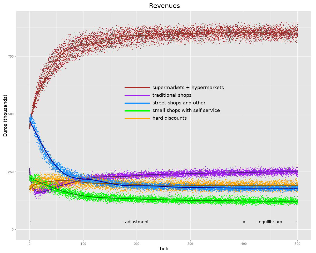
Figure 10 shows the trend in revenue of the different types of retailers since the start of the model’s operation. Cloud points indicate revenue at each tick in each of the 20 repetitions and the lines indicate the trend. Actually, the operating phase we are interested in is the one that starts around tick 400, when the market stabilizes, maintaining an equilibrium until an event capable of disturbing the market happens, such as the opening of the FM at tick 500. In this equilibrium phase, a distribution of revenue is reached that is very similar to that shown by official Italian statistics, so we can say that the model is representative of the situation in the Italian market. Although the phase prior to tick 400 is only an adaptation phase, it is still possible to have interesting indications that confirm the validity of the model, as discussed hereafter.
<At the time of the initial set-up of the model, just as a choice of ours for the starting environment, the list of the reference shops of each consumer contains only the 10 stores closest to him or her, therefore with a probability of containing traditional shops, which is by far the most represented type, much greater than the other types of shops (see Table 6 above). As the consumer progresses with the evaluation of other stores, market shares gradually shift from traditional shops and other types of stores to supermarkets and hypermarkets.
In the very early stages of the model’s operation, street shops and others have a very high share of revenue because, although they are fewer than traditional shops, they have a lower price level that makes them very competitive with neighbouring consumers.
It can also be noted that at first the revenue of traditional shops is rapidly decreasing, but then slowly it increases, almost reaching the starting level; this trend is an indication of the fact that initially many consumers move towards other types of cheaper retailers, but then a group of consumers is formed that is narrower but willing to pay more to have a better and more personalized level of service and also willing to travel longer distances to achieve this goal.
The evolution represented by Figure 10 is comparable to that in Italy and other countries in recent decades, with a huge increase in the importance of supermarkets, to the detriment of the other types.
H—ANOVA output

Appendix I—ANOVA output
References
AKERLOF, G. A. (1970). QUALITY UNCERTAINTY AND THE. The quarterly journal of economics, 84(3), 488-500.
ANNUNZIATA, A., & Scarpato, D. (2014). Factors affecting consumer attitudes towards food products with sustainable attributes. Agricultural Economics/Zemedelska Ekonomika, 60(8).
AUCHINCLOSS, A. H., Riolo, R. L., Brown, D. G., Cook, J., & Roux, A. V. D. (2011). An agent-based model of income inequalities in diet in the context of residential segregation. American journal of preventive medicine, 40(3), 303-311.
BASS, F. M. (1969). A new product growth for model consumer durables. Management science, 15(5), 215-227.
BERGER, T. (2001). Agent‐based spatial models applied to agriculture: a simulation tool for technology diffusion, resource use changes and policy analysis. Agricultural economics, 25(2‐3), 245-260.
BORRAZ, F., Dubra, J., Ferrés, D., & Zipitría, L. (2014). Supermarket entry and the survival of small stores. Review of Industrial Organization, 44(1), 73-93.
BRUNORI, G., & Lari, A. (2012). Strategie per il consumo sostenibile: dall’efficienza alla sufficienza.
BUURMA, J., Hennen, W., & Verwaart, T. (2017). How social unrest started innovations in a food supply chain. Journal of Artificial Societies and Social Simulation, 20(1).
CASSIA, F., Ugolini, M., Bonfanti, A., & Cappellari, C. (2012). The perceptions of Italian farmers’ market shoppers and strategic directions for customer-company-territory interaction (CCTI). Procedia-Social and Behavioral Sciences, 58, 1008-1017.
CENSIS (2010). CENSIS Note & Commenti – Le abitudini alimentari degli italiani. No. 7/8
DYER, G. A., & Taylor, J. E. (2011). The corn price surge: impacts on rural Mexico. World Development, 39(10), 1878-1887.
FEAGAN, R. B., & Morris, D. (2009). Consumer quest for embeddedness: a case study of the Brantford Farmers' Market. International Journal of Consumer Studies, 33(3), 235-243.
Federdistribuzione (2012). Mappa del sistema distributivo italiano. https://www.federdistribuzione.it
FIELKE, S. J., & Bardsley, D. K. (2013). South Australian farmers’ markets: tools for enhancing the multifunctionality of Australian agriculture. GeoJournal, 78(5), 759-776.
FILIPPINI, R. & Zucconi, S. (2009). La vendita diretta in Lombardia. Bologna: Nomisma
FRANCIS, M., & Griffith, L. (2011). The Meaning and Design of Farmers’ Markets as Public Space An Issue-Based Case Study. Landscape Journal, 30(2), 261-279.
FRANCO Silvio, Cicatiello Clara (2013). I consumatori delle Filiere Corte: tratti comuni e specificità. Workshop “Le filiere corte nella nuova dinamica città/campagna” - May 29, 2013, Roma
MARINO, D., & Franco, S. (2012). Il mercato della Filiera corta I farmers’ market come luogo di incontro di produttori e consumatori.
GAGLIARDI, D., Niglia, F., & Battistella, C. (2014). Evaluation and design of innovation policies in the agro-food sector: An application of multilevel self-regulating agents. Technological Forecasting and Social Change, 85, 40-57.
GIARÈ, F., & Giuca, S. (2012). Agricoltori e filiera corta: profili giuridici e dinamiche socio-economiche.
GORYNSKA-GOLDMANN, E., Adamczyk, G., & Gazdecki, M. (2016). Awareness of sustainable consumption and its implications for the selection of food products. Journal of Agribusiness and Rural Development, (3 [41]).
HAPPE, K., Kellermann, K., & Balmann, A. (2006). Agent-based analysis of agricultural policies: an illustration of the agricultural policy simulator AgriPoliS, its adaptation and behavior. Ecology and Society, 11(1).
ISTAT (2012). Average monthly expenditure. http://dati.istat.it/Index.aspx?DataSetCode=DCCV_SPEMMFAM
ISTAT (2014). Annuario statistico italiano 2014. Chapter 3: Popolazione e famiglie
KAYE-BLAKE, W., Schilling, C., & Post, E. (2014). Validation of an agricultural MAS for Southland, New Zealand. Journal of Artificial Societies and Social Simulation, 17(4), 5.
KIESLING, E., Günther, M., Stummer, C., & Wakolbinger, L. M. (2012). Agent-based simulation of innovation diffusion: a review. Central European Journal of Operations Research, 20(2), 183-230.
KREJCI, C., & Beamon, B. (2015). Impacts of farmer coordination decisions on food supply chain structure. Journal of Artificial Societies and Social Simulation, 18(2), 19.
KUANDYKOV, L., & Sokolov, M. (2010). Impact of social neighborhood on diffusion of innovation S-curve. Decision Support Systems, 48(4), 531-535.
LANCASTER, K. J. (1966). A new approach to consumer theory. Journal of political economy, 74(2), 132-157.
LASSAR, W. M., Manolis, C., & Lassar, S. S. (2005). The relationship between consumer innovativeness, personal characteristics, and online banking adoption. International Journal of Bank Marketing, 23(2), 176-199.
MÄGI, A. (1999). Store loyalty? An empirical study of grocery shopping. Economic Research Institute, Stockholm School of Economics (EFI).
MANCINI, P., Marchini, A., & Simeone, M. (2016). Eating Behaviour and Well-being: An Analysis on the Aspects of Italian Daily Life. Agriculture and Agricultural Science Procedia, 8, 228-235.
MARCHINI, A., Diotallevi, F., Paffarini, C., Stasi, A., & Baselice, A. (2015). Visualization and purchase: an analysis of the Italian olive oil grocery shelves through an in-situ visual marketing approach. Qualitative Market Research: An International Journal, 18(3), 346-361.
MARINO, D., Cicatiello, C., Franco, S., Pancino, B., Mastronardi, L., & De Gregorio, D. (2012). Una prima valutazione degli impatti dei farmers’ market in Italia.
MCPHEE-KNOWLES, S. (2015). Growing food safety from the bottom up: An agent-based model of food safety inspections. Journal of Artificial Societies and Social Simulation, 18(2), 9.
MIKKOLA, M. (2015). Business concept as a relational message: supermarket vs independent grocery as competitors for sustainability. International Journal on Food System Dynamics, 6(4), 225-235.
NASH, J. (1951). Non-cooperative games. Annals of Mathematics, (pp. 286–295)
NAZRUL Shaikh, N. I., Rangaswamy, A., & Balakrishnan, A. (2010). Modeling the diffusion of innovations through small-world networks.
NILSSEN, T. (1992). Two kinds of consumer switching costs. The RAND Journal of Economics, 579-589.
ROVAI, M., Fastelli, L., & Pucci, F. (2013). Verso una pianificazione efficace delle aree agricole periurbane: un nuovo approccio metodologico per la Piana di Lucca. In XXXIV Conferenza Aisre.
SADLER, R. C. (2016). Strengthening the core, improving access: Bringing healthy food downtown via a farmers' market move. Applied Geography, 67, 119-128.
SAQALLI Saqalli, M., Gérard, B., Bielders, C. L., & Defourny, P. (2011). Targeting rural development interventions: Empirical agent-based modeling in Nigerien villages. Agricultural Systems, 104(4), 354-364.
SCHENK, T. A., Löffler, G., & Rauh, J. (2007). Agent-based simulation of consumer behavior in grocery shopping on a regional level. Journal of Business Research, 60(8), 894-903.
TOLBA, A. (2007, September). Scale free networks; a literature review. In Proceedings of the International Conference on Complex Systems.
TRAVERS, J., & Milgram, S. (1977). An experimental study of the small world problem. In Social Networks (pp. 179-197).
VARIAN, H. (1992). Chapter 24, Externalities” and “Chapter 25, Information” in Microeconomic Analysis.
VERAIN, M. C., Dagevos, H., & Antonides, G. (2015). Sustainable food consumption. Product choice or curtailment?. Appetite, 91, 375-384.
WANG, H., Qiu, F., & Swallow, B. (2014). Can community gardens and farmers' markets relieve food desert problems? A study of Edmonton, Canada. Applied Geography, 55, 127-137.
WATTS, D. J., & Strogatz, S. H. (1998). Collective dynamics of ‘small-world’networks. Nature, 393(6684), 440.
WIDENER, M. J., Metcalf, S. S., & Bar-Yam, Y. (2013). Agent-based modeling of policies to improve urban food access for low-income populations. Applied Geography, 40, 1-10.
WILENSKY, U. (1999). Center for connected learning and computer-based modeling. In Netlogo. Northwestern University. http://ccl.northwestern.edu/netlogo.