
Introduction
In recent years, sport and leisure activities are gaining importance in a number of industrialized societies. Household expenditure in Poland on such activities are increasing (GUS 2013). It is linked to growing demand and consequently, an expanding market for sports services. For instance, recently in Krakow, new swimming pools have been opened, and finding the most suitable location for a new facility is a complicated task. The problem of finding the best location for sports clubs is vital because to practice any given sports discipline (especially swimming) is associated with the spatial accessibility of these facilities (Hallmann et al. 2012). In general, participation in sport is of great importance, not only for individual fitness, but also is for government policy, since it promotes better social integration, socialization and public health (Heinemann 2005).
Traditionally, problems in location and interaction analysis, especially for retail services, have been solved by among others, spatial interaction models (SIMs; Birkin et al. 2004; Clarke & Hayes 2006). SIM is a modelling technique that can handle the mobility of clients and split demand across the region based on mathematical equations that reflect the attractiveness of a club and willingness of potential clients to attend clubs in distant locations. It allows the user to perform ‘what-if' scenarios to explore the relation between demand and supply geographically in space.
Although SIMs are extremely robust and relevant for retail, they are not well adjusted to services for many reasons. Firstly, the choice to attend a leisure centre is sometimes a part of a more complex journey than just home-driven one (trips like swimming pool-to-work and work-to-swimming pool accounted for almost 20% of all clients’ trips, according to the author's survey in Krakow) – SIMs have difficulties in accounting for such multi-purpose trips. Secondly, it is difficult to account for the dynamic nature of each facility's capacity. If too many clients want to use a swimming pool at a certain hour, some of them will be rejected because there is a limited amount of space. Moreover, the availability of lanes in a swimming pool varies during the day as well – only few swimming pools in Krakow offer them, e.g., at 6 a.m. Agent-based modelling on the other hand, could capture the individual schedules of both visitors and services themselves on an hourly basis. An agent-based model (ABM) should be able to incorporate the mechanism of client rejection and facility capacity to solve a location’s planning problems.
The article compares these two approaches – the agent-based and spatial interaction modelling – concerning required input data, methods of calibration and results. The agent-based model is a hybrid version (H-ABM); it mimics a number of mechanisms present in the SIM, but adds temporal dynamics and bottom-up processes. In the author’s opinion, the hybridization of the ABM was needed, because it let him improve model efficiency (speed and memory use) and support his design-related decisions with the experience gained from aggregated approaches. Although in this article, H-ABM will stand in opposition to SIM. This is because the author perceives the H-ABM as an extension and future version of the SIM.
As an example, the research tries to build models of the current market of swimming pools in Krakow area, as a first step, and check seven what-if scenarios in the second step, each concerning a single, new swimming pool (also known as a club). In both simulations, clients chose their favourite swimming pool mainly based on the club’s attractiveness, home-club distance and other accessibility measures (e.g., time distance to public transport stops). The result was clients’ distribution among all swimming pools in the region.
These models are designed to solve a real-world scenario. There are some simplifications in input data and modelling procedures, based on arbitrary decisions, only partly supported by scientific evidence. However, the author explains the most critical decisions and supports his models with real-world data (such as surveys). Readers seeking more details should read the ODD protocol (Appendix). The article is intended for consideration of pros & cons of hybrid agent-based models and showing how they can be built based on well-tested aggregated approaches, such as the SIM. The models presented are merely exemplary, but the author firmly believes that similar hybrid models can be developed for other services (e.g., schools, hospitals) and areas of interest, like tourism or retail.
Previous Approaches to Location Analysis of Services
Location analysis and modelling have been used in both private and public sector applications to support planning process with optimal solutions. Murray (2010) reviewed various examples of the applications, from seeking to expand service coverage by opening new outlets and finding the optimal location for banks and ATM that responds to changes in demand for the financial services, to siting fire stations, schools and healthcare facilities. “Common to all of the above examples (and many, many others) is that location analysis and modelling is important for geographically siting one or more facilities that provide some sort of service, where operational efficiency is critical” (Murray 2010).
Location analysis of sports services is a very narrow field, so the author did not find any papers dedicated exclusively to this type of services. However, many studies can serve as an approximation for this kind of analysis. A large group here are accessibility measures used for investigating equality of spatial accessibility to sports services. Higgs et al. (2015) used the floating catchment area (FCA) to show a difference in accessibility to sports halls and swimming pools in Wales. The FCA method provides an accessibility measure that “reflects both service quality (facility-to-population ratio) and quantity (the sum of all supply points within reach of a demand point), returning higher values as accessibility increases” (Higgs et al. 2015). Another example is the use of the potential model as an accessibility index to sports facilities in France (Salze et al. 2011). It is a gravity-based measure which, in contrast to the previous example, uses continuous travel impedance as a distance decay function. Another method that could be applied to model service location is the spatial interaction model used in retail. It has a long tradition in geography and market research. Recently it has been successfully applied to model customer flows and calculate market share for many businesses (Birkin et al. 2004). It recognizes the fact that facilities may attract their clients differently (e.g., cheaper or better services can convince clients to travel further) and use distance decay functions to reflect clients’ mobility.
The methods presented have many advantages, e.g., they take into account competition, demand and distance to services. They also have some shortcomings. The FCA model usually calculates accessibility based on a distance threshold, which is a discrete measure and does not differentiate supply by its attraction (other than size), so it seems to be unrealistic in the case of sports services. All the presented models are aggregated, ¬i.e., they model customer flows. On the one hand, they proved to be successful and are still widely used, while on the other, there are certain limitations of these approaches:
- They are classic cases of polar attraction, that assume that population resides in a home (or at work) and does not consider the phenomenon of passing by a facility, which can be relevant (Cliquet 2006).
- They are often static ¬– temporal variability in access (demand, supply and travel time), e.g., based on road traffic data, is not considered (Salze et al. 2011).
- They cannot easily consider bottom-up mechanisms and interactions between clients, in the case of swimming pools, fully occupied pools will discourage clients from choosing them for the next visit.
All these shortcomings can be potentially addressed by a new approach to location analysis – i.e., the hybrid ABM. Among many examples of hybrid agent-based models (Manley et al. 2014; Wu et al. 2011; Athanasiadis et al. 2005; Giabbanelli et al. 2017), there are two notable examples. Dearden & Wilson (2012) designed an ABM of urban retail, that produced similar results to the well established Boltzmann-Lotka-Volterra model. This ABM equivalent used macro-level data for calibration, and in future will be developed towards more disaggregation (e.g., more diverse agent population). Another prominent example is a hybrid ABM of retail petrol market, which used spatial interaction model to represent consumer behaviour market at a regional scale (Heppenstall et al. 2006). It successfully recreated prices and profitability features of retail petrol. As the authors of this paper underlined, the hybridization of the ABM not only generalized processes and reduced computational effort, it also tied “agent-based systems to a well developed and mature literature of market studies”, which was a solid basis for the ABM expansion for more real-world applications.
Input Data in Both Models
Before discussing the models themselves, this section will briefly review the input data. Detailed information about it can be found in the ODD protocol in the Appendix. Both the ABM and SIM used similar data to allow for fair comparisons between the two approaches. The most important primary data were obtained from a survey conducted by the author. 517 people who attended one of 14 swimming pools in Krakow were asked about their preferences concerning the club, the times of sports activity and distances travelled. The survey was an essential data source – there are many references to it here in this paper, as it strongly supports the model design and calibration, as well as proving useful in the discussion section.
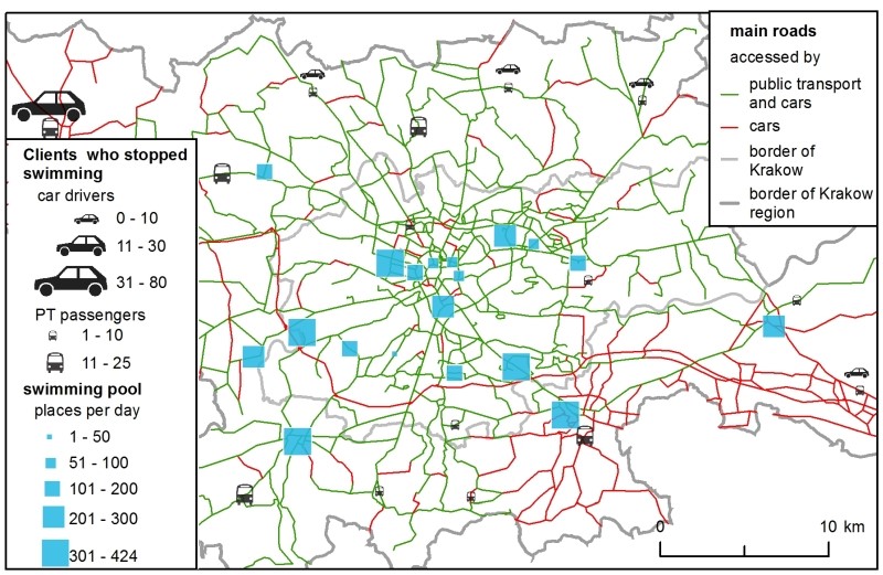
Supply is represented as the number of available places at the existing swimming pools for individual clients (Figure 1). These data were obtained from the club’s Internet sites which presented the swimming pool timetables. In the SIM, the available places were aggregated across one day, while in the H-ABM the number of places was estimated on an hourly basis as follows: after a convention used in some facilities in Krakow to ensure comfortable swimming conditions, it was assumed that one lane in a pool equalled 8 places. The total number of places was then derived from the swimming pool schedules for a single Wednesday, June 15, 2016. The choice of one day was to simplify the models in order to compare them. Wednesday was an approximation of every other weekday (the author’s survey was conducted on weekdays). The number of available swim lanes changed dynamically during a day, due to schools, aqua-aerobic clubs, etc., reserving certain lanes.
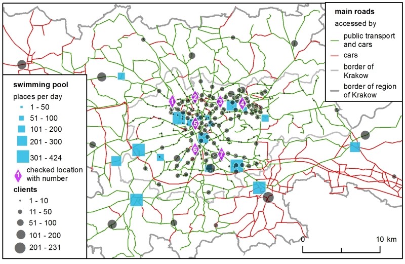
The total demand – i.e., the number of all clients in the region – was not estimated. Instead, to make calculations more straightforward, it was assumed that it was equal to the number of available places at 20 swimming pools (all the existing ones plus one new location), which gave 4,369 clients. Their spatial distribution and modal split were crucial for both models and they were estimated carefully based on numerous data sources, such as demographic data about population, a regional survey of transport preferences and a national survey on participation in sport. Figure 1 shows the spatial distribution of demand. Eventually, there were 3,693 car drivers and 676 public transport passengers (further referred to as PT passengers).
Road network distances in kilometres between clients' homes and swimming pools were calculated and then represented as distance matrices. This procedure was applied separately for drivers and PT passengers because the latter group could not use roads without public transportation.
The spatial behaviour of clients depended on the spatial accessibility of the clubs. The key reason for a client's choice of a facility – as stated by 74% of the respondents in the survey – was the amount of time needed to arrive at the swimming pool. This was reflected in the models with the application of distance decay functions. Spinney & Millward (2013) suggested the solution of a mathematical representation of travel impedance and which was implemented in the presented models. The functions were calculated separately for the drivers and PT passengers as based on the survey (more details can be found in the ODD). The latter group tended to travel on shorter distances because trams and buses are usually slower than cars.
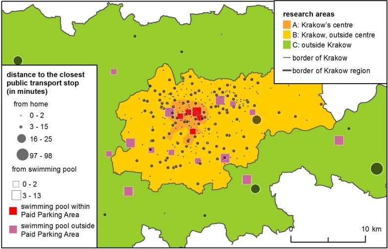
Distance decay functions did not solve the problem of the direction of movement – e.g., swimming pools in the city centre were less attractive due to traffic jams and the scarcity of parking places. In the models, this was solved by applying accessibility parameters. For drivers, all clubs located within the Paid Parking Area were less accessible and thus less attractive; – this was an approximation for congestion in the city centre. For public transport passengers, clubs located further from PT stops proved less attractive (Figure 2).
There were differences between the input data for the H-ABM and SIM. The agent-based model was temporally dynamic and each agent had a daily schedule that had to be kept. Each agent was assigned two hours of physical activity (drawn from a distribution based on the author's survey), and the swimming pools were assigned schedules with the number of places available at each hour. Furthermore, the Paid Parking Area was active only between 10 a.m. and 8 p.m. In the SIM, the total daily number of places shaped facility attractiveness and the Paid Parking Area was “always” active.
Spatial Interaction Model
In the SIM, clients were distributed across clubs based on the attractiveness and distance from their homes. The SIM consists of the same entities as the H-ABM: clients, clubs and transportation network (see Figures 1 and 2). The SIM presented here is described by the following equations (Birkin et al. 2004, p. 38):
| $$S_{ij} = A_i O_i W_j f(c_{ij})$$ | (1) |
\(O_i\) - demand for swimming pool \(j\) in origin zone \(i\);
\(W_j\) - attractiveness of facility \(j\);
\(f(c_{ij})\) - distance decay function value, where \(c_{ij}\) is a distance in kilometres between home \(i\) and club \(j\);
\(A_i\) - a balancing factor which takes account of the competition and ensures that all demand is allocated to all clubs in the region.
The attractiveness of a facility \(j\) was expressed as:
| $$W_j = L_j \text{access}_m$$ | (2) |
\(\text{access}_m\) - an accessibility parameter, dependent on client's mode of transport \(m\) (called \(\text{accessCar}\) for car drivers and \(\text{accessPT}\) for PT passengers later on). This was a value between 0 and 1.
Demand for swimming pool \(j\) incorporated the idea of elastic demand; the author used the equation proposed by Birkin et al. (2004, p. 46). This uses Hansen’s accessibility index to decrease or increase the initial demand, as written in the equation below:
| $$O_i = P_i (w_{im} w_{Ib})$$ | (3) |
\(w_i\) - a measure of access to swimming pools for clients of zone \(i\), as the Hansen's accessibility:
| $$W_i = \sum_{ij} W_j f(c_{ij})$$ | (4) |
\(b\) - a parameter dependent on clients' mode of transport m (called \({bCar}\) for car drivers and \({bPT}\) for PT passengers later on)
Hybrid Agent-Based Model
The hybrid agent-based model was built using Repast Simphony and written in Java. A short film presentation of the model can be accessed online (Kowalski 2017a; Kowalski 2017b). This was based on the RepastCity software (Malleson 2016). The complete details of the model can be found in the ODD protocol (see the Appendix).
There were two kinds of agents: 4,369 clients and 19 swimming pools. All clients wanted to swim once a day. Each client chose two preferred hours of entry to a swimming pool[1] and built a ranking of all facilities each preferred hour of the day. For example, if there were 20 swimming pools in the simulation, there would be a maximum of 40 possible choices (‘club \(x\) preferred hour’). Some swimming pools would be closed at certain hours for individual clients so the clients would disregard these. The attractiveness, \(Z\), of each club, \(j\), could then be estimated relative to the agent’s home location, \(i\), according to the following equation:
| $$Z_{ij} = f(c_{ij}) - x$$ | (5) |
At the beginning of the simulation, the \(Z\) rates of a client’s ranking for each possible choice were calculated. First, an agent chose the favourite ‘club \(x\) preferred hour’ by probability according to its Z rate – the higher the rate, the more probable it was that the agent chose it. Next, each client-agent went to their favourite swimming pool at the preferred hour. The following two situations could emerge:
- If there was a sufficient number of places available at a swimming pool for all clients, then everyone entered and all client-agents increased the Z rate of the ‘club \(x\) preferred hour’ by a value of the parameter called experience (experienceCar for car drivers or experiencePT for PT passengers).
- If there were not enough places, the swimming pool would reject some clients randomly, who subsequently decreased their rating for that ‘club \(x\) preferred hour’ choice and made a new choice on the next day. The agents who managed to enter their chosen location increased the attractiveness of their ‘club \(x\) preferred hour’ choice.
This process was repeated for seven days and the simulation ended on the last day. Unfortunately, the number seven was not supported by any research but was conceived to emphasize the potential of the agent-based models in the field of location planning. Seven days allowed the clients to make six changes in their choice based on their experience. It also made the H-ABM more dynamic because depending on the spatial interrelation between demand and supply, the client flow caused different output (further information about this design decision can be found in the discussion chapter).
Modelling Procedure in the H-ABM and SIM
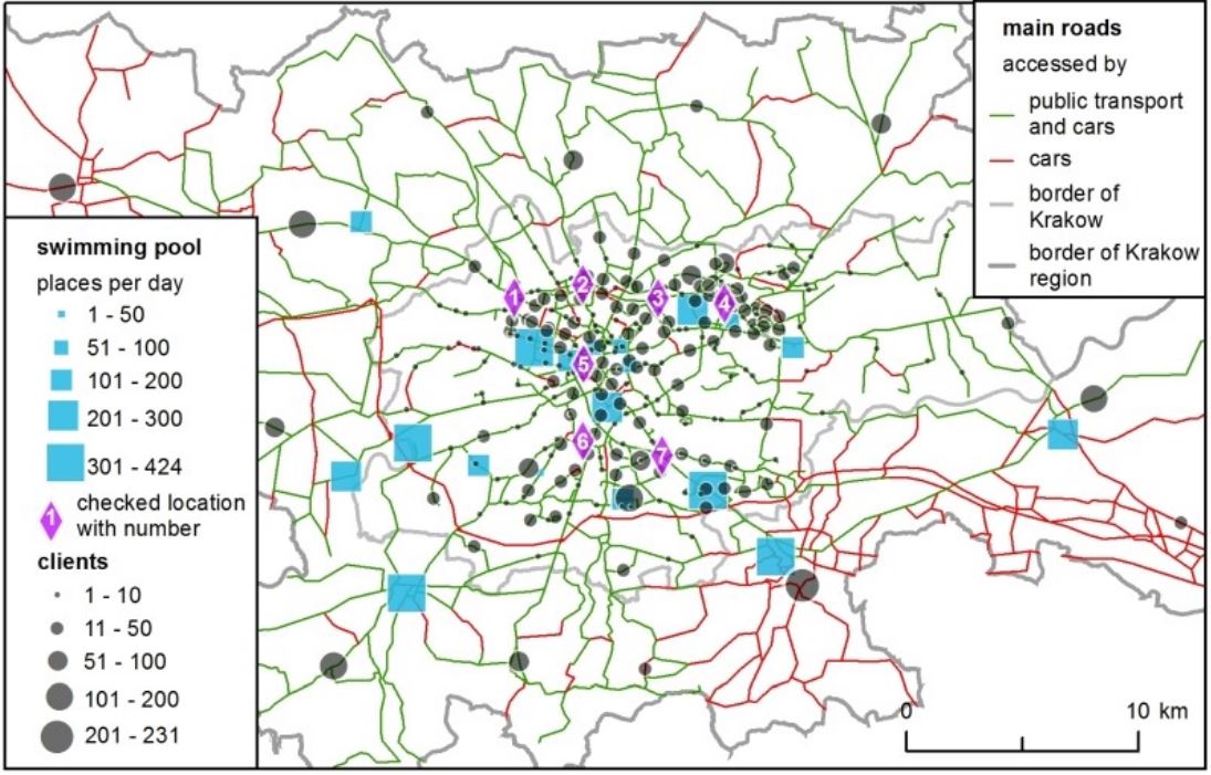
The modelling procedure presented in this article has the following structure: Initially, the models were calibrated using the existing facilities. Next, the optimal set of parameters was selected and each of the 7 checked, potential new locations for a swimming pool (see Figure 1 for the checked locations) was assessed to choose the most favourable one. The locations were chosen arbitrary, for the sake of method comparison, in well accessible places in Krakow. More locations were not considered because they would not add anything new to the discussion or the principal conclusions.
Calibration
The process of calibrating the models was designed to be simple in order to allow for an easy comparison of the modelling approaches. Detailed information about the process can be found in the Appendix.
The model fit as compared to real data (derived from the author's survey) was evaluated with three indices. An output of each simulation consisted of two matrices of home–club flows for drivers and PT passengers (similar matrices were devised from the survey). Based on this, the following fit indices were calculated:
- Spearman's rho for home-club distance-gradients of simulated and real car drivers;
- Spearman's rho for home-club distance-gradients of simulated and real public transport passengers;
- Chi-Square between the simulated and real number of clients in clubs summed up in 3 areas: A: Krakow's centre, B: Krakow, outside centre and C: outside of Krakow (see Figure 2), separately for car drivers and passengers.
The first and second indices described how far client-agents could go and the third one indicated the direction of movement. In each version of the model, four parameters influenced the output (the accessibility parameter and experience parameter - different depending on the mode of transport). The author checked model fit for 81 combinations of 4 parameter sets for the SIM and H-ABM. In each model, the best set of 4 parameters was chosen for further analysis.
Results
Sub-models only with existing facilities
In the first sub-model with existing swimming pools, the H-ABM results were more diverse than those of the SIM (Figure 3). In the SIM, rentability highly depended on the centrality of location – the facilities in the city centre were the most accessible for clients (even despite the presence of the Paid Parking Area), while those located outside Krakow were the least popular. In the H-ABM proximity played the same role, but the clubs' rentability depended on two more mechanisms: 1) clients were rejected from more popular facilities if there were no places for them at their chosen hour of entry, so 2) it was important that demand and supply matched not only spatially, but also temporally. Therefore, in the H-ABM the sites that were close to the city centre, but not directly inside it, were favoured more in the H-ABM scenario than in the SIM, as agents were forced to choose alternative facilities.
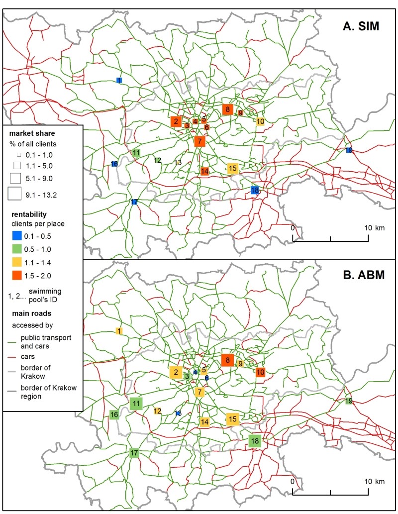
Market share followed a facility’s capacity – i.e., the total number of places it offered. This is why the most commonly chosen clubs were similar in both models, but in the SIM the difference between the clubs with the minimum and maximum market share was more prominent. In the H-ABM, the market shares were more similar between the swimming pools because of the clients’ club changing mechanism, during the simulation clients decreased the rate of any overcrowded clubs, so they ended up in less crowded alternatives.
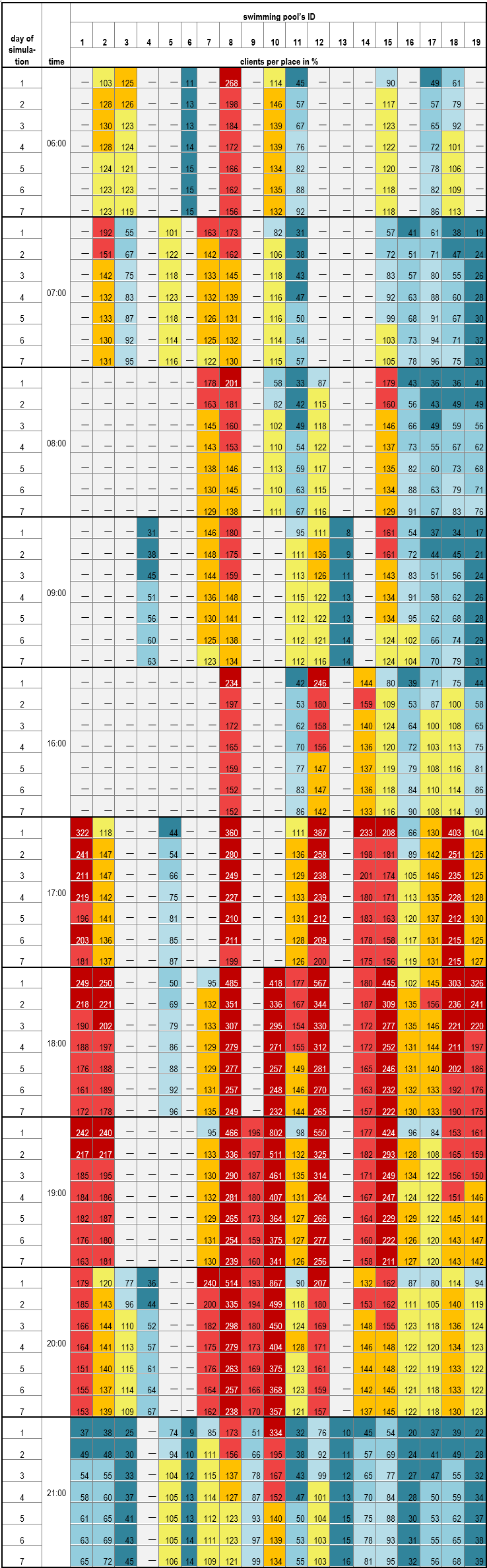
Moreover, the H-ABM was capable of generating data that showed how crowds changed in clubs by hour and day of the simulation (Table 4). This model “cooled down” – in the next days of the simulation – the client-agents were “flowing” from the most popular ‘club \(x\) hour’ opportunities to less popular ones. Since every agent chose an individual set of two preferred hours, within their ranking list, they were ”moving” not only in space but in time as well. This mechanism affected the market shares of the facilities, e.g., the most popular swimming pool no. 8 on the first day attracted 17.6% of the clients, whereas on the last, seventh day – only 10.3 %.
Furthermore, the H-ABM could also generate a map showing the clients who resigned from simulation – it resulted in the ranking in which all the possible choices were below the minimum rate (Figure 4). This map shows the unsatisfied clients – i.e., the ones who lived too far away from the closest swimming pool or those who, due to over-crowding, could not enter their chosen club. The map can be used to design a regional policy that offers better services to unsatisfied clients – whether by building a facility near their location or by improving their transport options.
Sub-Models with New Facilities
The next step was to verify which one out of the 7 locations for a new swimming pool was the ‘best’ (i.e., the one that would attract the highest number of clients). In both models, location no. 3 was the most prominent (Table 1 ). However, in the ABM there were minor differences between locations no. 2, 3 and 4, so they should be considered equally favourable. The SIM predicted a much higher market share in all the locations – on average, 47% higher.
| ABM | SIM | ||||
| checked location no. | market share in % of all clients | standard deviation of market share | rentability – clients per place | market share in % of all clients | rentability – clients per place |
| 1 | 14.13 | 0.22 | 1.13 | 18.14 | 1.37 |
| 2 | 14.45 | 0.23 | 1.13 | 21.09 | 1.62 |
| 3 | 14.76 | 0.27 | 1.16 | 23.16 | 1.80 |
| 4 | 14.61 | 0.25 | 1.14 | 22.19 | 1.72 |
| 5 | 12.40 | 0.26 | 0.97 | 18.83 | 1.42 |
| 6 | 14.00 | 0.28 | 1.09 | 20.73 | 1.58 |
| 7 | 14.01 | 0.32 | 1.10 | 20.54 | 1.60 |
Discussion – Model Comparison
Input data
The main difference between SIM and H-ABM in terms of the input data was that the latter model considered time. The agents were given two preferred hours of swimming, depending on their place of residence and the availability of lanes in clubs in the vicinity, so they had different possible choices of ‘club \(x\) preferred hour'. Globally it influenced the results and market shares because two conditions had to be fulfilled: the club offers lanes at a chosen hour and the client-agents choose it. It was not the case in the SIM because in this case, the population of clients "saw" only the total number of places as an attractiveness measure – the model distributed the clients among all facilities proportionally. In the H-ABM, the client-agents were just aware that there were certain places available, but did not know how many – they had to check it themselves. If they went there, they noted a negative or positive experience, depending on whether they did manage to swim or not.
In the H-ABM, the time of physical activity at the facility was significant for car drivers (84% of total population) because the Paid Parking Area was operable only between 10 a.m. and 8 p.m. While in the SIM, if a club was located inside the Area, it always had its rate decreased. Thus, in the SIM, the Area had a stronger effect.
Calibration
These models, by their very nature, have an entirely different philosophy of calibration and meaning for the model. Although the calibration process was reduced in both cases to checking 81 combinations of 4 parameters, the parameters had a different influence on the models. The main purpose of calibration was to create simulated results as close as possible to a real distance decay gradient of car drivers and passengers, and to a real spatial distribution of the clients in the 3 research areas (see Figure 2).
In the SIM, the interpretation of the elastic demand equations was problematic in the model with a new facility. The calculations in the SIM were made on relative numbers, and the whole demand was distributed proportionally across all the facilities. The elastic demand equations (no. 5 and 6) increased initial demand (as in the H-ABM) in places with a higher accessibility index of swimming pools. In other words, in areas with more facilities close by, a higher supply produced a higher demand, which is reasonable in the author's view, as is the case in the leisure industry (Birkin et al. 2010). Simultaneously, at places with lower index values, demand relatively decreased. The model was calibrated without a new swimming pool, so if a new one is added, the demand around it increases. On the one hand, it is reasonable, because more people are willing to swim. On the other it is not, because at the same time demand will irrationally decrease in the other areas, for people who live too far from the new object, it does not matter if it is built or not.
Demand and supply in the H-ABM were absolute values, so they had to be calculated carefully and precisely, because their inter-relation influenced the model output profoundly. For example, if there were much more places in the swimming pools than there were clients, the elastic demand parameters in the H-ABM did not matter, because all clients were happy with their closest facility. In the opposite situation, if all swimming pools had much more clients than places, they would produce more “unhappy” agents who ended their simulation prematurely.
The H-ABM coped with the problem of elastic demand quite well by means of experience parameters. For example, if some clients lived in a place without swimming pools around their home, they might give up physical activity at the end of the simulation, because many swimming pools would be too far for them and the remaining facilities might be full, so their experience would still be negative. However, if the new swimming pool was built close enough, the agents that "die" in the simulation without a new facility, would stay "alive" in the sub-model with a new facility. The effect would be only local, which is much more reasonable, than in the SIM.
The set of two parameters that controlled accessibility for car drivers and PT passengers was quite similar in both models –it could reduce the attractiveness of a club. The difference was that in the H-ABM the parameters reduced a club's rate calculated based only on distance decay function, whereas in the SIM it was also affected by available places versus the other clubs. This shows the parametrization difference between the two models. In the SIM, it is aggregated – the available places defined the significance of a swimming pool in the whole region. In the H-ABM however, the ‘available places’ were relevant only to those agents who tried to enter the swimming pool.
Models and Reality
The H-ABM was closer to reality than the SIM. It could reflect the complexity of an urban region efficiently and so is more promising for future research. This was mainly because of the following two features:
- Incorporating time-space dynamics of demand and supply of places at swimming pools and transport between them.
- Clients’ experience mechanism.
The first feature, concerning the time-space relation, enabled the H-ABM to imitate reality more closely. A client who wants to swim at 6 o'clock in the morning takes into account only those swimming pools which offer swim lanes at that hour and are located close enough to get there in time. This is the way we should think about spatial accessibility within cities.
From the perspective of club owners, the real problem lies in scheduling the available of lanes in a pool – since clubs want to meet demand optimally. According to the author's survey in Krakow's facilities, only 5% of clients came at 6:00 a.m. – which means that just a few facilities were enough to respond to this demand. Another time-space aspect was the time of the Paid Parking Area’s activity and its relation to clients’ entry to facilities located within it. This mechanism can be easily seen in Figure 3 where rentability of facilities in the city centre is more diverse in the H-ABM. Interestingly, the two preferred hours of each client and their own distance decay function generated a very diverse population of client agents. All clients had very individual "space" of ‘club \(x\) preferred hour' opportunities – it produced a quite heterogeneous population, which is recognized as a significant advantage of the H-ABM (Bonabeau 2002).
The second important H-ABM feature was the mechanism of clients' experience, which worked when clients came to the swimming pool. If there were no places for all, some of them returned home and decreased their rating of the facility. On the other hand, those who managed to swim increased the rating. There is a similar process in the real world.
According to the author's survey, the highest demand for swimming in Krakow is between 4 p.m. and 8 p.m. At this time, clubs are full and some clients cannot enter; they have to go back home and lose a few hours (there is no Internet reservation system). Overcrowded swimming pools also meant lower service quality for its clients. Many of the surveyed clients complained about too crowded lanes in the swimming pools – it was the most important issue for them because it made their sports practice uncomfortable – in a pool they had to give way to faster swimmers and take care not to hit other users accidentally. The different mechanism was a rating increase by clients who managed to swim. It reflected the situation when they got used to the circumstances and their loyalty grew. In the scale of the whole region, the clients' experience mechanism moved demand away from more popular clubs to more distant ones and it also underlined the importance of the supply-demand relation in space-time. It was closely connected with the first feature of the H-ABM. It cannot be easily replicated in the SIM, which makes it the most substantial advantage of the agent-based approach.
In the SIM, the relation between demand and supply was abstract, – e.g., if demand was set 100 times higher than supply, it would distribute it proportionally among the facilities. Theoretically, one could write an equation that made the model behave similarly to the H-ABM's experience mechanism and cut off demand higher than supply. In the author's opinion, it should be followed by incorporating space-time in the model, which is increasingly problematic with growing time complexity of the model, e.g., if the model is to use time distances that take into account the average car traffic. On the other hand, up to a certain point demand and supply were abstract also in the H-ABM. Supply was calculated just for Wednesday, not the whole week, month or year and demand was estimated based on multiple data sources. Hence, an error could occur. Demand was a delicate question in the H-ABM because it could result in clients wrongly "moved" to less popular facilities.
Practicality of the models
The SIM was a far more practical model as it was faster, easier to understand and control in terms of results. The SIM has developed since the 60's, and in recent years it is also used for business analysis to solve ‘what-if’ scenarios considering, e.g., the impact of store opening (Stillwell & Clarke 2004).
In the SIM model development and generating, results were much faster. Here, most of the actions were done in Microsoft Excel, in a number of inter-related spreadsheets. Changes could be easily implemented and it was reasonably easy to understand how the model worked as it was a matter of understanding the underlying, driving equations. In the alternative H-ABM, the issue was much more complex. One had to program and test every aspect carefully – e.g., agent behaviour, data inputs and outputs. Finally, in this example, the SIM approach proved eight times faster. Thus, modelling large and complicated systems remains a limitation of the H-ABM, because of its huge computational requirements (Parry & Bithnell 2012).
In the H-ABM, the components of the model are more interconnected, which is more realistic but less practical. In the H-ABM, a minor change of a parameter that made more car drivers appear at swimming pools in the city centre reducing the number of PT passengers there, as clients were "competing" for places and not everyone managed to enter the club. Thus, the "winners" were drawn randomly, so in fact more populous regions usually won these places. In the SIM, it was separated, a manipulation concerning similar parameters of the car drivers did not have such a major influence on PT passengers because they were not rejected by swimming pool administrators and did not ‘change their mind’. This was a benefit of the SIM, which allowed for adjusting the model quickly to real data.
Despite the many practical disadvantages of H-ABM, there are two significant advantages over the SIM: 1) its ability to reflect and visualize the aspects of complicated reality that can be important for research (see Figure 4 and Figure 5), and 2) ease of adding more complexity dimensions to the model.
Figure 4 illustrates the first advantage – crowding in clubs is a bottom-up process that was quickly visualized in the H-ABM. This information gives researchers a better understanding of the model and the real processes and enables them to present these simulated results to stakeholders that want to build a new swimming pool. In addition, it gives a new quality to the location analysis. The H-ABM is deeply visual, and it can be extremely helpful in the communication and understanding of the model (Crooks & Heppenstall 2012). The H-ABM can be analysed as a film, which presents dynamic changes in the model (see Kowalski 2017a). It is a practical advantage because the complete understanding of the model let a researcher interpret the results correctly. In the SIM one can only analyse outcomes through the input data and equations that drive the model.
The second advantage is also vital, because space-time variables in the H-ABM were significant in the presented example. Performing a similar design in the SIM would greatly complicate the model because it would require generating a vast number of spreadsheets for each new time dimension that the modeller would be required to grasp. In future, space-time could be extended to time distances, taken from sites like Google Maps, which provide information of the average traffic. The H-ABM can deal with it efficiently – clients can simply check the time distance at the specific time and place during the simulation; in the SIM aggregating space-time variables requires profound experience. Apart from the time aspect, the author's survey in Krakow has shown many other aspects that can be implemented in future versions of the H-ABM:
- Population of clients can be more diverse, certain agents can hold benefit cards that grant access to certain swimming pools.
- Different distance decay functions for age, gender groups may be applied.
- A model can include work-driven trips (they accounted for almost 20% of all trips to swimming pools, according to the author's survey).
Conclusions
The hybrid ABM can benefit from the advantages of well-established modelling techniques and add up new functionalities to existing approaches. In the author's view, a pure SIM is much more practical for simpler models with a smaller number of variables required and for models that have a single purpose. The H-ABM wins in more complicated applications that need a diverse population of clients, space-time aspect or need to make use of other H-ABM advantages, like bottom-up mechanisms. Building it on the known, equation-based model facilitates the explanation of how the H-ABM works, which is a huge advantage.
At a certain complexity point, the H-ABM meets the SIM – more complicated models are easier and faster to implement with agents. In this respect, the H-ABM proved superior to the SIM in the following two aspects:
- A swimming pool’s capacity is limited –typical of many services. Crowded facilities pose a real problem in many clubs in Krakow. It may cause clients to change their preferred places because crowding was a significant inconvenience recognized in almost every facility in the region. This scheme – here called the experience mechanism – was implemented in the H-ABM; it would be hard to replicate in the SIM.
- Space-time diversity of demand, supply and traffic are also crucial in the assessment of a market share. For clients it does matter where and when there are opened facilities because it determines their opportunity of swimming. The H-ABM could reflect and control this aspect easier.
These two issues are essential also for similar services which offer a limited number of places, i.e., recreational (e.g., fitness classes), educational (language classes) and health services (e.g., dentists).
The influence of a facility's capacity should not be essential in a certain number of situations, such as:
- when supply is much higher than demand – there is no competition for places, clients are determined for some reason to use the specific facility,
- if rush hours mean only longer queues for clients, then it has a weaker effect, because clients may be willing to wait.
Similarly, space-time should not be as crucial in retail as it is in services that provide classes at a particular time of day. Shops are usually open for a long time, so it is easier for customers to come at a given preferred hour. On the other hand, heavy traffic and overcrowded public transportation can be annoying, so "time-space" problems should be relevant especially for the shops that rely on daily shoppers, because customers who buy rarely are less vulnerable to these inconveniences. Nevertheless, diverse population is often needed in retail models, since different groups of clients tend to have different spatial behavior, mobility patterns, and product preferences. So due to this reason only, the H-ABM may be worth considering. Plus, there are also strong bottom-up mechanisms in retail, like the "lock-in", when one product becomes dominant and it is difficult for customers to switch to another, as it was the case with the QWERTY keyboard (Negahban & Yilmaz 2014).
The hybrid ABM built on well-described aggregated models are easier to communicate and enable the researchers to justify multiple modelling decisions with the existing theories. Since in future an increasing amount of disaggregated data will be available for public and commercial purposes, the author believes that the hybrid ABM will gain its advantage over purely aggregated models, like the SIM.
Acknowledgements
This paper was possible thanks to Graham Clarke and Nicolas Malleson ¬– professors from the School of Geography at Leeds University. They inspired the author and were helpful at all times.Notes
- The preferred hours were derived from probability distribution based on a popularity of certain hours – according to the author's survey.
- Algorithm was similar to one presented here: http://stackoverflow.com/questions/9330394/how-to-pick-an-item-by-its-probability. Archived at: http://www.webcitation.org/73HpELCbc.
Appendix: Supplementary information
The ODD protocol
1. Purpose
The major aim of the model presented is to provide an example of how hybrid ABM can be build based on spatial interaction model. The hybrid approach lets the researcher support his/her design decisions with a well-tested aggregated approach.
Another aim, much less important from a theoretical point of view, is to answer the question: where is the best place for a new swimming pool in a region of Krakow (in Poland)? Although SIM is not conceived for finding optimal location, it will just serve as an example for testing seven what-if scenarios. In this model, the best place is the one that will attract the highest number of clients among checked locations. Thus, the model is designed to solve a real-world scenario. It simulates the movement of clients from their homes to swimming pools (called clubs or facilities later on). Clients are divided into two groups: public transport (PT) passengers and car drivers. The main result is client distribution among all swimming pools in the region, and the optimal location is chosen. In the first step, a model is calibrated without new facilities. Next, each one of seven new locations is checked and the best one is chosen for the investment.
2. Entities, state variables, and scales
Animated presentation of the model can be accessed online (Kowalski 2017a). It is based on Nick Malleson’s RepastCity ABM (Malleson 2016). The model simulates 7 days of clients’ life and is restricted to the region of Krakow – their actions take place in a certain time of a day and place. There are 10,080 ticks. Every tick represents one minute.
There are two kinds of agents:
- Clients of swimming pools – divided into two groups: car drivers and PT passengers. Every day the agents try to get into their chosen facility at a chosen time. Every client has two preferred hours of entry to the swimming pool and, based on them, the client evaluates every choice ‘club \(x\) preferred hour’ and sets its value in a ranking from 0.000 to 1.000 points (e.g., a choice ‘club no. 1 at 6 p.m.’ could get 0.422 points) – the evaluation of the same club might differ for two chosen hours, because of the impact of accessibility indices. Agents draw favourite club based on probability – the more points a club got in client’s ranking list, the higher chance it has to be chosen by him as favourite. At the beginning of simulation, agent’s choice is based on accessibility of facilities. Later, they change the ranking based on their experience – if they could enter the swimming pool or not. The two groups of agents (drivers and PT passengers) also have their minimum rate – below it ‘club \(x\) preferred hour’ cannot be chosen as a favourite, and if no ‘clubs \(x\) preferred hour’ in a ranking has a rate above it, a client ‘dies' – resigns from ‘active live’. Everyone lives in the region of Krakow. A lot of information is fixed and represented in matrices that are read by agents at the beginning of the simulation. Therefore, every client knows: 1) their home and every club location, 2) clubs’ schedule by hour, 3) home–club distance in kilometres, 4) initial ranking points for every ‘club \(x\) preferred hour’ choice, based on distance decay function and 5) an accessibility index – the three latter (3–5) are different for car drivers and public transport (PT) passengers.
- Swimming pools are the second type of agents. They know the pool’s own schedule and they can allow only certain clients to get into their pool at a certain hour; – the number of places available change during the day. Each swimming pool agent decides if a client can enter or not, at the same time it shapes clients’ opinion about the place. They are in the same place during simulation – they cannot close and relocate to another location. Places available at certain hours do not change during following days.
The scale of a region, distribution of clients’ home, clubs and transportation network is presented below in Figure 6. All client-agents lived in homes, which were located at transportation network – more precisely it was, in fact, a population-weighted centroid of the residential area, moved on a network. Clients could move along it, but public transport passengers could only travel along bus or tram lines. Since all distances were calculated in advance and represented as matrices, agent movement along roads did not affect results and was important only for visualization and for the future development of the model (omitting this part of the code was to speed the model up).
The region of Krakow covers a total area of 1,289 km². There were 19 swimming pools with 3,840 available places and one new, checked location with 528 places. According to Central Statistical Office, there were more than 1 million inhabitants in 2012 (about 750 thousand in the city of Krakow itself). The model focused on a group of people above 20 years old, which was around 850 thousand. It was assumed that demand is equal to the supply of places – it resulted in the author’s assessment of 3,171 agent-clients, who lived in Krakow and 1,198 agent-clients outside the city centre.
3. Process overview and scheduling
The simulation was based on Nick Malleson’s RepastCity software (Malleson 2016). A short film presentation of the model can be accessed online (Kowalski 2017a).
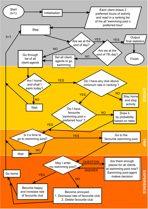
Figure 7 illustrates key processes in the simulation. In the beginning, each client chooses two different hours, when they want to start swimming (called ‘preferred hours’ later on; e.g., 4 p.m. and 6 p.m.) and they check if there is any free lane in a pool at that time. The hours are drawn according to probability based on a popularity of certain hours – according to author's survey results at swimming pools in Krakow (Table 2).
| time of entry | 6:00 | 7:00 | 8:00 | 9:00 | 16:00 | 17:00 | 18:00 | 19:00 | 20:00 | 21:00 |
| popularity in % | 5.76 | 4.68 | 4.32 | 3.42 | 3.6 | 7.74 | 14.22 | 14.04 | 17.28 | 5.94 |
Next, a client makes a ranking list of all possible ‘club \(x\) preferred hour’ choices and evaluates the choice in the following steps:
- They assesses the distance between home and the facility, according to distance decay function – the further a club is, the fewer points it gets.
- Clubs, which do not have free lanes in a pool at certain hour could not be chosen by him and get 0.000 points in the ranking.
- If the client is a car driver, they decrease the final assessment for all ‘club \(x\) preferred hour’ that are situated in a Paid Parking Zone and have an hour of entry between 10 a.m. and 8 p.m. (then the Zone was active). If they are a PT passenger, they decrease the assessment of each club based on total distance to stops (home-stop, stop-swimming pool). If a rate of a ‘club \(x\) preferred hour’ falls below minimum rate, it is changed to 0 (similarly it is changed to 1 if it exceeds 1). All ‘club \(x\) preferred hour' options are unavailable for an agent, if there are no places in the club, due to the club's schedule.
Each day, the following actions are performed:
- Choice: Clients, who do not have a favourite club (they want to go to), draw from a ranking list along with an hour of entry and remember it as a favourite club. Probability of choosing a certain club is greater for clubs with a higher ranking[2]. If in a client's ranking, there is no club with a rating higher than the minimum rate (e.g., for car drivers it was 0.0353), the client does not have a favourite club and do not take part in the simulation anymore.
- Trip: Clients travel to their favourite clubs from homes and go there exactly at a chosen hour.
- Experience: Each hour, the clubs decide who can enter and swim in a pool. If there are enough places, everyone enters. If not, the club randomly chooses clients who can enter and rejects the rest (the random number generator of java.util.Random.Random() was used for that purpose). Lucky clients increase the rating of this club and keep it as a favourite, the others decrease the rating and next day make their choice again.
Eventually, after 10,080 steps, (seven days) the program notes down which agents chooses which club and generates all output, e.g., matrix of flows between residential areas and swimming pools.
4. Design concepts
Basic principles. The ABM presented was designed to solve a real-world problem of new facility location, by simulating clients flows in the region from home to swimming pools in the first step and checking seven what-if scenarios for new swimming pools’ locations, in the second step. The model was conceived as an extension of spatial interaction models (used for the same purpose) by the idea of time-space, inspired by Hagerstrand’s geography of time, and supported by author’s survey in Krakow’s swimming pools.
Observation. The main result of the model was assigning clients to their favourite clubs and generating a matrix of flows between residential areas and sports facilities that would later on, help to decide which new locations was the best – i.e., attracted the highest number of clients. The model was also capable of showing how the crowd at swimming pools changed along simulation and map clients, who stopped swimming – i.e., who did not have any swimming pool above a minimum value in their ranking.
Emergence: During seven days of simulation, popular clubs lost their clients because there were more clients than places available at a certain hour, so the next day unhappy clients decreased their choice rate in the ranking list and they may go to another club. At the same time, less popular clubs gained new clients because unhappy clients from popular clubs could choose them. The result of simulation depended on a spatial relationship between demand and supply at a certain time during a day.
Learning: Client-agents had complete knowledge of the accessibility of all swimming pools (lanes availability, home-club distance and location of the club in Paid Parking Zone or walking distance to public transport stops). It was justified because in reality, all this information can be checked on Internet – swimming pools present their schedules and thanks to sites such as Google Maps, distances can be easily calculated. The information was used for initial ‘club \(x\) preferred hour’ rating. Later on, clients learned – they decreased rating if they did not enter a swimming pool, which showed their annoyance or increased it, if they swam – which reflected stronger loyalty and their happiness.
Stochasticity. This was present in three situations:
- Clients drew their two preferred hours of entry, according to probability calculated based on a popularity of certain hours (Table 2). It generated crowding in clubs during rush hours at the beginning of the simulation, which was later on, split into less popular clubs or hours. Apart from this, this action determined spatial distribution demand for certain hours – it was more likely that there would be more “early birds” (clients choosing 6 or 7 a.m.) in more populated areas.
- A client surrounded by clubs with a similar rating in their ranking, had quite equal chance of being chosen as favourite. It resulted in a situation where a client may be “locked” in their path, and they would stick to their choice to the end of the simulation. However, the result of simulation was a mean of 30 model runs, so the effect of lock-in was not very strong. The situation was the opposite if there was only one club in client’s vicinity – even if the client did not enter, next day they would choose it anyway because there would be no other strong alternative choice.
- Clients, who could not get in a pool (because of the limit) were rejected randomly. It seems to be the most random mechanism in the model. However, at the level of results, it was not random – more densely populated neighbourhoods were more likely to be represented in the club in simulation output, because of their size.
Heterogeneity. Interestingly, the model generated a very diverse population of client-agents, each one with very individual “space” of opportunities, within which the client chose a favourite club. It was an effect of client’s home location merged with his own distance decay function (different for drivers and PT passengers) and with two preferred hours of entry.
5. Initialization
There were eight sub-models. In the first one, there were only 19 swimming pools that altogether had 546 lanes, equal to 4,368 places. In the next seven sub-models, one new location was checked, so there were in fact 528 more places. Demand – a number of clients and their home location – stayed at the same level during all simulations and was equal to the number of places in all existing swimming pools and one new location. Clients drew two preferred hours and a favourite club, as it described in ‘Process overview and scheduling’. Demand was roughly equal to supply – there were 3,693 car drivers and 676 PT passengers (Figure 6). Minimum rate for drivers was equal to 0.03530 and for PT passengers to 0.01208. These two numbers were equal to the value of distance decay functions for 22 km for car drivers and 16 km for PT passengers – for model output it meant that minimum rate determined agent’s maximum distance. In the first step of each simulation, all client–agents built their individual ranking of swimming pools and took all necessary information from pre-calculated matrices.
There were types of 4 matrices: home–club distances, initial club rate (values of distance decay function for home–club distances), accessibility indices and facilities’ schedules. First three were different for car drivers and PT passengers. The last one was used by each client, but also by every swimming pool-agent. All initial values stayed the same during all simulation (demand, supply, distances, distance decay functions, and other parameters). The only initial values set stochastically were two preferred hours of sports activity.
The most important data source was author’ survey in Krakow – its results were used as input data, as well as a support for many design decisions. The survey was conducted between March and November 2014. 517 questionnaires were gathered at 14 swimming pools (out of 20) – 437 from car drivers and 79 from PT passengers who lived in Krakow's region. It was convenience sampling; – in the first step swimming pools were chosen randomly, in the second survey was conducted for a whole day in a facility with all its clients, who agreed to take part in it. In all 14 clubs surveyed, population was very similar to a swimming population that was surveyed in a national survey on physical activity (GUS 2013), which proves its quality. An English version of the questionnaire is attached at the end of this document available online (Kowalski 2017b).
Supply was represented as a number of available places in swimming pools. Schedules were presented on a website of every facility. The author used schedules for Wednesday, 15th June 2016 to calculate a number of available lanes in each swimming pool at certain hours. He calculated the number of places, with an assumption that there can be only eight swimmers in each lane. Limit of eight persons was a reasonable number used by some swimming pools in Krakow to calculate how many clients they can receive.
Author assessed spatial distribution of demand in following steps:
- Number of people in each age group (20¬–29, 30–39, 40–49, 50–59 and more then 60 years old), living in all 377 residential areas in the Krakow region, was multiplied by percentage of active population in each age group, taken from national survey on participation in physical activity (GUS 2013). The number of people in each area was based on spatial demographic data for 2012 official from Central Statistical Office (areas outside Krakow) and commercial data from GFK Polonia (areas inside Krakow). A decline in sports participation with age (older people are less likely to swim, then younger ones) was recognized by other authors, like Breuer et al. (2010) and Farrell & Shields (2002), as well as in the cited national survey ( GUS 2013).
- Next, the population of clients was divided into car drivers and public transport passengers, similarly according to the same age groups, based on results of Comprehensive Travel Survey in Krakow (Szarata 2014).
- Total number of car drivers in each residential area was multiplied by 0.82 and passengers by 0.18, to keep global proportion of mode of transport used at the same level as in author’s survey, conducted in 14 swimming pools in Krakow’s region (proportion of population travelling by public transport from the previous step was not coherent with the author's survey in clubs).
- Eventually, total demand was reduced to the level of all available places with one new facility (otherwise there would be a great overestimation of demand – (34 clients per available place at swimming pool).
Distances between homes (population-weighted centroids of residential areas) and swimming pools were calculated in kilometres along roads in ArcGIS, using Network Analyst, separately for car drivers and public transport passengers (these were the only modes of transport considered). Distances to bus or tram stops were represented in minutes and were calculated using krakow.jakdojade.pl website, which is designed to help passengers find their best route. One residential area was not accessible by public transport because its centroid laid about 5 km away from the network.
Eventually, the attractiveness of a swimming pool for passengers decreased, based on a sum of time distances to public transport stops (home-stop, stop-club) and for car drivers, if it was situated in Paid Parking Zone – there were six swimming pools in total (Figure 8). Model parameters influenced the strength of decreased attractiveness in agent’s ranking.

Distance decay functions were calculated based on results of author's survey with swimming pools' clients. The author calculated respondents home–club distance in km and similarly to Skov-Petersen (2001). He used a negative exponential function and calculated beta parameters separately for car drivers (0.152) and passengers (0.276). Curve estimation was done in IBM SPSS Statistics 23 with curve fitting module, as recommended by Iacono et al. (2008). The goodness of fit (R-squared) of the two distance decay functions to an inversed relative accumulated number of trips was very high (0.990 for drivers and 0.958 for passengers).
6. Input data
The model did not use input data to represent time-varying processes. All information was transferred to agents and environment at the beginning of simulation (which was described at Initialisation).
Sub-models
There were eight sub-models (all built in Java in Repast Simphony and Eclipse). In the first one, there were only existing swimming pools. It was used to calculate the best parameters values, that were used later on in the next seven ones with every new, checked swimming pool. In those 7, market share was calculated, and at the end, the best location was chosen, which was the one that attracted the highest number of clients.
The most important process that influenced simulation's result was client's assessment of every swimming pool at the beginning and experience, which resulted in club ranking update. The initial ranking of each facility was calculated according to the following equation:
| $$Z_{ij} = f(c_{ij}) - x$$ | (6) |
\(x\) – a value, by which distance decay function value was decreased – controlled by parameters: trafficImpact (for car drivers) or PTStopDistanceImpact (for PT passengers; see Table 3). Calculation of x value for PT passengers was specific because it was based on time distances to stops from home and clubs (different for every home-club combination). The calculation was determined by the following equation:
| $$x = (d_{is} + d_{js}) / \textit{PTStopDistanceImpact}$$ | (7) |
Later on, the client’s ‘club \(x\) preferred hour’ possibility \(Z_{ij}\) was decreased or increased by experienceCar or experiencePT parameters, based on their experience in the club.
If \(Z_{ij}\) was greater than 1, it was changed to 1, if lesser than the minimum rate, it was changed to 0. Choices with rate lesser than minimum rate were rejected by a client and moreover, if an agent did not have any club with a rate greater than the minimum, they resigned from the simulation.
All parameters used in ABM are listed below.
| Agent influenced by parameter | Parameters | Effect on model output |
| Car driver | trafficImpact | Higher value means that there are fewer car drivers in a city centre. It is valid for every club that is situated in Paid Parking Area and clients’ time of entry is between 10 a.m. and 8 p.m. |
| Public transport passenger | PTStopDistanceImpact | A lower value means that sum walking distances to stops have a greater influence on client choice |
| Car driver | experienceCar | The strength of client's experience in a club. Higher value means that clients will be more likely to choose another club or resign faster from simulation |
| Public transport passenger | experiencePT | – if there is no club with rate higher than minimum rate |
Parameterisation
The result of each simulation consisted of two matrices of home–club flows. Based on this, three fit indices were calculated:
- Spearman's rho for home-club distance-gradients of simulated and real car drivers (correlation method in Java library: org.apache.commons.math3.stat.correlation.SpearmansCorrelation),
- Spearman's rho for home-club distance-gradients of simulated and real public transport passengers (method as above),
- Chi-Square between real and simulated number of clients in clubs summed up in 3 areas: A: Krakow's centre, B: Krakow, outside centre, and C: outside of Krakow (see Figure 8), separately car drivers and passengers (chiSquareDataSetsComparison method in Java library: org.apache.commons.math3.stat.inference.ChiSquareTest).
In each version, there were four parameters that influenced the output. The author checked different values for every parameter – there were 81 combinations. Each combination was checked three times (because of model stochastic nature) and mean values of the fit indices were used later on. Eventually, a standard score for every index was calculated, and a mean value of the three scores was a result of parametrization – a combination with the highest value was chosen for next stages of modelling.
Following combination of values for four parameters were checked:
trafficImpact: 0.1, 0.3, 0.5,PTStopDistanceImpact: 30, 50, 150,
experienceCar: 0.1, 0.3, 0.5,
experienceBus: 0.1, 0.3, 0.5.
It should be noted that if a sum of distances to PT stops was equal to 15 minutes – x parameter was equal to 0.1, 0.3 or 0.5, depending on PTStopDistanceImpact value (see Equation 7).
Statistics of a model with the best combination of parameters is presented in Table 6. Data used for the calculations in Table 6 is presented in Tables 7 and Table 8. Statistics of all 81 combinations are shown in Table 7. In the short model, the fit was very good for all combinations checked.
| Mean | Standard deviation | ||
| Spearman's rho for home-club distance-gradient | 1. Car drivers | 0.87 | 0.03 |
| 2. Public transport passengers | 0.94 | 0.02 | |
| 3. Chi-Square , number of clients in clubs summed up in 3 areas | 11.98 | 2.30 |
| Mean of transport | Data | Home-club distance in kilometres | |||||||||||
| 0-2 | 2-4 | 4-6 | 6-8 | 8-10 | 10-12 | 12-14 | 14-16 | 16-18 | 18-20 | 20-22 | sum | ||
| % | |||||||||||||
| Car | simulated | 3.0 | 11.1 | 13.0 | 12.5 | 11.5 | 10.6 | 11.3 | 9.6 | 8.8 | 5.0 | 3.7 | 100.0 |
| Empirical | 5.3 | 14.4 | 26.3 | 17.6 | 11.7 | 6.4 | 5.9 | 4.8 | 3.9 | 1.1 | 1.1 | 98.5 | |
| public transport | simulated | 10.1 | 25.5 | 24.6 | 22.7 | 10.6 | 4.4 | 2.1 | 0.0 | — | — | — | 100.0 |
| empirical | 6.3 | 20.2 | 31.6 | 17.7 | 16.5 | 1.3 | 5.1 | 1.3 | — | — | — | 100.0 | |
| Data | Mean of transport | ||||||
| Car | Public transport | ||||||
| Research areas | sum | ||||||
| A: Krakow's center | B: Krakow, outside center | C: outside Krakow | A: Krakow’s center | B: Krakow, outside center | C: outside Krakow | ||
| % | |||||||
| Simulated | 8.2 | 50.2 | 29.4 | 3.9 | 7.8 | 0.6 | 100.0 |
| Empirical | 9.5 | 43.1 | 31.9 | 6.2 | 8.7 | 0.6 | 100.0 |
| Parameter number | Mean | Standard deviation | Median | Minimum | Maximum |
| 1 | 0.83 | 0.05 | 0.83 | 0.71 | 0.90 |
| 2 | 0.90 | 0.02 | 0.90 | 0.80 | 0.94 |
| 3 | 22.87 | 8.44 | 20.67 | 11.86 | 40.73 |
Model outputs
Next, eight sub-models were checked with the combination of best parameters. Each model was checked 30 times and mean values were used later on for output presentation – according to Abdou et al. (2012) 30 model runs is a reasonable number for ABM, and low standard deviation of results for presented models proved it is true for this one.
Sub-model without new facilities
In a basic model, without new locations, in general clubs' market share and rentability depended on a spatial relationship between demand and supply, that was driven by distance decay function – closer residential areas and bigger ones usually were better represented within club's clientele group (Figure 9). Usually, swimming pools that offered more places had a higher market share. The number of clients decreased in the city centre, because of parameters that lowered the number of drivers there. This was vital for clubs because drivers consisted 84% of demand (Figure 10–11). A novelty in the presented model is that output also depended on:
- Time-space accessibility – clubs that didn’t respond to demand at the right time got lower rentability,
- Clients’ interaction in clubs – some demand was split into other clubs.
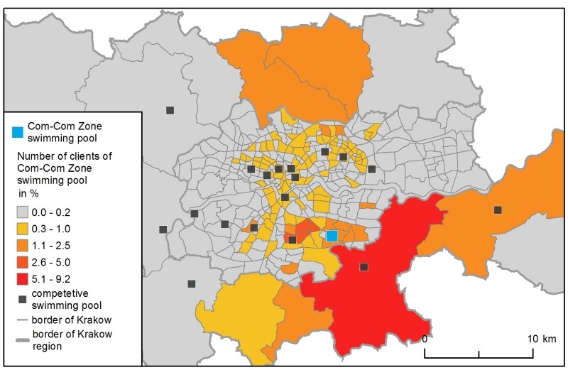
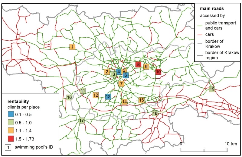
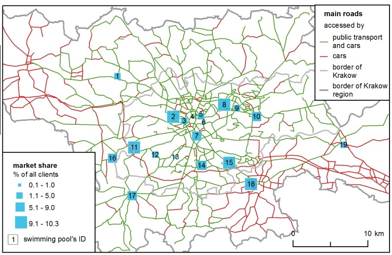
Figure 12 show how crowded were swimming pools at certain hours and how it changed during simulation. If there was no place for an agent – they could change their club (more specifically, he could change ‘club \(x\) preferred hour’ choice). The most popular facilities, like no. 8, lost their clients along simulation. A popular club could possibly gain new clients because other clubs lost them (e.g., club no. 16 at 17:00 and 18:00). Another situation was that all swimming pools with less than 100% of their capacity gained new clients or remained at the same level (the table presents the mean of 30 simulations, so there can be small deviations from that rule). E.g., the facility no. 18 in the 1st day at 6:00 had 61% of capacity and in the 7th day – more than 100%. These results correspond author’s survey in Krakow – club capacity and problems with space were the most common complaints among respondents. Moreover, Figure 12 opens new analytical possibilities as it can be used for smarter schedule planning of one or more swimming pools in the city, to optimize their schedules.

ABM simulation “cooled down” during seven days and approached an equilibrium in which each swimming pool would have 100% of its capacity (Table 7). In fact, the equilibrium was never reached, the model shows six possible changes of each clients’ choice. This mechanism showed how much facilities were susceptible to concurrence. The most vivid example here is facility no. 8 – market share decreased from 17.6 % to 10.3%, which meant that it was roughly equal to the market share of facility no. 2 and no. 15, primarily because standard deviations from 30 simulations at seventh day for those 3 were between 0.26 and 0.28%.
| Day of simulation | Swimming pool no. | Sum | ||||||||||||||||||
| 1 | 2 | 3 | 4 | 5 | 6 | 7 | 8 | 9 | 10 | 11 | 12 | 13 | 14 | 15 | 16 | 17 | 18 | 19 | ||
| % of all clients | ||||||||||||||||||||
| 1 | 4,0 | 9,8 | 1,8 | 1,9 | 0,4 | 1,2 | 0,2 | 17,6 | 3,4 | 7,6 | 6,2 | 5,9 | 0,1 | 7,0 | 10,6 | 3,4 | 5,2 | 7,3 | 6,2 | 100,0 |
| 2 | 3,8 | 10,5 | 2,1 | 2,0 | 0,5 | 1,5 | 0,2 | 13,7 | 3,8 | 6,5 | 7,6 | 4,9 | 0,1 | 7,2 | 10,3 | 4,4 | 6,3 | 8,0 | 6,7 | 100,0 |
| 3 | 3,5 | 10,3 | 2,4 | 2,0 | 0,6 | 1,6 | 0,2 | 12,2 | 4,0 | 6,4 | 8,1 | 4,8 | 0,1 | 6,9 | 10,2 | 4,8 | 6,9 | 8,4 | 6,5 | 100,0 |
| 4 | 3,5 | 10,2 | 2,5 | 2,0 | 0,6 | 1,7 | 0,3 | 11,5 | 4,1 | 6,2 | 8,5 | 4,7 | 0,1 | 6,7 | 10,1 | 5,0 | 7,2 | 8,7 | 6,4 | 100,0 |
| 5 | 3,4 | 10,2 | 2,6 | 2,1 | 0,7 | 1,7 | 0,3 | 11,0 | 4,2 | 6,0 | 8,7 | 4,5 | 0,1 | 6,6 | 10,1 | 5,2 | 7,4 | 9,0 | 6,4 | 100,0 |
| 6 | 3,4 | 10,0 | 2,6 | 2,0 | 0,7 | 1,8 | 0,3 | 10,7 | 4,3 | 5,9 | 8,9 | 4,4 | 0,1 | 6,4 | 10,0 | 5,3 | 7,5 | 9,2 | 6,3 | 100,0 |
| 7 | 3,3 | 10,1 | 2,6 | 2,1 | 0,8 | 1,8 | 0,3 | 10,3 | 4,4 | 5,8 | 9,1 | 4,4 | 0,1 | 6,4 | 9,9 | 5,5 | 7,6 | 9,4 | 6,2 | 100,0 |
The model was also capable of reducing demand if supply was too low. Each day, roughly 70 agents stopped their activity because they did not have any swimming pool in the ranking above the minimum rate. In the end, 6.9% resigned. They usually lived outside Krakow (Figure 8.). This information could also be useful for future facility planning and mapping potential problem areas – places with poor access to certain services.
Clients, who stopped swimming, did not have any swimming pool above the minimum value in their ranking.

Sub-models with new facilities
The last step was to check which out of 7 possible locations for a new swimming pool gave the highest number of clients. As a result of this analysis, there were three equally good locations, because of high standard deviations and small differences between their market shares (Table 9). Rentability of all, except no. 5, located in the city centre were very good – above 1, which means there were on average more clients than places.
| Checked location no. | Market share in % of all clients | Standard deviation of market share | Rentability – clients per place |
| 1 | 14.13 | 0.22 | 1.13 |
| 2 | 14.45 | 0.23 | 1.13 |
| 3 | 14.76 | 0.27 | 1.16 |
| 4 | 14.61 | 0.25 | 1.14 |
| 5 | 12.40 | 0.26 | 0.97 |
| 6 | 14.00 | 0.28 | 1.09 |
| 7 | 14.01 | 0.32 | 1.10 |
Discussion
There are design decisions that need to be adequately explained, because they may be controversial.
- Wednesday (15th June 2016) was chosen to gather information about lane availability and schedules of swimming pools. This day was a proxy of all weekdays. It was an arbitrary choice, made to simplify all calculations. Ideally, it should be done for all days of the week during the whole year (because of the seasonality of physical activity) – unfortunately, this solution would require more data on supply side about available lanes and demand side about clients: day preferences and frequency of sports practice. More sophisticated versions of this model will require much more time for performing simulations, and they will be unrealistic without any simplifications.
- Potential client populations and swimming pools from outside the region of Krakow were not taken into account. This is a common problem in this kind of models. In this example, it should not generate significant bias. According to the author’s survey, only 7.4% of clients came from outside of research area.
- Demand assessment was difficult. Initially, it was much bigger than supply. This was because its calculation was based on the national survey (GUS 2013), where they asked if respondent swam during last year. It was the best and the most reliable source of data, which included swimming and not-swimming population, but eventually it led to very unrealistic calculations that reflected a number of swimmers during the whole year, rather than a single day (34 clients per available place at a swimming pool). Therefore, total demand was reduced to the level of supply of places available during one day. That action did not influence the results much – it was a shortcut that improved ABM performance because anyway if demand was much higher than supply, many clients would not find their place and they would resign anyway. What mattered the most was the spatial distribution of clients, which influenced final results and optimal location choice.
- Kilometres were a good measure of distance because it considered used mode of transport (Spinney & Millward 2013). Ideally, it should be time distances that take into account traffic jams at rush hours.
- Distance decay function influenced the model’s result considerably. This was supported by the author’s survey – the fact that clients could come to a swimming pool quickly was very important for them (valid for 74% of respondents).
- Maximum distance was a result of minimum rate, below which a facility was not considered. It was inspired by research from Germany (Wicker et al. 2009), where respondents indicated maximum distance they can go to the closest sports facility. It was also a reasonable assumption because sports services are supplementary in contrast to healthcare services, so if the closest swimming pool is too far away, a client can decide on different physical activity, more accessible for them (like running in a park).
- Parametrization was done at very general level. Spearman’s coefficient and Chi-Square controlled only directions of flows and level of demand at specific areas, but they were not very powerful. Home-club distance-gradients did not have a normal distribution, so Pearson's coefficient could and R-squared statistics not be used. Moreover, distance decay function merged with maximum distance influenced Spearman's coefficient a lot. Unfortunately, these coefficients were the only possible ones. The survey that was used to calibrate the model was done in many clubs, and there were only a few questionnaires from each facility, so the only data that could be used was the one presented. Ideally, it would be to compare simulated, and real client’s home locations for few facilities and check model fit with Pearson’s coefficient, which is more powerful. On the other hand, presented distance decay functions were calculated based on the survey in many facilities, which let them generalize real distance decay better than if it would be done only based on few facilities (here results could be more biased locally).
- The model was susceptible to the demand and supply relationship. If wrongly calculated, it influenced parametrization process and final results. The demand level was an assumption, but if it was much higher, it may have been unrealistic and led to longer model runs and worst performance. If it was too low, there would be no interaction between agents in swimming pools – everyone would swim. In reality, there was an interaction, according to the author's survey, and the lack of space in a pool was the most critical issue for respondents and when rush hours pools were full, some clients did not get in.
- In 7 sub-models with new locations, the model was susceptible to the number of lanes available and hours of entry of checked facility. Smaller swimming pools would have smaller spatial influence, and therefore different location would be indicated by the model.
- Clients chose two preferred hours. This number was taken arbitrarily. In fact, there was no good data about the preference, and there should be some research to solve this problem. We do not know how many hour preferences have clients, how does it differ by age or gender or what is more important: an hour of activity or a club. Referring to international research may be misleading here – it may vary very much locally, because of traffic jams, working time and population structure. According to author's survey, 19% of respondents came irregularly or frequently came at more than two chosen hours, the rest preferred one or two hours.
- experience parameter was designed to reflect clients’ feelings about swimming pool – fidelity or rejection. There was an assumption that these two feelings had the same impact on club assessment in ranking. Indirectly this parameter let the model reflect demand elasticity (Birkin et al. 2010) – if there were new locations checked (in 7 sub-models), there was more supply and final demand was higher, because more agents end up the simulation with the favourite club. These were usually clients, who lived in the vicinity of the new facility.
- The model was stochastic in three cases: clients draw two preferred hours based on probability (taken from the survey), clubs with similar rating could be drawn as favourite by clients with similar probability, and if there were more clients than places, clubs rejected some clients randomly (it was explicitly explained and justified in Design concepts chapter). Eventually, final matrices of flows (between clients’ homes and they preferred clubs) were very similar in 30 model runs, e.g., a standard deviation of market share for seven checked locations was smaller than 0.33 % of market share (see Table 12 ).
- The last and the most important, the controversy was that simulation ended precisely after seven days. In fact, this action reflected six possible changes of a club and results showed the resilience of all locations to these changes – its dynamics are presented in table 7 and 8. Alternatively, the simulation could end after the first day, but then there would be no interaction between clients, and that would be in a contrary to survey results and author's observation. Alternatively, it could end if no agent changes his favorite club – in this case, it would be hard to choose the best location because all of them would have very similar market shares.
References
ABDOU, M., Hamill, L. & Gilbert, N. (2012). 'Designing and building an agent-based model.' In A. J. Heppenstall, A. T. Crooks, L. M. See & M. Batty (Eds.), Agent-Based Models of Geographical Systems. Berlin/Heidelberg: Springer, pp. 141–165.
ATHANASIADIS, I. N., Mentes, A. K., Mitkas, P. A., & Mylopoulos, Y. A. (2005). A hybrid agent-based model for estimating residential water demand. Simulation, 81(3), 175-187.
BIRKIN, M., Clarke, G., Clarke, M. & Culf, R. (2004). 'Using Spatial Models to Solve Difficult Retail Location Problems.' In Stillwell, J. & Clarke, G. (Eds.), Applied GIS and Spatial Analysis. Wiley Online Library, pp. 35–41.
BIRKIN, M., Clarke, G. & Clarke, M. (2010). Refining and Operationalizing Entropy-Maximizing Models for Business Applications. Geographical Analysis, 42(4), 422–445.
BONABEAU, E. (2002). Agent-based modelling: Methods and techniques for simulating human systems. Proceedings of the National Academy of Sciences of the United States of America (PNAS), 99 (3), 7280–7287.
BREUER, C., Hallmann, K., Wicker, P. & Feiler, S. (2010). Socio-economic patterns of sport demand and ageing. European Review of Aging and Physical Activity, 7(2), 61–70.
CLIQUET, G. (2006). Geomarketing: Methods and strategies in spatial marketing. Chichester: John Wiley & Sons.
CLARKE, G. P., & HAYES, S. (2006). 'GIS and retail location models.' In Cliquet, G. (Ed.), Geomarketing: Methods and Strategies in Spatial Marketing. Chichester: John Wiley & Sons, pp. 165-186.
CROOKS, A. T., & Heppenstall, A. J. (2012). 'Introduction to agent-based modelling.' In A. J. Heppenstall, A. T. Crooks, L. M. See, M. Batty (Eds.), Agent-Based Models of Geographical Systems. Berlin/Heidelgerg, Springer, pp. 85-105.
DEARDEN, J., & Wilson, A. (2012). 'The Relationship of Dynamic Entropy Maximising and Agent-Based Approaches in Urban Modelling.' In A. J. Heppenstall, A. T. Crooks, L. M. See, M. Batty (Eds.), Agent-Based Models of Geographical Systems. Berlin/Heidelgerg, Springer, pp. 271-308.
FARRELL, L. & Shields, M. A. (2002). Investigating the economic and demographic determinants of sporting participation in England. Journal of the Royal Statistical Society: Series A (Statistics in Society), 165(2), 335–348.
GIABBANELLI, P. J., Gray, S. A., & Aminpour, P. (2017). Combining fuzzy cognitive maps with agent-based modeling: Frameworks and pitfalls of a powerful hybrid modeling approach to understand human-environment interactions. Environmental Modelling & Software, 95, 320-325.
GUS (2013). Uczestnictwo Polaków w sporcie i rekreacji ruchowej w 2012 r. Warszawa: GUS.
HALLMANN, K., Wicker, P., Breuer, C. & Schӧnherr, L. (2012). Understanding the importance of sport infrastructure for participation in different sports-findings from multi-level modelling. European Sport Management Quarterly, 12(5), 525–544.
HEINEMANN, K. (2005). Sport and the welfare state in Europe. European Journal of Sport Science, 5(4), 181-188.
HEPPENSTALL, A., Evans, A. and Birkin, M. (2006). Using Hybrid Agent-Based Systems to Model Spatially-Influenced Retail Markets. Journal of Artificial Societies and Social Simulation 9(3), 2: https://www.jasss.org/9/3/2.html.
HIGGS, G., Langford, M. & Norman, P. (2015). Accessibility to sport facilities in Wales: A GIS-based analysis of socio-economic variations in provision. Geoforum, 62, 105–120.
IACONO, M., Krizek, K. & El-Geneidy, A. M. (2008). Access to destinations: how close is close enough? Estimating accurate distance decay functions for multiple modes and different purposes, (pp. 11). https://conservancy.umn.edu/bitstream/handle/11299/151329/Mn_DOT2008-11.pdf?sequence=1&isAllowed=y.
KOWALSKI, L. (2017a). Presentation of an agent-based model of swimming pools' location analysis. https://www.youtube.com/watch?v=tDTtcscyTdI.
KOWALSKI, L. (2017b). Questionnaire of swimming pools, fitness clubs and yoga schools' clients. https://www.researchgate.net/publication/315688521_swimming_pools_fitness_clubs_and_yoga_schools_clients_questionnaire.
MANLEY, E., Cheng, T., Penn, A., & Emmonds, A. (2014). A framework for simulating large-scale complex urban traffic dynamics through hybrid agent-based modelling. Computers, Environment and Urban Systems, 44, 27-36.
MALLESON, N. (2016). RepastCity. https://github.com/nickmalleson/repastcity/. Archived at: http://www.webcitation.org/73HlMVIVN. MALLESON N. (2017). RepastCity. https://github.com/nickmalleson/repastcity/. Archived at: http://www.webcitation.org/73HlMVIVN.
MURRAY, A. (2010). Advances in location modelling: GIS linkages and contributions. Journal of Geographical Systems, 12(3), 336.
NEGAHBAN, A., & Yilmaz, L. (2014). Agent-based simulation applications in marketing research: an integrated review. Journal of Simulation, 8(2), 129-142.
PARRY, H. R., & Bithell, M. (2012). 'Large scale agent-based modelling: A review and guidelines for model scaling.' In A. J. Heppenstall, A. T. Crooks, L. M. See, M. Batty (Eds.), Agent-based models of geographical systems. Berlin/Heidelberg: Springer, pp. 271-308.
PAWLOWSKI, T., Breuer, C., Wicker, P. & Poupaux, S. (2009). Travel time spending behaviour in recreational sports: An econometric approach with management implications. European Sport Management Quarterly, 9(3), 215–242.
SALZE, P., Banos, A., Oppert, J.-M., Charreire, H., Casey, R., Simon, C., Chaix, B., Badariotti, D. & Weber, C. (2011). Estimating spatial accessibility to facilities on the regional scale: an extended commuting-based interaction potential model. International Journal of Health Geographics, 10, 2.
SKOV-PETERSEN, H. (2001). Estimation of distance-decay parameters: GIS-based indicators of recreational accessibility. In ScanGIS (pp. 237–258).
SPINNEY, J. E., & Millward, H. (2013). Investigating travel thresholds for sports and recreation activities. Environment and Planning B: Planning and Design, 40(3), 474-488.
STILLWELL, J. & Clarke, G. (2004). Applied GIS and Spatial Analysis. Chichester: Wiley.
SZARATA, A. (2014). Kompleksowe badania ruchu w Krakowie w 2013 r.-wybrane wyniki. Logistyka, 6.
WICKER, P., Breuer, C. & Pawlowski, T. (2009). Promoting sport for all to age-specific target groups: The impact of sport infrastructure. European Sport Management Quarterly, 9(2), 103–118.
WU, B. M., Birkin, M. H., & Rees, P. H. (2011). A dynamic MSM with agent elements for spatial demographic forecasting. Social Science Computer Review, 29(1), 145-160.