
Introduction
Agent-based models (ABMs) are a type of computer simulation made up of agents that can interact with each other and with an environment (Gilbert 2008). They are a popular tool in many fields because they allow for a greater flexibility when creating the model compared with more common methods such as mathematical modelling. ABMs can also capture unexpected aggregate phenomenon that result from combined individual behaviours in a model, which can lead to more accurate epidemiological modelling (Bruch & Atwell 2015).
One area where ABMs are particularly useful is infectious disease epidemiology, this is because ABMs can capture the dynamics of the disease spread combined with the heterogeneous mixing and social networks of the agents (Bobashev et al. 2007). In order to be able to realistically model an outbreak and to be useful in real world scenario the model needs to be based on data and include the appropriate level of detail. If the right level of detail is used an ABM can produce accurate results. These details include not only characteristics of the disease such as infection rates but characteristics of the agents as well (Hunter et al. 2017). In an infectious disease model the demographic and socioeconomic characteristics of an agent can affect the health of the agent.
Many studies have found that demographic and socioeconomic factors can have an influence on individual health (Mackenbach et al. 2007; Doherty et al. 2014; Jessop et al. 2010; Endrich et al. 2009). Across Europe, there is a trend of higher morbidity and mortality among those with lower levels of income and or education, both factors that contribute to an individual’s socioeconomic status (Mackenbach et al. 2007). Although there are many ways in which socioeconomic factors can affect health, in relation to the spread of infectious diseases one major factor is vaccination rates. A number of studies have shown that various demographic factors can have an effect on vaccination status. Doherty et al. (2014) studied the inequality in childhood vaccination status in Ireland and found that the majority of the vaccination inequality can be explained by socioeconomic variables. They found that socioeconomic status, household structure and equalized income explained most of the inequality in vaccination status, but also that a mother with non-Irish ethnicity reduces the inequality in vaccinations while an employed mother increases this inequality. Jessop et al. (2010) studied predictors for the uptake of the first MMR vaccine and determined that a higher level of MMR vaccination was found among children with working mothers, and higher income families. Lower levels of vaccination were found among children with degree level educated mothers, unmarried or lone parents and smoking mothers. A study by Endrich et al. (2009) found that in Ireland there is a lower chance of having been vaccinated for the flu if an individual has more than a primary level education and has a higher income. As many outbreaks of infectious diseases occur today due to low vaccination rates, it is essential to accurately capture this variation in vaccination levels within a population to accurately capture a disease spread. A cluster of individuals with a lower vaccination rate may lead to an outbreak even in a highly vaccinated population. Ireland’s Central Statistics Office (CSO) provides detailed demographic statistics on the Irish population at multiple geographic levels, the smallest of which is the small area level that contains information for between 50 to 200 dwellings (CSO 2014). While the scale of the CSO small area data might provide information on small areas that have a higher proportion of individuals with one characteristic over another - for example more single person households versus families with children - there may still be clustering of those individuals or households with those characteristics within the small areas that the data does not capture.
If that clustering is not captured it is possible that the results of the model will not be accurate. More severe outbreaks of non-vaccinated individuals may be missed. On the other side less severe outbreaks due to clusters of vaccinated individuals leading to herd immunity in smaller communities might also be missed. This could create problems when using the results of such a model, for example a vaccination policy based off of model results that included socioeconomic clusters might focus on vaccinating individuals in certain socioeconomic classes while a policy based off a model without clusters might not be as effective.
While synthetic populations that can be used to set up agent-based models with a population of agents that represents the actual population exist for some countries such as the USA (Wheaton et al. 2009), there is no such synthetic population for Ireland. Without access to such a population we need to create our agent population that accurately represents the Irish population. Although the CSO provides rich data on the characteristics of the Irish population, there are some characteristics that are not available such as the level of socioeconomic clustering with in neighbourhoods. In order to account for the possibility of socioeconomic clustering within an epidemiological ABM we propose using a segregation model focusing as a burn-in step in the setup of our ABM. The segregation burn-in will allow households in the model to move their home location within a given area in an attempt to find neighbours with similar socioeconomic status. The burn-in model should help include a factor, socioeconomic clustering, that we feel could be important in an infectious disease model but we do not have the appropriate data to simulate it initially. We believe that this allows better simulation of towns and cities than is possible using summary data at the small area level alone. We apply the segregation model step to an ABM created to simulate the spread of infectious diseases in Irish towns. Segregation models are a specific form of the more general social interaction model developed by James Minoru Sakoda (Hegselmann 2017). Sakoda’s model features a checkerboard landscape where two different groups move across the landscape. Agents’ movements are determined by positive, negative or neutral attitudes towards the other group. Although Sakoda’s model includes segregation, segregation models were made famous by a set of models developed by Thomas Schelling in the 1960s and 1970s (Hegselmann 2017).
As we are only assuming the model does not capture socioeconomic clusters, before adding additional steps into the model, we first must establish that there is a need for using a segregation model. Section 2 provides background on segregation models. Section 3 of the paper discusses the process of using real data on house prices, as a proxy for socioeconomic status, to determine the level of clustering that already exists in Irish towns. This is done by using the dissimilarity index, a measure commonly used to determine a numerical value for a level of segregation in a given region. The dissimilarity index is calculated for two Irish towns, Schull and Tramore. These towns are selected as examples for the model as they are towns previously used in the infectious disease model. In Section 4 the distribution of agents by socioeconomic status in our initial model setup is used to calculate a second dissimilarity index for each town. The simulated dissimilarity index is compared to the real dissimilarity index (calculated in Section 3) and is used to determine that an additional step in the model is needed to account for real world clustering by socioeconomic status that we do not capture in the model. Finally in Section 5, the segregation step of the model is implemented and again using dissimilarity indices we show that the ABM is better calibrated towards socioeconomic clustering after the segregation model has been run. Section 4 also discusses the effects that clustering by socioeconomic status has on the outbreaks in each town by comparing two sets of model results one where the initial model setup includes the burn-in segregation model and one without the burn-in segregation model.
Segregation Models
Although Schelling presented a suite of models the one that is most famous (the model is often referred to as the Schelling model) is a two-dimensional spatial segregation model. Schelling’s model environment is broken up into grid cells in a checkerboard pattern. Two groups of agents are scattered randomly throughout the checkerboard, each in its own grid cell. The two groups are primarily interpreted as individuals belonging to two ethnic groups, however it is possible to consider other groups. Some grid cells are left empty to allow for movement. Agents have a tolerance for the proportion of similar individuals that they want to live near, with the standard case being that agents do not want to be in the minority so they would have tolerance of at least 0.5. Agents look at their neighbours, agents in the adjacent cells, and determine if the proportion of neighbours who are similar to themselves is greater than or less than their tolerance. If the proportion is equal to or greater than their tolerance the agent will not move. If the proportion is less than their tolerance the agent will move to the closest empty grid cell. Variation include changing the tolerance of agents, the proportion of the population in each group, movement rules, and neighbourhood size (Schelling 1969, 1971).
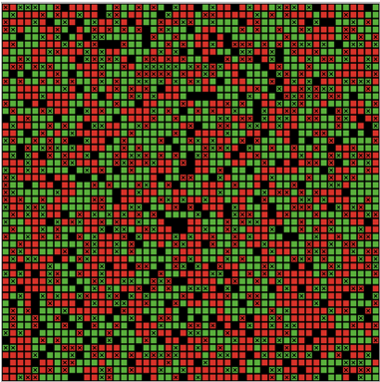
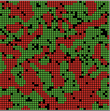
Schelling’s models illustrate the idea that slight individual behaviours or preferences can lead to aggregate results that the individuals did not intend. Schelling’s models show how a small individual preference to not be a racial minority in a neighbourhood leads to neighbourhood segregation (Schelling 1971). Figures 1a and 1b illustrate the segregation of two groups of agents resulting from a Schelling type model in Netlogo. Figure 1a is the starting point of the model with no clustering or segregation and Figure 1b is the ending point of the model where distinct clusters of agents have formed.
Schelling’s results have proven to be robust with many other researchers recreating and expanding on his work. Stoica & Flache (2014) create a model that extends the idea of residential segregation to school segregation with families picking schools based on both distance and the existing racial mix at the school. Muldoon et al. (2012) investigate the effects changing the utility function or the agents’ preferences have on the final segregation of the model. They found that even under conditions where agents prefer to be in a small minority, segregation still occurs when agents have partial information about their surroundings. Survey data showing real preferences for neighbours has been used to show that while different groups have different preferences for neighbourhood make-up, the real world preferences can be used in a Schelling segregation model that produces the results Schelling predicted (Clark 1991).
However, real world neighbourhoods are more complicated with other factors than race. For example, in looking at the household survey data, Clark (1991) note that white households will not discriminate against a number of equal status black households, showing that people not only take race into account but other factors such as income and education as well. Clark & Fossett (2008) assert that other factor such as multiple ethnic groups, socioeconomic status, and urban and demographic conditions are needed to truly understand and investigate residential patterns. These factors are not included in Schelling’s model. Even when only one factor is considered, a constant tolerance level, which is often used in Schelling type models, is unrealistic. For example, Benenson et al. (2009) use surveys to investigate cases of wealthier households in poor neighbourhoods and find that these wealthier households do not discriminate against their less wealthy neighbourhoods. In some cases there are advantages of the poorer neighbourhoods such as lower house prices.
As the Schelling segregation model only considers a world with simplified features, work has been done to expand the Schelling model to include other factors that influence neighbourhood selection. Fossett (2011) includes not only race in his model but socioeconomic status as well, giving agents preferences for housing quality, neighbourhood socioeconomic status and neighbourhood ethnic mix. Benenson et al. (2009) use tolerance to different income levels as an agent variable in their model and allow it to change with the household when modelling the segregation in Israeli cities.
Assessing the Degree of Clustering by Socioeconomic Status in Irish Towns
To determine if it is necessary to adjust a model for clustering by socioeconomic status we first must determine if there is evidence of the phenomenon in Ireland. We do not have data of the exact locations where individuals of different socioeconomic statuses live. However, the Property Services Regulatory Authority provides records in the Residential Property Price Register on the price of properties sold by address from 2010 to the present day (PSRA 2012). The Residential Property Price Register provides information including the date of sale, address, county and price [1].
Over the past few years there has been emerging literature showing the relationship between property value and socioeconomic status (Coffee & Lockwood 2012). Moudon et al. (2011) found that neighbourhood wealth measures such as property values had the potential to replace area-level socioeconomic status measures. Coffee & Lockwood (2012) found that a relative location factor based on property value can be used as a proxy for socioeconomic status. Their study determined this factor can be used to enhance area level measures and identify groupings within a given area. If we can consider house price as a proxy for socioeconomic status then it should be possible to determine if clusters of households of the same socioeconomic status exist in Ireland using the data.
Residential property price register data
For the purpose of finding clusters within the Residential Property Price Register we split the data into six sub-sets by the sale price of the house. The first subset has the houses with prices in the lower 16.67% , the second subset has houses from the second 16.67% and so forth. Table 1 shows the breakdown of prices for each subset of the dataset.
| Group | Price Range |
| Housing Group 1 | < 73,000 |
| Housing Group 2 | ≤ 73,000 and < 120,000 |
| Housing Group 3 | ≤ 120,000 and < 165,000 |
| Housing Group 4 | ≤ 165,000 and < 225,000 |
| Housing Group 5 | ≤ 225,000 and < 320,000 |
| Housing Group 6 | ≤ 320,000 |
The entire data set was then geocoded using QGIS (2009) so that it could be loaded into Netlogo (Wilensky 1999a).
Calculating dissimilarity in Irish towns
To determine the level of clustering that exists in a given region the dissimilarity index is used. The dissimilarity index is a measure that determines the “evenness" of a population or the differential distribution of social groups within a region which is composed of a set of areal units. It is a popular measure to determine the level of segregation in a space. The dissimilarity index is presented by Massey & Denton (1988) as one of the main measures to determine segregation. It is also used by the US Census Bureau in determining levels of segregation (Iceland et al. 2002). For the calculation of the dissimilarity index of a region the region is broken up into smaller spatial units call areal units. If any group is segregated then that group will be unevenly distributed. The index produces a value between 0 and 1. The closer the value to 0 the more even and less segregated a region is and the closer the value is to 1 the less even and more segregated a region is. The dissimilarity index is calculated as:
| $$D = \sum\limits_{i=1}^n \frac{t_{i}|p_{i}-P|}{2TP(1-P)}$$ | (1) |
where \(n\) is the number of areal units in the region the index is being calculated for, \(t_{i}\) is the number of households in areal unit \(i\), \(p_{i}\) is the proportion of minority households in areal unit \(i \), \(T\) is the total number of households in the region and \(P\) is the proportion of minority households across the whole population of the region (Massey & Denton 1988).
As our model is run on Irish towns we calculated the dissimilarity index for two towns that we have used our model for, Schull a small town in West Cork and Tramore a town in Waterford. Schull has a population of under 1,000 and Tramore has a population of about 10,000. As the Residential Property Price Register data has only 29 houses sold in Schull and 166 sold in Tramore between January 2010 and February 2017, the dissimilarity index was also calculated for Cork and Waterford cities to determine if the low numbers of houses sales in our target towns affected the dissimilarity index.
To calculate the dissimilarity index for each town, we break the Netlogo environment up into square grids. This is done by selecting a set of patches that will be the center of each square grid in Netlogo. Then the radius function in Netlogo is used to select patches within a radius of 5 and 10 units of each center patch (1 unit equals 1 patch in the Netlogo environment and approximately 111 m\(^{2}\) in the real environment being simulated). The radius of 5 produces areal units of 10 x 10 patches and the radius of 10 produces areal units made up of 20 x 20 patches. The square grids become our \(n\) areal units. As we are exploring the effects of clustering on the model we use two different radii to determine how the size of the areal units affects clustering. Because the house price group that is in the minority might vary between towns, for each town the dissimilarity in that unit is calculated for each house price group. For example, for the house in the first range \(p_{i}\) becomes the proportion of households in that unit that are in the same price range and \(P\) is the total proportion of households in the same price range.
Table 2 shows the dissimilarity index for the two towns and two cities calculated with a radius of 5 and 10 units. We investigated a number of other radii but only present results for two as we found a similar patterns and results for all radii. It can be seen from the table that the dissimilarity index for Tramore is similar to that for Waterford. Although there are some differences between the dissimilarity indices they are within a range that could be explained by different make ups in the towns. Schull, however, has larger differences in the less than e95,000 range and the e95,000 to e165,000 range. This is likely to the limited number of houses in the data set in those ranges. The dissimilarity indices for the towns based on house price data will be used as a benchmark to compare the dissimilarity indices for our simulated towns based on socioeconomic status in order to determine if randomly allocating agents to locations within a small area creates an appropriate distribution of agents by socioeconomic status in the towns.
Modelling Irish Towns
This work is part of a larger project that is building large scale, high fidelity agent-based models of Irish towns for epidemiological simulation. This section describes how these models are setup using publicly available datasets, and compares the dissimilarity index scores measured in the models of the towns Schull and Tramore with those calculated based on the PSRA. We then describe how the inclusion of a segregation model following Shelling changes this. Schull and Tramore are chosen as they are two towns in Ireland where concentrated measles outbreaks occurred. In 2012 there were at least 30 confirmed cases of measles in Schull in one outbreak (Corner et al. 2012) and in 2013 there were approximately 20 confirmed cases of measles in Tramore in one outbreak (O’Connor et al. 2016).
Calculating dissimilarity in the Basic Town Model
Our initial model is based on the model presented in Hunter et al. (2016), which was designed to model the spread of an infectious disease in an Irish town using only openly available data[2]. The model utilizes small area data from the central statistics office to populate the town being modeled with agents (CSO 2014). To populate the model the number of households in each small area are added into the town and randomly placed throughout the small area. Households are assigned a household type (single, couple, couple plus others, couple with children, single parent, or other), adult agents are added into the households and then assigned a sex based on a probability distribution determined from CSO data. Agents are given an age based on another CSO probability distribution for their sex and small area. Children are then added into households designated as having children and given an age and sex. Agents are assigned an economic status based on age and a random selection following the distribution of economic statuses in the small area for their sex. Agents over 65 are assigned retired, children are assigned student, and other agents are assigned work, unemployed, looking for first job, sick/disabled or stay at home. In addition to the characteristics given to agents in the Hunter et al. (2016) model, we assign working agents a social class again based on CSO data. Social class is the CSO variable used to capture socioeconomic status. Agents are assigned to the classes Professional workers, Managerial and technical, Non-manual, Skilled Manual, Semi-skilled, and Unskilled. Households are then given the social class of one of the adults in the house, the adult is randomly selected from all the adults in the household. For household social class Skilled Manual and Semi-Skilled are combined into one group (Skilled/Semi-skilled) and Unskilled is combined with unemployed individuals to create the Other group. The groupings are based off of those used by Doherty et al. (2014) in their analysis on the effects of socioeconomic status on vaccination rates in Ireland. Irish vaccination data is used to determine the percentage of each age group that received vaccinations and this is adjusted based on socioeconomic status using the odds of having children vaccinated from (Doherty et al. 2014). We also included a retired grouping that was not included in the research by Doherty et al. (2014). Unoccupied households are also added into the model. The number of unoccupied households in a small area is taken from the census data and the households are randomly placed in locations in that small area. Agents with an economic status of work are given a workplace location and school locations are added into the model. Agents move between work, school and within the community. At the start of the model a set number of agents are given the status of infected. The disease model is based on an SEIR compartment model. As the infected agents move through the town they have a certain probability of infecting susceptible agents they come into contact with (Hunter et al. 2016).
| Price Range | Radius | Schull | Tramore | Waterford | Cork |
| < 73,000 | 5 | 0.250 | 0.385 | 0.359 | 0.311 |
| 10 | 0.481 | 0.319 | 0.316 | 0.259 | |
| ≤ 73,000 and < 120,000 | 5 | 0.754 | 0.644 | 0.600 | 0.535 |
| 10 | 0.592 | 0.558 | 0.419 | 0.430 | |
| ≤ 120,000 and < 165,000 | 5 | 0.846 | 0.682 | 0.626 | 0.499 |
| 10 | 0.885 | 0.529 | 0.464 | 0.351 | |
| ≤ 165,000 and < 225,000 | 5 | 0.659 | 0.573 | 0.696 | 0.532 |
| 10 | 0.511 | 0.566 | 0.514 | 0.356 | |
| ≤ 225,000 and < 320,000 | 5 | 0.584 | 0.766 | 0.782 | 0.581 |
| 10 | 0.627 | 0.682 | 0.647 | 0.445 | |
| ≤ 320,000 | 5 | 0.616 | 0.882 | 0.808 | 0.656 |
| 10 | 0.565 | 0.937 | 0.723 | 0.513 |
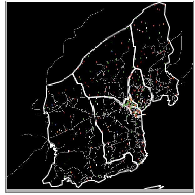
We initiate setup for our model for both Schull and Tramore 100 times (each run will be slightly different due to random initialisation) and calculate the dissimilarity index for each of the household social classes each time the model is initiated. We then find the average of the dissimilarity index across the 100 model setups. The dissimilarity index is calculated twice for each town, once using areal units with a radius of 5 and once using a radius of 10. Similar to how the dissimilarity index was calculated for the real housing price data, for each areal unit the dissimilarity in that unit is calculated for each social class. Table 3 shows the average dissimilarity index for both Schull and Tramore for each social class. Figures 2a and 2b show the initial setup of Schull and Tramore. Agents are color coded by socioeconomic status.
| Social Class | Radius | Schull | Tramore |
| Professional | 5 | 0.378 | 0.223 |
| 10 | 0.354 | 0.202 | |
| Managerial and Technical | 5 | 0.346 | 0.208 |
| 10 | 0.297 | 0.151 | |
| Non-Manual | 5 | 0.357 | 0.205 |
| 10 | 0.297 | 0.312 | |
| Skilled/Semi-skilled | 5 | 0.344 | 0.206 |
| 10 | 0.297 | 0.163 | |
| Retired | 5 | 0.346 | 0.262 |
| 10 | 0.298 | 0.263 | |
| Other | 5 | 0.359 | 0.212 |
| 10 | 0.309 | 0.168 |
Although house prices and socioeconomic status are not an exact match from the literature we can assume that house prices serve as a proxy for socioeconomic status. If randomly placing houses of different social class within a small area produces realistic neighbourhoods clustered by socioeconomic status we would expect the dissimilarity indices from the real house price data set to be similar to the dissimilarity indices from the model. Comparing the values for the dissimilarity index for each social class from the initial setup of our model to the values for the dissimilarity index for the house price ranges it can be seen that the dissimilarity indices from the simulation are generally less than those coming from the real data. As the house prices and are not similar we can conclude that even when using small area data an ABM that uses a random distribution of agents within these areas does not accurately portray neighbourhood socioeconomic status and it may be necessary to adjust the model to account for this. The only exception is the housing price range less than e95,000 in Schull has a dissimilarity index of 0.167 when a radius of 5 is used compared to values of about 0.35 for all the social classes from the simulation. The low dissimilarity index from Schull is likely due to small data samples.
Using a segregation model to better model dissimilarity
In order to account for clustering in neighbourhoods by socioeconomic status that we see in our house price data set, but not from the initial setup of the ABM, we add an additional burn-in step into our model setup process. Once the model is populated with agents and all of the agents are assigned the appropriate characteristics we give households the opportunity to move using a Schelling type segregation model. However, unlike in Schelling’s models where race is used as the segregating factor we use social class. Each household in the model has a social class assigned to it and households will seek to surround themselves with households of the same social class. To allow this households are given the opportunity to move to more attractive unoccupied houses during the burn-in process.
The model is run on discrete time steps. Each household is considered at each time step. For each household, if the proportion of neighbouring households with the same social class is below a pre-set tolerance level then the household will move to a location with more neighbouring households matching its social class. If the proportion of neighbouring households with matching social class is above the threshold the household does not move. Households moving to new locations is enabled by the inclusion of unoccupied houses in our model setup process. When a household moves they move to the unoccupied house in their current small area with the highest proportion of neighbours matching their own social class. If a better location than their current one is not available households do not move. The burn-in process stops after a time step of no households moving.
The burn-in process involves two parameters: neighbourhood size and a tolerance level for households of different social class. For neighbourhood size we use the same radii used for calculating dissimilarity (see Section 2.9): 5 units and 10 units. The next section describes experimental results that are used for setting the tolerance level.
Once the segregation model has stopped running, agents who are students are assigned to the school that is in the closest distance to their house and the disease model can be run.
Results
This section presents the results from two experiments. First we look at how the dissimilarity index for the two towns changes as we adjust the radius and tolerance of agents in the model. The second experiment determines how the clustering affects the results of the infectious disease ABM.
Using segregation modelling to model socioeconomic clustering
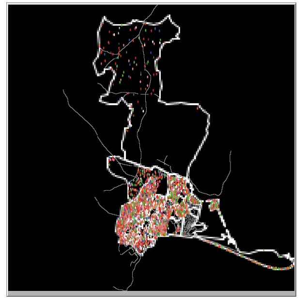
In this section we report an experiment that tested whether the use of a socioeconomic segregation model improved the calibration of an ABM in terms of making the dissimilarity index of the neighbourhoods within the model after the segregation process has been run more similar to real data than the dissimilarity index prior to the segregation model being run. In order to run a socioeconomic segregation model as part of an ABM setup process we must set 3 hyper-parameters: the number of iterations the segregation model runs for (Due to the stochastic nature of the setup, different results can be obtained each iteration or run of the model. Each iteration is a different initial setup of the model. There is a burn-in process for each iteration which runs until there no agents move in a single time step.), the tolerance level used in the model, and the radius used in the model. To explore the interactions between the hyper-parameters of the segregation model and the effect of the segregation model on the calibration of the model we: fixed the number of iteration to be 100 and set up a grid search process where tolerance took the values from 0.1 through 0.7 and the radius parameter was set to either 5 or 10. For each combination of hyper-parameters an ABM model of Schull and an ABM model of Tramore was created and a socioeconomic segregation model burn-in process was run in the burn-in process. After each iteration, the dissimilarity index for each social class within each town was calculated and stored and an average was taken across the 100 iterations. Figures 3a and 3b show the setup for Schull and Tramore after the burn-in model. Clusters of households by color can be seen in both towns, however, as Tramore has a larger population, the clusters are more distinct in Tramore.
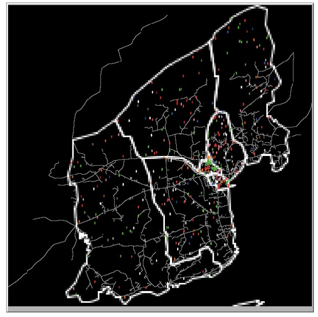
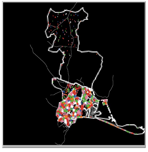
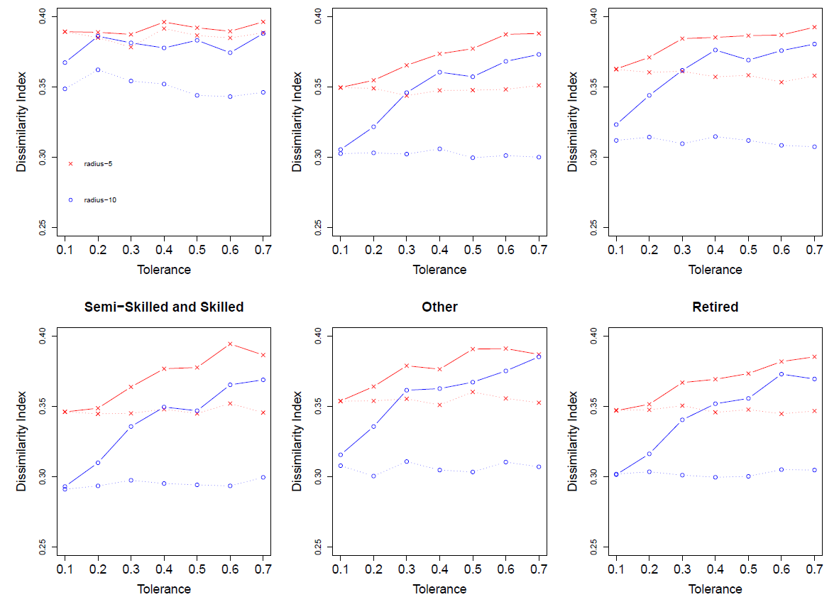
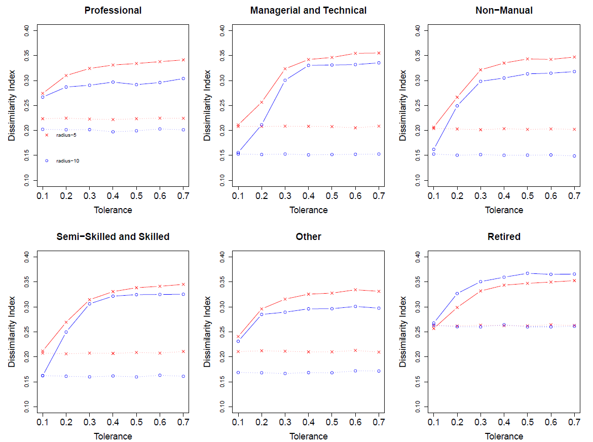
Table 4 gives the average dissimilarity index for the managerial and technical social class for each of the combinations of tolerance and radii across the 100 iterations. Comparing the final dissimilarity index for each town with the starting dissimilarity index and the real dissimilarity index based on housing price data, it can be seen that the final dissimilarity index is closer to real dissimilarity index. Although we only present the results for one of the social classes in Tables 4, Figures 4 and 5 present the results for each of the social classes for Schull and Tramore respectively. The plots in each figure show how the dissimilarity index changes as the tolerances increases. Dashed lines are the starting dissimilarity index while solid lines represent the final dissimilarity after the burn-in process. This can be seen further in Tables 5 and 6. The two tables show the starting and ending dissimilarity index for each social class in Schull and Tramore respectively. The model used to find the dissimilarity index for Tables 5 and 6 had a radius of 5 and a tolerance of 0.5.
Within a town the changes in the dissimilarity index based on tolerance and radius follow a similar pattern for each social class. However, between Schull and Tramore the differences are greater. This is likely due to the difference in size between the two towns. Tramore has ten times the population of Schull and thus more households and a greater distribution of social classes. For both towns using a radius of 5 results in higher levels of dissimilarity than a radius of 10. However, for Schull the difference between the starting dissimilarity and the dissimilarity is much greater for radius 10. As the tolerance increases for the Schull model the differences between the dissimilarity for radius 5 versus radius 10 decreases. For most social classes in the Tramore model, as can be seen in Figure 4, the difference between results from radius 5 and radius 10 tend to be smallest using a tolerance of 0.2 and 0.3 and then as the tolerance gets greater the difference increases.
Although in both towns the simulation still provides a lower value for the dissimilarity index compared to the house pricing data, we feel that the increase in value for the dissimilarity index especially for Tramore moves towards a more realistic artificial society for our simulation. The model shows it is possible to use a segregation type model as a step in the setup of an ABM to make the model more realistic. One of the factors causing the differences in clustering could have to do with the extra retired social group that we added. This was done since social class was based on employment status in our model. However, in reality the socioeconomic status of retired individuals might be based on their socioeconomic status before retirement.
| Social Class | Radius | Tolerance | Schull | Tramore |
| Managerial and Technical | 5 | 0.1 | 0.350 | 0.211 |
| 0.2 | 0.355 | 0.257 | ||
| 0.3 | 0.365 | 0.323 | ||
| 0.4 | 0.373 | 0.342 | ||
| 0.5 | 0.377 | 0.346 | ||
| 0.6 | 0.387 | 0.355 | ||
| 0.7 | 0.388 | 0.355 | ||
| 10 | 0.1 | 0.305 | 0.156 | |
| 0.2 | 0.322 | 0.211 | ||
| 0.3 | 0.346 | 0.301 | ||
| 0.4 | 0.360 | 0.330 | ||
| 0.5 | 0.357 | 0.331 | ||
| 0.6 | 0.368 | 0.332 | ||
| 0.7 | 0.373 | 0.335 |
| Social Class | Starting | Ending |
| Schull | ||
| Professional | 0.286 | 0.391 |
| Managerial and Technical | 0.347 | 0.377 |
| Non-Manual | 0.358 | 0.386 |
| Skilled/Semi-skilled | 0.345 | 0.378 |
| Retired | 0.348 | 0.373 |
| Other | 0.360 | 0.390 |
| Social Class | Starting | Ending |
| Tramore | ||
| Professional | 0.223 | 0.334 |
| Managerial and Technical | 0.208 | 0.346 |
| Non-Manual | 0.202 | 0.343 |
| Skilled/Semi-skilled | 0.209 | 0.339 |
| Retired | 0.262 | 0.347 |
| Other | 0.210 | 0.346 |
Assessing the impact of socioeconomic clustering on outbreak modelling
Although it is useful to show that the segregation model does in fact lead to a model that includes socioeconomic clustering, it is important to determine if it has an effect on our infectious disease model. If clustering agents by socioeconomic status has no effect on the results of the final epidemiological model it will not be a useful addition. In order to determine what influence the clustering has on the end results of the model, the infectious disease model was run 100 times with the socioeconomic segregation model as the final steps in setup. For the socioeconomic segregation model a radius of 5 is used with a tolerance of 0.5. The model is run for both Schull and Tramore and results are compared to model runs without clustering. Tables 7 and 8 show the summary of the results across the 100 runs for Schull and Tramore respectively.
| Schull No Clusters | Schull Clusters | |
| Minimum | 1 | 1 |
| 1st Quartile | 2 | 1.75 |
| Median | 18 | 12.5 |
| Mean | 19.57 | 16.67 |
| 3rd Quartile | 29.25 | 26.25 |
| Maximum | 68 | 84 |
| Tramore No Clusters | Tramore Clusters | |
| Minimum | 1 | 1 |
| 1st Quartile | 2 | 2 |
| Median | 79.5 | 96.4 |
| Mean | 85.97 | 110.7 |
| 3rd Quartile | 150.25 | 212.2 |
| Maximum | 322 | 497 |
Comparing the results for Schull it can be seen that the distribution of total number of infected cases is similar for both the runs with and without clustering. In fact the clustering leads to a smaller median and mean compared to results with no clusters. Tramore, however, shows a greater difference between the runs with and without clusters. With the clusters the magnitude of the outbreaks are greater. This can be further seen looking at the histograms in Figures 6 and 7. The histograms show the distribution of the number of agents infected in the outbreak. When comparing runs with and without clustering for Schull, there is a noticeable difference in runs with a small number of agents infected. Including clustering leads to an almost 10% increase in the number of runs with 0-10 agents infected in the outbreak compared to models without clustering. The Tramore distribution when clustering is included shows a higher percentage of runs with a larger number of agents infected compared to the distribution when clustering is not included.

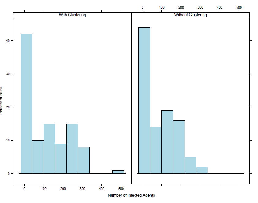
The results are not completely unexpected as Schull is a small low density town and the segregation model does not make a large difference in the level of socioeconomic clustering. For example, from Tables 3 and 4, the dissimilarity index for the managerial and technical social class with a radius of 5 is 0.346 before the segregation model and 0.377 after the segregation model. This is compared to the Tramore where the dissimilarity index before the segregation model is 0.208 and after is 0.346. Thus it makes sense that the segregation burn in model does not have much of an influence on the outcome of the infectious disease model for Schull but does have an effect on Tramore. Intuitively the greater magnitude of the Tramore outbreaks also makes sense as in the clustered Tramore model, agents with similar vaccination rates are living closer together and thus interacting more leading to more infections. Since students choose the closest schools to their home that should also lead to increased infections if students with the lower vaccination rates due to their socioeconomic status attend the same schools. As Tramore has multiple schools for students to attend while Schull only has one primary and one secondary school this could also be a factor as to why there is less of a difference between the Schull runs. The increase in the number of runs with smaller outbreaks in the Schull model with clustering could be a result of the clustering leading to communities within Schull with a higher overall vaccination rate resulting in the outbreak ending sooner in those communities due to a lack of susceptible individuals. The results show that the socioeconomic segregation model can have an effect on the outcome of the model.
Conclusion
Our model successfully used a segregation model to create more realistic distribution of socioeconomic status within small areas in order to setup our ABM. Through using house price data we determined that clusters by socioeconomic status exist in Ireland and that by randomly placing households within a small area we did not capture the correct level of clustering. Not having the appropriate mix of socioeconomic status could have an effect on an infectious disease model as the overall neighbourhood health and vaccination level of a neighbourhood has an effect on individual health.
Not only have we shown that we can use a segregation model as a step in the setup of our ABM for infectious diseases but we have determined that clusters of individuals by socioeconomic status can have an effect on the outcome of the overall model. While Schull does not show this effect, we believe this is due to characteristics of the town. A small town with less than 1,000 residents may not have enough of a sample of individuals in different socioeconomic groups for clustering to make a difference. In addition, we feel that the school settings should have a large impact on the results of the model. If a school is located in an area that has lower vaccination rates an infectious disease might spread through the school quicker than if there was an equal distribution of vaccination rates within the school. As there is only one primary and one secondary school in Schull the distribution of vaccination rates will not change regardless of the level of clustering. The increased magnitude of outbreaks in the Tramore runs lead to the conclusion that socioeconomic clustering can result in a different outbreak pattern. Tramore has a much greater population that Schull, with just under 10,000 residents allowing more distinct cluster of agents by socioeconomic status to form and allowing the spatial distribution of agents to contribute to the model results. Thus leading to the conclusion that socioeconomic distribution should be considered as a factor in an agent-based model for infectious diseases.
More work can be done to investigate how a different radius or tolerance will affect the results of the model and how the results from other towns besides Schull and Tramore are influenced by including clustering. Other extensions to the model could include running something similar to the segregation model but with workplaces. Agents are currently randomly assigned to work places without regard to social class. A segregation model for work assignment could make a more realistic ABM. In addition as both towns are small future work should focus on the feasibility of scaling the burn-in to larger towns and cities and how socioeconomic clustering might be different or have a different influence on outbreaks in a denser population.
It is impossible to make a direct comparison between the house price data set, used to determine if clustering exists, and the simulated socioeconomic data set due to data availability. The data desired to create a model is not always available. For example, while we can find house prices for sold houses we do not know the characteristics of the individuals living in those houses. In addition, we have information on individual characteristics but not have their house prices or exact location. We feel that to move forward in the field of ABMs it is necessary to take limited data and use assumptions, such as the comparison between house prices and socioeconomic status, to fill in the gaps of available data.
In addition, it should be noted that while the dissimilarity index is a measure commonly used to determine the level of clustering, it has some disadvantages. It is measured using non overlapping areal units and clustering across areal units is not taken into account with this measure. As an initial exploration into clustering within small areas, and because we are looking for clustering within and across the small areas (each small area has an accurate distribution of households by socioeconomic status before the burn-in model) we feel that the measure gives an acceptable comparison of the clustering before and after the burn-in. However, further work can be done using other spatial methods of clustering such as autocorrelation that might prove the results more robust.
Acknowledgements
This work was partly supported by the Fíosraigh Scholarship Programme of the Dublin Institute of Technology.Notes
- https://www.propertypriceregister.ie/website/npsra/pprweb.nsf/page/ppr-home-en.
- The model can be found on the Netlogo website using the following link http://ccl.northwestern.edu/netlogo/models/community/town_model_burnin.
References
BENENSON, I., Hatna, E. & Or, E. (2009). From Schelling to spatially explicit modeling of urban ethnic and economic residential dynamics. Sociological Methods and Research, 37(4), 463-497. [doi:10.1177/0049124109334792]
BOBASHEV, G. V., Goedecke, D. M., Yu, F. & Epstein, J. M. (2007). A hybrid epidemic model: Combining the advantages of agent-based and equation based-approaches. Proceedings of the 2007 Winter Simulation Conference, (pp. 1532–1537).
BRUCH, E. & Atwell, J. (2015). Agent-based models in empirical social research. Sociological Methods & Research, 44(2), 186–221. [doi:10.1177/0049124113506405]
CLARK, W. A. V. (1991). Residential preferences and neighborhood racial segregation: A test of the Schelling segregation model. Demography, 28(1), 1-19.
CLARK, W. A. V. & Fossett, M. (2008). Understanding the social context of the Schelling segregation model. PNAS, 105(11), 4109-4114. [doi:10.1073/pnas.0708155105]
COFFEE, N. & Lockwood, T. (2012). The property wealth metric as a measure of socioeconomic status. 18th Annual PRRES Conference: http://www.prres.net/papers/coffee_property_wealth_metric_for_se_status.pdf.
CORNER, S., Ryan, F., MacSweeney, M., Coughlan, H. & Kieran, M. (2012). Measles outbreak West Cork May 2012. Epi-Insight: http://ndsc.newsweaver.ie/epiinsight/dllmrzt7dc0?a=1&p=24661425&t=17517774.
CSO (2014). Census 2011 boundary files. Central Statistics Office: http://www.cso.ie/en/census/census2011boundaryfiles/.
DOHERTY, E., Walsh, B. and O'Neill, C. (2014). Decomposing socioeconomic inequality in child vaccination: Results from Ireland. Vaccine, 32(27), 3438-3444. [doi:10.1016/j.vaccine.2014.03.084]
ENDRICH, M. M., Blank, P. R. & Szucs, T. D. (2009). Influenza vaccination uptake and socioeconomic determinants in 11 European countries. Vaccine, 27(30), 4018-24.
FOSSETT, M. (2011). Generative models of segregation: Investigating model-generated patterns of residential segregation by ethnicity and socioeconomic status. Journal of Mathematical Sociology, 35(1-3). [doi:10.1080/0022250X.2010.532367]
GILBERT, N. (2008). Agent-Based Models. 7-153. London: Sage Publications, Inc.
HEGSELMANN, R. (2017). Thomas C. Schelling and James M. Sakoda: The intellectual, technical, and social history of a model. Journal of Artificial Societies and Social Simulation, 20(3), 15: https://www.jasss.org/20/3/15.html [doi:10.18564/jasss.3511]
HUNTER, E., Mac Namee, B. & Kelleher, J. D. (2017). A taxonomy for agent-based models in human infectious disease epidemiology. Journal of Artificial Societies and Social Simulation, 20(3), 2: https://www.jasss.org/20/3/2.html [doi:10.18564/jasss.3414]
HUNTER, E., Namee, B. M. & Kelleher, J. (2016). An open data driven epidemiological agent-based model for Irish towns. In Proceedings of the 24th Irish Conference on Artificial Intelligence and Cognitive Science: http://ceur-ws.org/Vol-1751/AICS_2016_paper_24.pdf
ICELAND, J., Weinberg, D. H. & Steinmetz, E. (2002). Racial and ethnic residential segregation in the United States: 1980-2000. Census 2000 Special Reports: US Census Bureau.
JESSOP, L. J., Murrin, C., Lotya, J., Clarke, A. T., O’Mahony, D., Fallon, U. B., Johnson, H., Bury, G., Kelleher, C. C. & Murphy, A. W. (2010). Socio-demographic and health related predictors of uptake of first MMR immunisation in the Lifeways Cohort Study. Vaccine, 28(38), 6338-43. [doi:10.1016/j.vaccine.2010.06.092]
MACKENBACH, J. P., Meerding, W. J. & Kunst, A. E. (2007). Economic implications of socio-economic inequalities in health in the European Union. Tech. rep., Health and Consumer Protection Directorate-General, Department of Public Health, Rotterdam, The Netherlands.
MASSEY, D. S. & Denton, N. A. (1988). The dimensions of residential segregation. Social Forces, 67(2), 281-315. [doi:10.1093/sf/67.2.281]
MOUDON, A., Cook, A., Ulmer, J., Hurvitz, P. & Drewnowski, A. (2011). A neighborhood wealth metric for use in health studies. American Journal of Preventive Medicine, 41(1), 88-97.
MULDOON, R., Smith, T. & Weisberg, M. (2012). Segregation that no one seeks. Philosophy of Science, 79(1), 38-62. [doi:10.1086/663236]
O’CONNOR, B., Cotter, S., Heslin, J., Lynam, B., McGovern, E., Murray, H., Parker, G. & Doyle, S. (2016). Catachin measles in an appopriately vaccinated group: A well-circumscribed outbreak in the south east of Ireland, September-November 2013. Epidemiology and Infection, 144(15), 3131-3138.
PSRA (2012). Residential property price register. Property Services Regulatory Authority: http://www.psr.ie/website/npsra/npsraweb.nsf/page/index-en.
QGIS (2009). QGIS geographic information system 2.8. Open Source Geospatial Foundation: http://www.qgis.org/en/site/index.html.
SCHELLING, T. C. (1969). Models of segregation. The American Economic Review, 59(2), 488-93.
SCHELLING, T. C. (1971). Dynamic models of segregation. Journal of Mathematical Sociology, 1(2), 143-186.
STOICA, V. I. & Flache, A. (2014). From Schelling to schools: A comparison of a model of residential segregation with a model of school segregation. Journal of Artificial Societies and Social Simulation, 17(1) 5: https://www.jasss.org/17/1/5.html. [doi:10.18564/jasss.2342]
WHEATON, W. D., Cajka, J. C., Chasteen, B. M., Wagener, D. K., Cooley, P. C., laxminarayana Ganapathi, Roberts, D. J. & Allpress, J. L. (2009). Synthesized population databases: A US geospatial database for agent-based models. RTI International.
WILENSKY, U. (1999a). Netlogo. Center for Connected Learning and Computer-Based Modeling, Northwestern University. Evanston, IL: https://ccl.northwestern.edu/netlogo/.
WILENSKY, U. (1999b). Netlogo segregation model. Center for Connected Learning and Computer-Based Modeling, Northwestern University, Evanston, IL.