
Introduction
Agent-based models (ABMs), by their nature, are capable of producing a rich variety of model outputs driven by a potentially large set of model (input) parameters. Revealing the relationship between these model inputs and output(s) (e.g., What is the effect of an increase in a specific parameter on the model output?) is one of the key steps to gain insight into dynamic problems with the help of the simulation model (Alam et al. 2004; ten Broeke et al. 2016). The first and most straightforward way of revealing this relationship is manual model exploration, which is guided by the modeler’s insights. Apart from introducing a sense of subjectiveness, this approach is also time-consuming especially if the model is highly-dimensional and dynamically rich. An analyst/expert on the problem domain may help to reduce the required time for exploration by focusing on the relevant subsets of the input domain which may potentially yield desired outputs. Nevertheless, some of the most interesting parts of the output space may still be unexplored (Lee et al. 2015).
Systematic and automated model exploration approaches which eliminate the disadvantages of human-guided methods comprise sampling techniques from the design of experiments (DoE) literature and soft computing techniques including meta-heuristic approaches and machine learning. However, DoE techniques are not directly applicable for many ABMs since these methods assume that errors are normally distributed and existing relationships between inputs (model input parameters) and output are low-order and linear. Besides, DoE methods require many simulation runs to precisely estimate the effects of inputs (and their interactions) on the model output when the number of inputs is high (Sanchez & Lucas 2002; Kleijnen & Van Beers 2004; Lorscheid et al. 2012; Lee et al. 2015). In addition, higher-order interactions among input parameters and some special characteristics of ABMs such as tipping point behavior, adaptation and path dependency also imply potential highly nonlinear relationships between model inputs and outputs, which may further violate the assumptions of DoE-based techniques (Wilensky & Rand 2015; ten Broeke et al. 2016). Another useful approach for the analysis of ABMs is meta-heuristic techniques. However, meta-heuristic techniques are “prescriptive” rather than “descriptive”; instead of exploring the input space of an ABM comprehensively, they are useful for parameter tuning/model calibration/sensitivity analysis (Calvez & Hutzler 2006; Stonedahl & Wilensky 2010a; Stonedahl & Rand 2014; Chica et al. 2017; Moya et al. 2017) and finding parameter combinations that yield specific ABM behavior (e.g., vee formation) (Stonedahl & Wilensky 2010b). Although meta-heuristics effectively reduce the computational burden of search in input space, they still need simulation model evaluation to find the parameters that fit the objective of the analyst. In addition to these techniques, the machine learning domain also offers a broad set of potentially useful tools for the analyst for exploration. Among these, supervised learning algorithms aim to build a mapping (e.g., a functional relationship) from simulation model inputs to the outputs based on input-output data obtained from the simulation model (Alpaydin 2014). The resulting function can be considered as a representation of the original simulation model.
In this respect, a metamodel is as an approximate and a simpler representation of the input-output relationship of a simulation model (Kleijnen & Sargent 2000; Kleijnen et al. 2005). Rather than analyzing a simulation model, working on its metamodel has two main advantages: First, if the metamodel is a good representation (i.e., accurate enough to replace the original model), the analyst can rely on estimated outputs as an alternative to running the original simulation model and generating exact outputs. This reduces the required time for certain steps in the modeling cycle such as policy/scenario analysis and testing, especially when simulation run times are significant. Instead of evaluating each parameter combination in the “expensive” simulation model for exact outputs, the analyst can obtain estimates in a relatively short time. Considering complex ABMs with large sets of inputs and the need for replication to obtain reliable results, developing a compact version of the original model is beneficial. Second, if the constructed metamodel is interpretable[1] (i.e., it leads to a better understanding of input-output relationships), it can give insights into the dynamic problem by depicting how the model parameters affect the output individually and together. However, accuracy and interpretability of metamodels (and supervised learning techniques in general) are two conflicting objectives; most of the techniques which yield accurate models generate also very complex models with low interpretability and techniques yielding highly interpretable models also lacks accuracy (Lou et al. 2012; Lakkaraju et al. 2016).
Metamodeling techniques have been implemented on discrete-event (Kilmer et al. 1997; Can & Heavey 2012) and system dynamics models (Kleijnen 1995; Alam et al. 2004) to reduce run times and gain insights into the simulation model. However, most of these metamodels are limited to first- and second-order linear regression models (e.g., Madu 1990; Aytug et al. 1996; Durieux & Pierreval 2004; Kleijnen et al. 2005). Although regression methods are interpretable and easy to construct, they may not be suitable as a representation for highly nonlinear simulation models since the number of coefficients to be estimated and the required data for this estimation increase dramatically if higher order terms and interactions are added to the model (Jin et al. 2001). Considering these limitations, many researchers have been using different methods for metamodel development, including neural networks (Hurrion 1997; Kilmer et al. 1997; Badiru & Sieger 1998), kriging (Garcet et al. 2006; Chen et al. 2012; Cadini et al. 2015), multivariate adaptive regression splines (Friedman 1991; Bozağaç et al. 2016) and support vector regression (Pan et al. 2010; Zhu et al. 2012; Zhou et al. 2015).
Although metamodeling has potential advantages such as insights into input-output relationships and reduced runtimes for agent-based modelers and analysts, there are only introductory-level studies in the literature (e.g., Ipekci 2002; Yau 2002; Kleijnen et al. 2005; Happe et al. 2006). Therefore, we present a machine learning-based metamodeling approach to approximate the input-output relationship of ABMs and show how the resulting metamodel can be used to generate rule sets, which increase the understanding of the relationship between simulation model inputs and output-of-interest. For demonstrative proposes, we apply the proposed approach on the well-known Traffic Basic model (Wilensky 1997). Furthermore, we provide an R (R Core Team 2017) script that implements the presented metamodeling and analysis work flow. This script, which is given as an electronic supplement to this article, makes the reported process repeatable on other ABMs.
The proposed approach is based on support vector regression, which is chosen since (i) it is capable of approximating highly nonlinear systems (Zhu et al. 2009, 2012) and (ii) it outperforms approaches such as neural networks, kriging, multivariate adaptive regression splines in terms of accuracy and robustness[2] (Clarke et al. 2005; Li et al. 2010). However, the interpretability of support vector regression models is limited especially when handling nonlinearity. Therefore, we utilize decision trees to understand how support vector regression technique generates predictions for different parameter combinations. This coupled use of SVR and decision trees is a novel implementation that provides accurate metamodels with interpretability.
The purpose of this paper is threefold: (i) to present a model analysis tool that utilizes SVR and decision trees to analyze input-output relations of a model. The tool is implemented in R and ready available to be used in conjunction with NetLogo models, (ii) to demonstrate the technical background and implementation details of the proposed tool, and apply it on a sample ABM for demonstrative purposes, (iii) to discuss the potential uses of such a tool in specific, and metamodels in general.
The remainder of this paper is organized as follows: First, we give brief background information on support vector regression (SVR). The experimental procedures that are followed to lay down the potential merits and problems of SVR-based metamodeling are introduced in detail in Section 3. The subsequent section is devoted to experimental results, and the rule extraction procedure. In the last section, we summarize our main insights regarding SVR-based metamodeling approach and their potential contribution to the toolbox of agent-based modeling community.
Support Vector Regression
As already mentioned, metamodeling techniques can help the analyst to capture the relationship between simulation model inputs and outputs by constructing a mapping. However, one needs training data, which consists of a set of features (\(x\)) and outputs (\(y\)) associated with these features, to learn the mapping. In this study, we utilize support vector regression (SVR) as the metamodeling technique. The SVR metamodel is trained on a dataset consisting of a set of simulation model inputs (as features) and corresponding simulation model outputs.
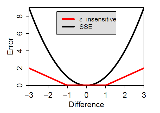
Support vector regression (SVR) is a modified version of support vector machine (SVM) classification technique for predicting continuous outputs. Most regression techniques incorporate sum of squared error (SSE) function to quantify the difference between real (\(y\)) and predicted (\(\hat{y}\)) values. However, in SVR setting, the error measure is \(\varepsilon\)-insensitive loss function (Alpaydin 2014):
| $$E_{\varepsilon}(y_{i}, \hat{y}_{i}) = \left\{ \begin{array}{ll} 0 & \quad if \quad |y_{i} - \hat{y}_{i}| < \varepsilon \\ |y_{i} - \hat{y}_{i}| - \varepsilon & \quad otherwise \end{array} \right. $$ | (1) |
Unlike SSE function, which is \(E(y_{i}, \hat{y}_{i}) = \sum_{i=1}^N \left( y_{i} - \hat{y}_{i} \right)^2 \), \(\varepsilon\)-insensitive loss function ignores errors less than \(\varepsilon\). Besides, the effect of errors greater than \(\varepsilon\) is linear. Therefore, SVR models are more robust to noise (Hastie et al. 2009; Alpaydin 2014). The difference between the sum of squared error (SSE) and \(\varepsilon\)-insensitive loss function is shown in Figure 1.
Assume that we have a training data \(\left( \boldsymbol{x}_{1}, y_{1} \right), \ldots, \left( \boldsymbol{x}_{N}, y_{N} \right) \) of size \( N \), where \( \boldsymbol{x} \) denotes the (simulation) input vector[3] and \(y\) denotes the resulting (simulation model) output. SVR aims to approximate the relationship between inputs and outputs by constructing a function (e.g., \( f\left( \boldsymbol{x} \right) = \langle \boldsymbol{w}, \boldsymbol{x} \rangle + b\)) and is formulated as a convex optimization problem as follows (Vapnik 1995; Smola & Schölkopf 2004),
| $$\begin{matrix} \displaystyle \min_{\boldsymbol{w}, b, \xi_{i}^{+}, \xi_{i}^{-}} & \displaystyle \frac{1}{2}\|\boldsymbol{w}\|^2 + C \sum_{i=1}^N \left( \xi_{i}^{+} + \xi_{i}^{-} \right) \\ \\ \textrm{subject to} \\ & y_{i} - \langle \boldsymbol{w}, \boldsymbol{x}_{i} \rangle - b \leq \varepsilon + \xi_{i}^{+} & i = 1, \ldots, N \\ \\ & \langle \boldsymbol{w}, \boldsymbol{x}_{i} \rangle + b - y_{i} \leq \varepsilon + \xi_{i}^{-} & i = 1, \ldots, N \\ \\ & \xi_{i}^{+}, \xi_{i}^{-} \geq 0 & i = 1, \ldots, N \\ \\ & \boldsymbol{w}, b, unrestricted \end{matrix}$$ | (2) |
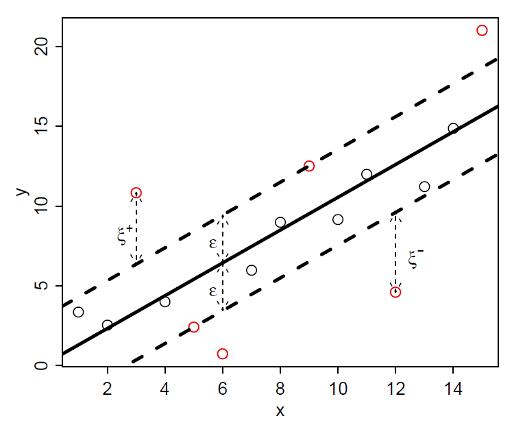
The solution of the dual of the problem given above shows that, for all points inside the \(\varepsilon\)-tube (i.e., the area between the two dashed lines in Figure 2), we have \(\alpha_{i}^{+} = \alpha_{i}^{-} = 0\). The points on the boundary or the outside of the \( \varepsilon \)-tube are called support vectors (red circles in Figure 2) and they satisfy either \(\alpha_{i}^{+} > 0\) or \(\alpha_{i}^{-} > 0\). The regression function is defined as a linear combination of support vectors[4] using Equation 10 (Alpaydin 2014):
| $$f\left( \boldsymbol{x} \right) = \langle \boldsymbol{w}, \boldsymbol{x} \rangle + b = \sum_{i=1}^N \left( \alpha_{i}^{+} - \alpha_{i}^{-} \right) \langle \boldsymbol{x}_{i}, \boldsymbol{x} \rangle + b $$ | (3) |
In this setting, the relationship between inputs and outputs is approximated by a linear function (Equation 3). To extend this formulation to handle nonlinearity, the dot product in Equation 14, \( \langle \boldsymbol{x}_{i}, \boldsymbol{x}_{j} \rangle\), is replaced by kernel functions, \( K\left(\boldsymbol{x}_{i}, \boldsymbol{x}_{j} \right)\). Some of the most frequently used kernel functions are as follows (Hastie et al. 2009; Alpaydin 2014):
- Polynomials of degree \(p\):
$$K\left(\boldsymbol{x}_{i}, \boldsymbol{x}_{j} \right) = \left( 1 + \langle \boldsymbol{x}_{i}, \boldsymbol{x}_{j} \rangle \right)^p$$ (4) - Radial basis functions:
$$K\left(\boldsymbol{x}_{i}, \boldsymbol{x}_{j} \right) = exp\left( -\gamma \|\boldsymbol{x}_{i} - \boldsymbol{x}_{j}\| ^2 \right) $$ (5) - Sigmoidal functions:
| $$K\left(\boldsymbol{x}_{i}, \boldsymbol{x}_{j}\right) = tanh\left( 2 \langle \boldsymbol{x}_{i}, \boldsymbol{x}_{j} \rangle + 1 \right)$$ | (6) |
In this study, we use radial basis kernel because it allows us to approximate both linear and sigmoid kernel under certain conditions and has some numerical and computational advantages over linear and sigmoid kernels (e.g., polynomial kernels can go to zero or infinity when \(p\) is large) (Hsu et al. 2003; Keerthi & Lin 2003). Furthermore, it yields highly accurate prediction models (Wang et al. 2003) and therefore, it is more commonly used by researchers compared to other kernel functions (e.g., Clarke et al. 2005; Zhu et al. 2009; Pan et al. 2010).
After replacing the dot product by a kernel, the regression function is
| $$f\left( \boldsymbol{x} \right) = \sum_{i=1}^N \left( \alpha_{i}^{+} - \alpha_{i}^{-} \right) K\left(\boldsymbol{x}_{i}, \boldsymbol{x}\right) + b \label{eq:svfkernel} $$ | (7) |
Experimentation
In order to inspect the potential strengths and weaknesses of a SVR-based metamodeling approach for analyzing ABMs, we conducted an experimental study. We first selected a basic and well-known model as the experimental ground, which is introduced below. In the following subsections, we specify the details of the metamodel development and testing approach.
Example model: Traffic basic
The formation of traffic jams without any physical obstruction (i.e., phantom jam) has been extensively studied in the literature because it is an emergent behavior resulting from interactions among individual entities of the system, i.e., cars (Wilensky & Resnick 1999). An ABM by Resnick (1997) and its improved version, namely Traffic Basic (Wilensky 1997), show how traffic congestions occur without any physical blockage on the road, with a very simple system representation (Riener & Ferscha 2009). This model is a suitable test bed to show the usefulness of metamodeling given that it is nonlinear. In addition, it allows us to show the usefulness of the rule extraction to understand relationships that cannot be easily inferred from input-output data. Furthermore, it is possible to validate the extracted rules by comparing them with the results reported in the literature (e.g., Treiber et al. 2000). Therefore, we used Traffic Basic Model, which can be found in NetLogo models library (Wilensky 1999), as the experimentation ground. This model simulates the flow of cars moving on a single-lane road, and has three main parameters to be specified: (i) number of cars ([1, 41]), (ii) deceleration ([0, 0.1]), and (iii) acceleration ([0, 0.01]), all sampled uniformly from their respective intervals. An initial speed between 0.1 and 1.0 is randomly assigned to each car. Besides, the speed limit is 1.0 and the minimum possible speed is 0. At each iteration, each car decelerates if there is a car ahead and accelerates otherwise. One of the cars is randomly selected to observe the effects of the model parameters on the speed. We select the output of the model as the average speed of the randomly selected car over 1000-time steps.
Dataset generation
In the machine learning domain, the common practice is to split data in two distinct groups, i.e., a training set and a test set. The training set is used to fit a predictive model (e.g., metamodel) and to adjust its hyperparameters[5]. Then, the test set is used to evaluate the predictive performance of the trained machine learning model. Each dataset includes instances (also known as samples) having two main components: a set of features (also known as predictor variables, independent variables, attributes) (\(x\)) and the output (\(y\)) associated with these predictors.
In this study, we follow a similar procedure. We generate a training and a test set by using the selected agent-based model. The set of features for a training or test sample consist of input parameter values (\(\boldsymbol{x}\)) and the output component of the sample is simply the model output (\( y \)). In order to identify the parameter value combinations to be included in the training set, we employ maximin Latin hypercube sampling[6] (Johnson et al. 1990), which is an extension of the random Latin hypercube sampling technique (McKay et al. 1979), to ensure that the input space is evenly sampled. Maximin Latin hypercube sampling algorithm satisfies this property by maximizing the minimum distance between input sample points. Due to the stochastic nature of maximin Latin hypercube sampling, we generate 30 distinct training sets (i.e., \(T = 30\)) each of which includes 30 instances (i.e., \(N = 30\)). Besides the original simulation model inputs, we define an additional feature named ratio which is equal to acceleration divided by deceleration. As the second component of the training set (\(y\)), we report the averages of 30 replications (i.e., \(R = 30\)) as outputs for each input parameter combination. In addition to the training set, we use a comparatively larger test set which includes 500 instances. We employ simple random sampling to generate the input parameter values of the test set. Similar to the training set, we report the averages of 30 replications as outputs for each input parameter combination of the test set.
Hyperparamater optimization
SVR technique (with radial basis kernel) has three hyperparameters that must be selected by the analyst: \(C\) (penalty factor), \(\varepsilon\) (parameter of the \(\varepsilon\)-insensitive loss function), and \(\gamma\) (spread parameter of the kernel). We perform a grid search on the selected subset of hyperparameter space. For each hyperparameter combination (i.e., \(\left (C, \varepsilon, \gamma \right )\)), we perform leave-one-out cross-validation on the training set[7]. Then, the hyperparameter combination yielding the minimum cross-validation error is selected. Finally, the metamodel is trained with the selected hyperparameters and used to predict the instances on the test set. In this example, we select the hyperparameter subsets as follows: \(C = \left \{ 10^{i} | i \in [-3, 3], i \in \mathbb{Z} \right \} \), \(\varepsilon = \left \{ 10^{i} | i \in [-3, 0], i \in \mathbb{Z} \right \} \), and \(\gamma = \left \{ 10^{i} | i \in [-3, 3], i \in \mathbb{Z} \right \} \).
Performance Evaluation
The main performance criteria for metamodel evaluation is Root Mean Square Error (RMSE),
| $$RMSE = \sqrt[]{\sum_{i=1}^{N} \frac{\left ( \hat{y}_{i} - y_{i} \right )^2}{N}}$$ | (8) |
Numerical Results
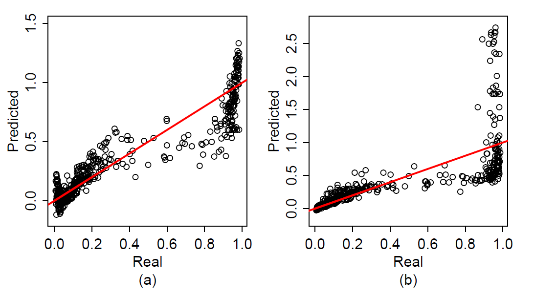
As we mentioned above, we generate 30 distinct training sets (\(T = 30\)) and then we fit a metamodel using each one of these training sets. By doing so, we aim to observe variations in the performance of the approach in response to changes due to sampling-rooted randomness in the training set to be used. Then, we evaluate the performance of these metamodels on a single test set. The average RMSE over 30 metamodels is 0.1881 with a standard deviation of 0.0503. Besides, when we inspect the individual performance of metamodels based on the best and worst training sets, the minimum and maximum RMSE values are 0.1396 and 0.3449, respectively. Figure 3 shows simulated output values (\(x\) axis) vs their predicted values (\(y\) axis) obtained with the SVR models yielding the lowest and the highest RMSE values. In both subfigures, the red line represents \(y = x\) line. If predictions returned by a metamodel are sufficiently accurate, we expect that all points should lie on the red line or be very close to it.
Although the metamodels successfully predicted the lower values of simulation model outputs, they generated large prediction errors for outputs greater than 0.8. We also observed that metamodels overestimated outputs of certain instances whose outputs were close to 1 and underestimated outputs of certain instances whose outputs were close to 0. However, this did not cause a major problem since we know that original model outputs were between 0 and 1. Figure 3 also shows the output distribution of the instances in the test set. We observed that Traffic Basic model exhibits a bimodal behavior; most outputs were between 0 and 0.2, and close to 1.
Rule Extraction
Although the SVR method is successful at capturing the overall nonlinear relationship between inputs and output, it is not easy to extract and interpret the knowledge which SVR learns from the training data. If the main concern of the analyst is simply to obtain accurate predictions, interpretability may be sacrificed. However, interpretability of machine learning models increases the credibility of the predictions especially in some domains such as medical diagnosis, credit risk evaluation, and justice (Martens et al. 2007; Barakat & Bradley 2010; Lakkaraju et al. 2016). Besides the increased trust, rule extraction allows the analyst to discover patterns and regularities in the system from which the training data is collected. Therefore, there are many attempts in the literature to extract decision rules and gain insights into how the SVR prediction function generates predictions for given parameter combinations (Martens et al. 2007; Barakat & Bradley 2010).
Rule extraction techniques can be categorized into three main groups: (i) decompositional, (ii) pedagogical, and (iii) eclectic. Decompositional methods utilize the internal structure of the prediction model (e.g, support vectors, hyperplane). However, pedagogical rule extraction methods consider the prediction model as a black-box and aim to capture how the prediction function relates inputs to outputs. Eclectic techniques combine the basics of both decompositional and pedagogical methods (Martens et al. 2009; Barakat & Bradley 2010).
Here, we used a pedagogical method to extract rules from the trained SVR model. The first step in pedagogical rule extraction procedures is to predict the outputs of a set of unlabeled parameter combinations by using a complex but accurate machine learning technique. Then, these parameter combinations and associated predictions are combined to form a dataset. In the third step, a more interpretable machine learning technique (e.g., decision trees) is trained with this new dataset for rule extraction.
In our particular case, we picked the test set that is used at the former stage for evaluating the trained SVR metamodel as the starting point. Then, the original output values (the precise ones that are obtained with the Traffic Basic model) in this dataset are replaced with the predictions of the SVR metamodel in order to obtain a dataset that can be used to train a decision tree model for rule extraction. Using the test set as the basis allows us to evaluate the extracted rules. Since we have the actual output values that are associated with each parameter combination in this dataset, we can evaluate the validity of the rules easily. To be more specific, we can compare the expected model output for a certain rule with the average of observed output values for parameter combinations that obey this particular rule.
Decision trees
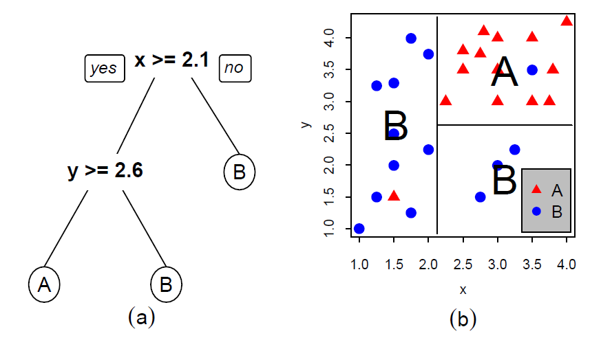
Tree-based methods are very popular machine learning techniques since they yield highly interpretable classification and regression models (Bishop 2006; Hastie et al. 2009). A decision tree iteratively partitions the input space (in our case, input parameter space of a simulation model) by generating axis-parallel splits. In each iteration, it uses only one input variable for binary splitting (Bishop 2006). This set of splits can also be visualized as a binary tree which is easy to understood (Figure 4). To label a new instance, one simply follows the path from the root to the terminal (leaf) nodes by considering each splitting rule in the intermediate nodes. For the classification tree shown in Figure 4, an unlabeled instance with \(x = 3.7\) and \(y = 2.0\) is classified as B. For a classification tree, each terminal node corresponds to the majority of the classes of the training data it includes. However, in a regression tree, terminal nodes represent the average of the numerical outputs of the training instances they include. Since we are dealing with continuous model outputs, we used regression trees in this study.
In a decision tree, a node is split into two child nodes if the impurity of that node is greater than a threshold value, which is also a tuning parameter to control the depth (complexity) of the tree. In regression, the impurity of a node is measured by the sum of squared error (SSE) (Loh 2011). One can also use some parameters such as “minimum number of instances allowed in a terminal node” or “minimum number of instances in a node to perform splitting” to control the number of splits. AID (Morgan & Sonquist 1963), GUIDE (Loh 2002), and CART (Breiman et al. 1984) are some of the algorithms proposed to construct regression trees. In this study, we employ rpart package (Therneau et al. 2015), which is an implementation of CART algorithm in R (R Core Team 2017). The computational complexity of tree training is \(O(pN\log{}N)\) where \(N\) is the number of training instances and \(p\) is the number of simulation input parameters (Hastie et al. 2009).
To transform a decision tree to a set of IF-THEN rules, one should simply trace the path from the root to each leaf node. Since each binary decision must be satisfied along the path, these decisions are combined using AND. For example, the tree in Figure 4 yields three decision rules that are shown in Table 1.
| Rule # | Rule | ||||||
| 1 | IF | x < 2.1 | THEN | class = B | |||
| 2 | IF | x≥ 2.1 | AND | y < 2.6 | THEN | class = B | |
| 3 | IF | x≥ 2.1 | AND | y≥ 2.6 | THEN | class = A |
Rule sets
As mentioned in the rule extraction section, we replaced the outputs of the instances in the test set with their predictions returned from SVR model. Then, we fitted a decision tree using this modified test set with default parameter setting in rpart package. In a sense, we tried to make the input-output mapping of the SVR metamodel more explicit by using the modified test set as the learning ground. Since the terminal node values of a regression tree are obtained by averaging the numerical outputs of the training instances they include, the rule sets derived from trees give information about traffic flow characteristics (e.g., slow or fast) rather than precise numerical values.
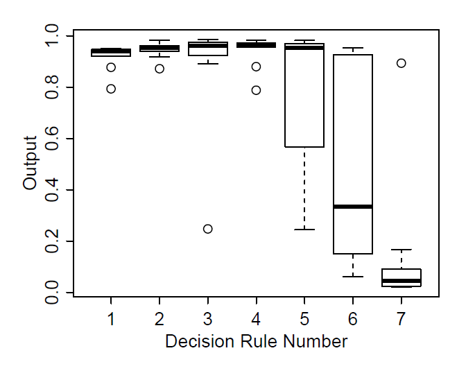
For illustrative purposes, we first fitted a decision tree on the modified test set whose outputs were obtained from the SVR model yielding minimum RMSE value (0.1396). The resulting tree is shown in Figure 5. In addition, Table 2 lists all the rules derived from the tree. We observed that, except for one intermediate node, the tree uses number of cars or ratio as splitting features making it more compact and interpretable.
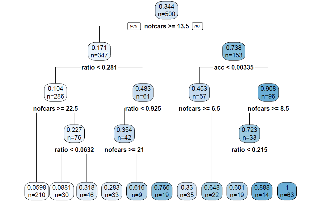
| Rule # | Rule | |||||||
| 1 | IF | nofcars < 8.5 | AND | acc ≥ 0.00335 | THEN | y = 1 | ||
| 2 | IF | 8.5 ≤ nofcars < 13.5 | AND | acc ≥ 0.00335 | AND | ratio ≥ 0.215 | THEN | y = 0.888 |
| 3 | IF | nofcars ≥ 13.5 | AND | ratio ≥ 0.925 | THEN | y = 0.766 | ||
| 4 | IF | nofcars < 6.5 | AND | acc < 0.00335 | THEN | y = 0.648 | ||
| 5 | IF | 13.5 ≤ nofcars < 21 | AND | 0.281 ≤ ratio < 0.925 | THEN | y = 0.616 | ||
| 6 | IF | 8.5 ≤ nofcars < 13.5 | AND | acc≥ 0.00335 | AND | ratio < 0.215 | THEN | y = 0.601 |
| 7 | IF | 6.5 ≤ nofcars < 13.5 | AND | acc < 0.00335 | THEN | y = 0.33 | ||
| 8 | IF | 13.5 ≤ nofcars < 22.5 | AND | 0.0632 ≤ ratio < 0.281 | THEN | y = 0.318 | ||
| 9 | IF | nofcars ≥ 21 | AND | 0.281 ≤ ratio < 0.925 | THEN | y = 0.283 | ||
| 10 | IF | 13.5 ≤ nofcars< 22.5 | AND | ratio < 0.0632 | THEN | y = 0.0881 | ||
| 11 | IF | nofcars ≥ 22.5 | AND | ratio < 0.281 | THEN | y = 0.0598 | ||
The rules derived from the tree in Figure 5 show that high number of cars and low ratio[8] values yield smaller outputs, which means slower traffic flow. In other words, high number of cars, low acceleration and high deceleration values causes traffic jam. The rules also show that low number of cars and high ratio values result in a faster traffic flow. In addition to these relatively straightforward results, the most counterintuitive observation is that, even if the number of cars is high, it is possible to obtain a fast-moving traffic if drivers speed up suddenly and slow down smoothly (see Rule 3).
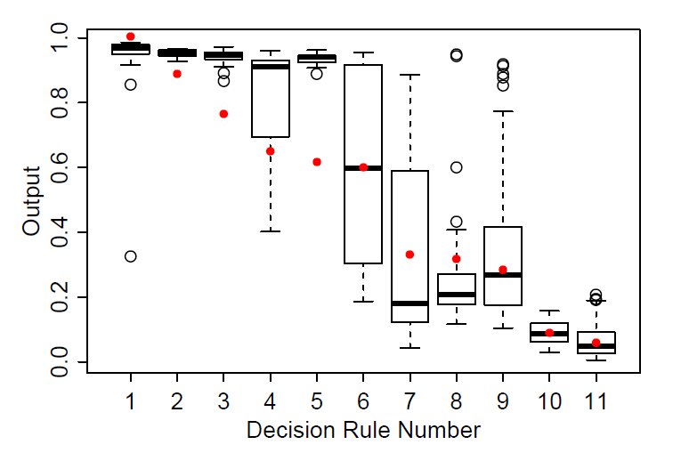
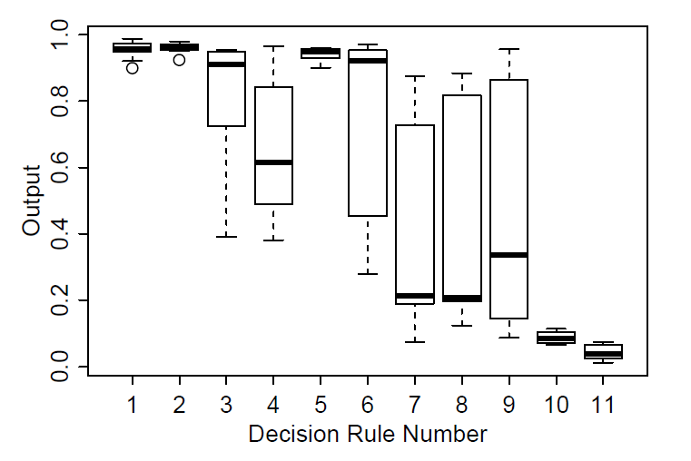
In Figure 6, solid red dots represent the output value estimated by the decision tree for input parameter combinations that satisfy the corresponding rule. In other words, these red dots represent the expected response of the SVR metamodel for a given rule. When we investigated the rules that are expected to specify high or low speed cases, the metamodel does a good job in characterizing those cases with rules 1-3 and 7-11. The metamodel deviates from the actual output in cases that are specified by rules 4-6. That can be explained by the metamodel failing to represent the transition of the model behavior from the high-speed mode to the low-speed mode. When we investigated the boxplots of the actual model output, that seemed to be normal as the actual model output demonstrated a significant variation. However, we noted that the analyst may not have a separate test set to analyze and check the original outputs of the rules. Therefore, as a further investigation to check the variability of the original simulation model outputs, the analyst can generate parameter combinations that satisfy each rule and, then, by evaluating them on the original simulation model, the analyst can generate boxplots of actual output values of these parameter combinations. For example, in Figure 7, we generated the boxplots of the actual simulation model outputs for each rule by sampling and evaluating 10 input parameter combinations (with 5 replications for each). We observed a high variability in the outputs for rules 6-9 as in Figure 6. We add this investigation to our tool as an optional step to check whether the SVR metamodel fails to capture the original simulation model behavior with high accuracy for some rules.
The second example is the decision tree that is trained on the modified test set whose outputs are obtained from the SVR model yielding maximum RMSE value (0.3449). The resulting tree is shown in Figure 8 and Table 3 lists all the rules extracted from the tree.
The rules show that high ratio values yield fast traffic flow independent from the number of cars (rules 1-3 in Table 3). In other words, independent from the number of cars on the road, traffic may flow fast if high acceleration and low deceleration values are adopted by drives. Rule 7 shows that high number of cars and low ratio values yield slower traffic flow. These conclusions are in accordance with the findings obtained from the rules extracted from the most accurate metamodel. This also shows that a metamodel with comparatively low accuracy can still provide valuable insights to the analyst.
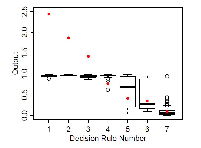
Figure 9 shows that rules 1-3 successfully specify high speed cases although SVR and decision tree models overestimates the real outputs (see solid red dots). Comparing estimated outputs of rules and actual model outputs (boxplots), we can see that rules 4 and 7 is able to point out high and low speed cases respectively. However, metamodel failed to predict the instances specified by rules 5 and 6 since the simulation model exhibited a bimodal behavior. If the analyst conducts simulation runs for parameter combinations satisfying each rule, it becomes more clear that the simulation model exhibits a bimodal behavior for the rules 5 and 6 (Figure 10).
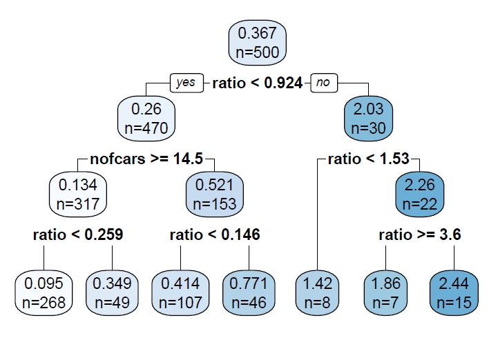
| Rule # | Rule | |||||
| 1 | IF | 1.53 ≤ ratio < 3.6 | THEN | y = 2.44 | ||
| 2 | IF | ratio ≥ 3.6 | THEN | y = 1.86 | ||
| 3 | IF | 0.924 ≤ ratio < 1.53 | THEN | y = 1.42 | ||
| 4 | IF | nofcars < 14.5 | AND | 0.146 ≤ ratio < 0.924 | THEN | y = 0.771 |
| 5 | IF | nofcars < 14.5 | AND | ratio < 0.146 | THEN | y = 0.414 |
| 6 | IF | nofcars ≥ 14.5 | AND | 0.259 ≤ ratio < 0.924 | THEN | y = 0.349 |
| 7 | IF | nofcars ≥ 14.5 | AND | ratio < 0.259 | THEN | y = 0.095 |
R Script for Metamodeling and Rule Extraction
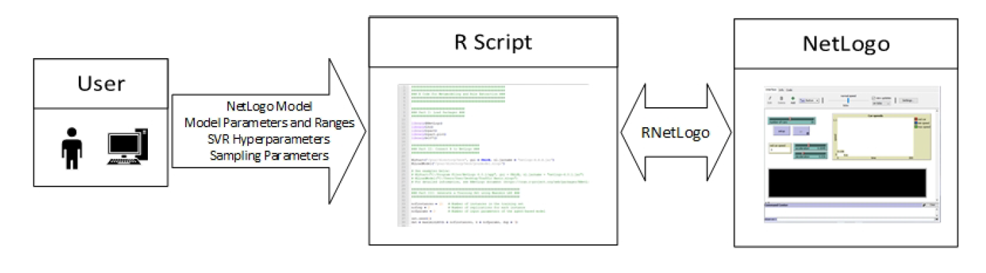
In order to increase the potential utilization of the approach by agent-based modelers and analysts, we implement it in R programming language (R Core Team 2017) and provide it as an electronic supplement[9]. The provided R script works with NetLogo models by using RNetLogo package (Thiele 2014). The analyst must only specify the NetLogo model name, model parameters and their ranges, SVR hyperparameters and sampling parameters (Figure 11). Appendix B presents a brief user guide.
Although the training set generation step of the R script (step 3 in Appendix B) is tailored to ABMs that use NetLogo as the modeling environment, the analyst can also upload a training set obtained from an ABM which uses other modeling platforms. Therefore, the analyst/user can skip training set generation step of the script and directly develop a metamodel and perform rule extraction.
The presented R script utilizes Traffic Basic model as an example. However, we add detailed comments to the code to make it applicable to other ABMs.
Conclusions
In the simulation modeling cycle, model analysis and interpretation step is crucial for understanding model dynamics and gaining insights into the dynamic problem at hand. One of the important tasks in this step is to develop an understanding about model input-output relationships. Therefore, a set of manual (i.e., human-guided) and systematic techniques are offered in the literature to ease the exploration of input-output relationship. However, human-guided techniques are prone to be biased and more systematic techniques from the design of experiment literature are mostly not capable of approximating highly nonlinear relationships, which are very common in the majority of the agent-based models. Due to their prescriptive nature, meta-heuristic techniques aim to find the parameter combinations minimizing or maximizing an objective function defined by the analyst with minimum possible model runs. Therefore, they do not perform an extensive exploration of input space of a simulation model.
Unlike these methods, supervised machine learning approaches enable us to capture the input-output relationships comprehensively by constructing a mapping from simulation inputs to outputs. This mapping function is also known as “metamodel” and can be considered as a simplified representation of a simulation model. Recent advances in machine learning allow us to develop metamodels which can capture nonlinearities embedded in a system. Therefore, we used support vector regression technique, which is proven to be successful in accurately (i.e., with small errors) approximating the underlying input-output functions of wide variety of engineering systems. To this end, we built a tool which generates a dataset and trains a support vector regression metamodel based on this dataset. We used this tool to develop a metamodel of an example agent-based model, Traffic Basic, which exhibits a bimodal behavior. Numerical results show that the metamodels perform well on average.
In support vector regression, using kernels to approximate the nonlinearities in a system results in complex regression functions with limited comprehensibility. In other words, the resulting function can be used for prediction rather than understanding the dynamics of a simulation model. Therefore, we used a rule extraction technique, which is also included in our tool, to use the metamodel not only for prediction but also as a decision/policy support tool. This rule extraction technique utilizes decision trees and generates IF-THEN rules which relate inputs to outputs and are much more interpretable compared to regression function. Rules extracted from the Traffic Basic model reveal parameter subspaces that yield low and high speed. Besides, rules obtained from the best and worst performing metamodels give some counterintuitive results about the dynamics of the model. It is possible to obtain a fast traffic flow by adjusting the ratio between acceleration and deceleration although the number of cars in a road is relatively high. These results also show that a metamodel with comparatively low accuracy still provides useful information of an agent-based model.
The coupled use of metamodeling and rule extraction presented with the R script will be a valuable asset for agent-based modelers and analysts. For example, rule sets allow the modeler/analyst to focus on and sample from some subspaces of input domain of an agent-based model. These subspaces may yield desired or counterintuitive output values. This also means that the presented approach can be used to narrow down the parameter space to be explored. In addition, decision trees capture the most important parameters of a simulation model, which help the analyst to simplify an agent-based model by setting unimportant variables to their expected values.
As a future direction, we first plan to work on metamodeling to obtain more accurate prediction models. We will also utilize our tool for some important tasks such as adaptive sampling, model simplification, and parameter calibration/optimization.
Acknowledgements
This research is supported by Bogazici University Research Fund (Grant No: 12560 - 17A03D1).Notes
- The term interpretability may correspond to different meanings depending on the application (Lipton 2016). In this paper, we define the interpretability of a machine learning algorithm as its ability to increase the transparency of the relationship between inputs and outputs.
- Accuracy of a metamodel is measured by its predictive performance while robustness of a metamodel is an indicator whether it yields predictions with high accuracy on different types of problems (Jin et al. 2001; Clarke et al. 2005).
- From now on, vectors will be shown in bold.
- We refer the reader to Smola & Schölkopf (2004) for the technical details of calculating \(b\).
- Hyperparameters are the parameters of a machine learning technique that are not learned from the training data and must be selected before the training phase.
- We refer the reader to Beachkofski & Grandhi (2002) and Deutsch & Deutsch (2012) for the details of maximin LHS algorithm.
- \( k \)-fold cross-validation is a widely used model selection technique especially for finding optimum hyperparameter combination. In this technique, the training data is split into \(k\) non-overlapping segments. Then, a machine learning model with a specific hyperparameter combination is trained on the dataset obtained by concatenating \(k - 1\) segments and tested on the remaining segment. In this way, the hyperparameter combination will be tested \(k\) times and the average of the prediction errors over \(k\) folds will determine the performance of that specific hyperparameter combination. Repeating this process for all of the hyperparameter combinations reveals the best-performing hyperparameter combination. Leave-one-out cross-validation is a special case where \(k = N\). For further information about cross-validation, we refer the reader to Bishop (2006, Section 1.3) and Alpaydin (2014, Section 19.6).
- Note that the ratio of the mean values of acceleration and deceleration is 0.1.
- You can find the R script at the following link: https://gist.github.com/mertedali/ab7078b9c29dea18c72525239d636b96.
Appendix
Appendix A: Solution of the mathematical model
The Lagrangian is as follows,
| $$\begin{split} L_{p} = & \frac{1}{2}\|\boldsymbol{w}\|^2 + C \sum_{i=1}^N \left( \xi_{i}^{+} + \xi_{i}^{-} \right) \\ & - \sum_{i=1}^N \alpha_{i}^{+} \left( \varepsilon + \xi_{i}^{+} - y_{i} + \langle \boldsymbol{w}, \boldsymbol{x}_{i} \rangle + b \right) \\ & - \sum_{i=1}^N \alpha_{i}^{-} \left( \varepsilon + \xi_{i}^{-} + y_{i} - \langle \boldsymbol{w}, \boldsymbol{x}_{i} \rangle - b \right) \\ & - \sum_{i=1}^N \left( \mu_{i}^{+}\xi_{i}^{+} + \mu_{i}^{-}\xi_{i}^{-} \right) \end{split}$$ | (9) |
| $$\frac{\partial L_{p}}{\partial \boldsymbol{w}} = \boldsymbol{w} - \sum_{i=1}^N \left( \alpha_{i}^{+} - \alpha_{i}^{-} \right)\boldsymbol{x}_{i} = 0$$ | (10) |
| $$\frac{\partial L_{p}}{\partial b} = \sum_{i=1}^N \left( \alpha_{i}^{+} - \alpha_{i}^{-} \right) = 0$$ | (11) |
| $$\frac{\partial L_{p}}{\partial \xi_{i}^{+}} = C - \alpha_{i}^{+} - \mu_{i}^{+} = 0$$ | (12) |
| $$\frac{\partial L_{p}}{\partial \xi_{i}^{-}} = C - \alpha_{i}^{-} - \mu_{i}^{-} = 0$$ | (13) |
Inserting Equations 10, 11, 12, and 13 into 9, we get the dual (maximization) problem:
| $$\begin{matrix} \displaystyle \max & - \frac{1}{2} \sum_{i=1}^N \sum_{j=1}^N \left( \alpha_{i}^{+} - \alpha_{i}^{-} \right) \left( \alpha_{j}^{+} - \alpha_{j}^{-} \right) \langle \boldsymbol{x}_{i}, \boldsymbol{x}_{j} \rangle \\ \\ & - \varepsilon \sum_{i=1}^N \left( \alpha_{i}^{+} + \alpha_{i}^{-} \right) + \sum_{i=1}^N y_{i} \left( \alpha_{i}^{+} - \alpha_{i}^{-} \right) \\ \\ \textrm{subject to} \\ \\ & 0 \leq \alpha_{i}^{+} \leq C & i = 1, \ldots, N \\ \\ & 0 \leq \alpha_{i}^{-} \leq C & i = 1, \ldots, N \\ \\ & \sum_{i=1}^N \left( \alpha_{i}^{+} - \alpha_{i}^{-} \right) = 0 \end{matrix} $$ | (14) |
Appendix B: A quick user guide for the R script
First of all, the user must download and install R to his computer (https://www.r-project.org/). In order to run the script, the following R packages must be installed: RNetLogo, lhs, rpart, rpart.plot, and e1071. To install an R package, you need to use install.packages function (e.g., install.packages("RNetLogo")). Then, you select a mirror to complete the download and the installation of a package. Following the package installations, each package must be loaded whenever you start an R session. You need to use library function to load an R package (e.g., library(RNetLogo)). In the R script, it is assumed that you have completed package installations.
The R script follows a six-step procedure:
- Load Packages: In this step, you simply load the required packages for metamodeling and rule extraction.
- Connect R to NetLogo: This step connects R to NetLogo using RNetLogo package in order to generate a training set. However, you can skip this step if you have a training set obtained from an agent-based model which uses other modeling platforms.
- Generate a Training Set: The script first generates samples from the input space of the agent-based model using maximin Latin hypercube sampling. For this purpose, it utilizes maximinLHS function from lhs package. In this step, you should specify number of instances in the training set (nofinstances), number of replications for each instance (nofrep), and number of input parameters of the agent-based model (nofparams). Since maximinLHS function generates an input sample whose interval is [0, 1] in each dimension, the script maps each parameter to its respective interval. Therefore, you should also specify the ranges of each parameter. Note that you can skip this step if you have a training set obtained from an agent-based model which uses other modeling platforms.
- Develop the metamodel: This step first defines an error function to measure the accuracy of the metamodel. In the script, we define root mean square error (RMSE) as the error function. Second, the script tunes the hyperparameters of support vector regression model (with radial basis kernel) tune function from e1071 package. For hyperparameter selection, you must specify \(C\), \(\varepsilon\), and \(\gamma\) values to be considered in tuning. Besides, the script performs leave-one-out cross-validation on the training set (cross = nrow(training) in tune function) for tuning. You can use 10-fold cross-validation by setting cross = 10 if you have a training set with a large number of instances. Finally, the script generates the metamodel using svm function from e1071 package. In this step, we also give some examples about how to generate unlabeled instances and how to predict their outputs.
- Fit a Decision Tree: In this step, the script generates an unlabeled dataset. The number of instances in this dataset must be specified (usetsize). Then, the outputs of the instances in the unlabeled dataset are predicted using predict function. The resulting dataset (unlabeled instances and their predictions obtained from SVR metamodel) is supplied as the training set of the decision tree model. rpart function from rpart package fits the decision tree. For tree visualization, the script uses rpart.plot function from rpart.plot package.
- List the Rules: At this final step, the script prints all the rules extracted from the decision tree.
Optionally, you can generate unlabeled input parameter combinations satisfying each rule and evaluate them on the original simulation model. By doing so, you can investigate the output distribution for each rule in the form of boxplots and gain more insights into the simulation model (Please see the “Optional Step” in the R script).
References
ALAM, F. M., McNaught, K. R. & Ringrose, T. J. (2004). A comparison of experimental designs in the development of a neural network simulation metamodel. Simulation Modelling Practice and Theory, 12(7), 559–578. [doi:10.1016/j.simpat.2003.10.006]
ALPAYDIN, E. (2014). Introduction to Machine Learning. Boston, MA: MIT Press, 3 edn.
AYTUG, H., Dogan, C. A. & Bezmez, G. (1996). Determining the number of Kanbans: A simulation metamodeling approach. Simulation, 67(1), 23–32. [doi:10.1177/003754979606700103]
BADIRU, A. B. & Sieger, D. B. (1998). Neural network as a simulation metamodel in economic analysis of risky projects. European Journal of Operational Research, 105(1), 130–142.
BARAKAT, N. & Bradley, A. P. (2010). Rule extraction from support vector machines: A review. Neurocomputing, 74(1), 178–190. [doi:10.1016/j.neucom.2010.02.016]
BEACHKOFSKI, B. & Grandhi, R. (2002). Improved distributed hypercube sampling. In Proceedings of the 43rd AIAA/ASME/ASCE/AHS/ASC Structures, Structural Dynamics, and Materials Conference, (p. 1274).
BISHOP, C. M. (2006). Pattern recognition and machine learning. Berlin Heidelberg: Springer.
BOZAĞAÇ, D., Batmaz, İ. & Oğuztüzün, H. (2016). Dynamic simulation metamodeling using MARS: A case of radar simulation. Mathematics and Computers in Simulation, 124, 69–86.
BREIMAN, L., Friedman, J., Stone, C. J. & Olshen, R. A. (1984). Classification and Regression Trees. Boca Raton, FL: CRC Press.
CADINI, F., Gioletta, A. & Zio, E. (2015). Improved metamodel-based importance sampling for the performance assessment of radioactive waste repositories. Reliability Engineering & System Safety, 134, 188–197.
CALVEZ, B. & Hutzler, G. (2005, July). Automatic tuning of agent-based models using genetic algorithms. In International Workshop on Multi-Agent Systems and Agent-Based Simulation (pp. 41-57). Berlin Heidelberg: Springer.
CAN, B. & Heavey, C. (2012). A comparison of genetic programming and artificial neural networks in metamodeling of discrete-event simulation models. Computers & Operations Research, 39(2), 424–436.
CHEN, X., Nelson, B. L. & Kim, K.-K. (2012). Stochastic kriging for conditional value-at-risk and its sensitivities. In Proceedings of the 2012 Winter Simulation Conference (pp. 1-12).
CHICA, M., Barranquero, J., Kajdanowicz, T., Damas, S. & Cordón, Ó. (2017). Multimodal optimization: An effective framework for model calibration. Information Sciences, 375, 79–97.
CLARKE, S. M., Griebsch, J. H. & Simpson, T. W. (2005). Analysis of support vector regression for approximation of complex engineering analyses. Journal of Mechanical Design, 127(6), 1077–1087. [doi:10.1115/1.1897403]
DEUTSCH, J. L. & Deutsch, C. V. (2012). Latin hypercube sampling with multidimensional uniformity. Journal of Statistical Planning and Inference, 142(3), 763–772.
DURIEUX, S. & Pierreval, H. (2004). Regression metamodeling for the design of automated manufacturing system composed of parallel machines sharing a material handling resource. International Journal of Production Economics, 89(1), 21–30. [doi:10.1016/S0925-5273(03)00199-3]
FRIEDMAN, J. H. (1991). Multivariate adaptive regression splines. The Annals of Statistics, 19(1), 1–67
GARCET, J. P., Ordonez, A., Roosen, J. & Vanclooster, M. (2006). Metamodelling: Theory, concepts and application to nitrate leaching modelling. Ecological Modelling, 193(3), 629–644. [doi:10.1016/j.ecolmodel.2005.08.045]
HAPPE, K., Kellermann, K. & Balmann, A. (2006). Agent-based analysis of agricultural policies: an illustration of the agricultural policy simulator AgriPoliS, its adaptation and behavior. Ecology and Society, 11(1).
HASTIE, T., Tibshirani, R. & Friedman, J. (2009). The Elements of Statistical Learning: Data Mining, Inference, and Prediction. Berlin Heidelberg: Springer-Verlag. [doi:10.1007/978-0-387-84858-7]
HSU, C.-W., Chang, C.-C., Lin, C.-J. et al. (2003). A practical guide to support vector classification. Tech. rep., Department of Computer Science, National Taiwan University: https://www.csie.ntu.edu.tw/~cjlin/papers/guide/guide.pdf.
HURRION, R. D. (1997). An example of simulation optimisation using a neural network metamodel: finding the optimum number of Kanbans in a manufacturing system. Journal of the Operational Research Society, 48(11), 1105–1112. [doi:10.1057/palgrave.jors.2600468]
HYNDMAN, R. J. & Koehler, A. B. (2006). Another look at measures of forecast accuracy. International Journal of Forecasting, 22(4), 679–688.
IPEKCI, A. I. (2002). How agent based models can be utilized to explore and exploit non-linearity and intangibles inherent in guerrilla warfare. Master’s thesis, Naval Postgraduate School, Monterey, CA.
JIN, R., Chen, W. & Simpson, T. W. (2001). Comparative studies of metamodelling techniques under multiple modelling criteria. Structural and Multidisciplinary Optimization, 23(1), 1–13.
JOHNSON, M. E., Moore, L. M. & Ylvisaker, D. (1990). Minimax and maximin distance designs. Journal of Statistical Planning and Inference, 26(2), 131–148. [doi:10.1016/0378-3758(90)90122-B]
KEERTHI, S. S. & Lin, C.-J. (2003). Asymptotic behaviors of support vector machines with Gaussian kernel. Neural Computation, 15(7), 1667–1689.
KILMER, R., Smith, A. & Shuman, L. (1997). An emergency department simulation and a neural network metamodel. Journal of the Society for Health Systems, 5(3), 63–79.
KLEIJNEN, J. P. (1995). Sensitivity analysis and optimization of system dynamics models: Regression analysis and statistical design of experiments. System Dynamics Review, 11(4), 275–288.
KLEIJNEN, J. P., Sanchez, S. M., Lucas, T. W. & Cioppa, T. M. (2005). State-of-the-art review: A user’s guide to the brave new world of designing simulation experiments. INFORMS Journal on Computing, 17(3), 263–289. [doi:10.1287/ijoc.1050.0136]
KLEIJNEN, J. P. & Sargent, R. G. (2000). A methodology for fitting and validating metamodels in simulation. European Journal of Operational Research, 120(1), 14–29.
KLEIJNEN, J. P. & Van Beers, W. C. (2004). Application-driven sequential designs for simulation experiments: Kriging metamodelling. Journal of the Operational Research Society, 55(8), 876–883. [doi:10.1057/palgrave.jors.2601747]
LAKKARAJU, H., Bach, S. H. & Leskovec, J. (2016). Interpretable decision sets: A joint framework for description and prediction. In Proceedings of the 22nd ACM SIGKDD International Conference on Knowledge Discovery and Data Mining, (pp. 1675–1684). ACM.
LEE, J.-S., Filatova, T., Ligmann-Zielinska, A., Hassani-Mahmooei, B., Stonedahl, F., Lorscheid, I., Voinov, A., Pol-hill, J. G., Sun, Z. & Parker, D. C. (2015). The complexities of agent-based modeling output analysis. Journal of Artificial Societies and Social Simulation, 18(4), 4: https://www.jasss.org/18/4/4.html. [doi:10.18564/jasss.2897]
LI, Y., Ng, S. H., Xie, M. & Goh, T. (2010). A systematic comparison of metamodeling techniques for simulation optimization in decision support systems. Applied Soft Computing, 10(4), 1257–1273.
LIPTON, Z. C. (2016). The mythos of model interpretability. In Proceedings of the 2016 ICML Workshop on Human Interpretability in Machine Learning.
LOH, W.-Y. (2002). Regression trees with unbiased variable selection and interaction detection. Statistica Sinica, 361–386.
LOH, W.-Y. (2011). Classification and regression trees. Wiley Interdisciplinary Reviews: Data Mining and Knowledge Discovery, 1(1), 14–23. [doi:10.1002/widm.8]
LORSCHEID, I., Heine, B.-O. & Meyer, M. (2012). Opening the “black box” of simulations: Increased transparency and effective communication through the systematic design of experiments. Computational & Mathematical Organization Theory, 18(1), 22–62.
LOU, Y., Caruana, R. & Gehrke, J. (2012). Intelligible models for classification and regression. In Proceedings of the 18th ACM SIGKDD International Conference on Knowledge Discovery and Data Mining, (pp. 150–158). ACM. [doi:10.1145/2339530.2339556]
MADU, C. N. (1990). Simulation in manufacturing: A regression metamodel approach. Computers & Industrial Engineering, 18(3), 381–389.
MARTENS, D., Baesens, B. & Van Gestel, T. (2009). Decompositional rule extraction from support vector machines by active learning. IEEE Transactions on Knowledge and Data Engineering, 21(2), 178–191. [doi:10.1109/TKDE.2008.131]
MARTENS, D., Baesens, B., Van Gestel, T. & Vanthienen, J. (2007). Comprehensible credit scoring models using rule extraction from support vector machines. European Journal of Operational Research, 183(3), 1466–1476.
MCKAY, M. D., Beckman, R. J. & Conover, W. J. (1979). Comparison of three methods for selecting values of input variables in the analysis of output from a computer code. Technometrics, 21(2), 239-245.
MORGAN, J. N. & Sonquist, J. A. (1963). Problems in the analysis of survey data, and a proposal. Journal of the American Statistical Association, 58(302), 415-434
MOYA, I., Chica, M., Sáez-Lozano, J. L. & Cordón, Ó. (2017). An agent-based model for understanding the influence of the 11-M terrorist attacks on the 2004 Spanish elections. Knowledge-Based Systems, 123, 200-216. [doi:10.1016/j.knosys.2017.02.015]
PAN, F., Zhu, P. & Zhang, Y. (2010). Metamodel-based lightweight design of B-pillar with TWB structure via support vector regression. Computers & Structures, 88(1), 36–44.
R CORE TEAM (2017). R: A Language and Environment for Statistical Computing. R Foundation for Statistical Computing, Vienna, Austria: https://www.R-project.org.
RAGHAVENDRA, S. N. & Deka, P. C. (2014). Support vector machine applications in the field of hydrology: A review. Applied Soft Computing, 19, 372–386.
RESNICK, M. (1997). Turtles, Termites, and Traffic Jams: Explorations in Massively Parallel Microworlds. Boston, MA: MIT Press.
RIENER, A. & Ferscha, A. (2009). Effect of proactive braking on traffic flow and road throughput. In Proceedings of the 2009 13th IEEE/ACM International Symposium on Distributed Simulation and Real Time Applications, (pp. 157–164).
SANCHEZ, S. M. & Lucas, T. W. (2002). Exploring the world of agent-based simulations: Simple models, complex analyses. In Proceedings of the 2002 Winter Simulation Conference, (pp. 116–126). [doi:10.1109/WSC.2002.1172875]
SMOLA, A. J. & Schölkopf, B. (2004). A tutorial on support vector regression. Statistics and Computing, 14(3), 199–222.
STONEDAHL, F. & Rand, W. (2014). When does simulated data match real data? In S.-H. Chen, T. Terano, R. Ya-mamoto & C.-C. Tai (Eds.), Advances in Computational Social Science, (pp. 297–313). Tokyo: Springer Japan. [doi:10.1007/978-4-431-54847-8_19]
STONEDAHL, F. & Wilensky, U. (2010a). Evolutionary robustness checking in the artificial anasazi model. In AAAI Fall Symposium: Complex Adaptive Systems, (pp. 120–129)
STONEDAHL, F. & Wilensky, U. (2010b). Finding forms of flocking: Evolutionary search in ABM parameter-spaces. In International Workshop on Multi-Agent Systems and Agent-Based Simulation, (pp. 61–75). Berlin Heidelberg: Springer.
TEN BROEKE, G., Van Voorn, G. & Ligtenberg, A. (2016). Which sensitivity analysis method should I use for my agent-based model? Journal of Artificial Societies and Social Simulation, 19(1), 5: https://www.jasss.org/19/1/5.html. [doi:10.18564/jasss.2857]
THERNEAU, T., Atkinson, B. & Ripley, B. (2015). Rpart: Recursive Partitioning and Regression Trees. R package version 4.1-10: https://CRAN.R-project.org/package=rpart.
THIELE, J. (2014). R marries NetLogo: Introduction to the RNetLogo package. Journal of Statistical Software, 58(2), 1–41. [doi:10.18637/jss.v058.i02]
TREIBER, M., Hennecke, A. & Helbing, D. (2000). Congested traffic states in empirical observations and microscopic simulations. Physical Review E, 62(2), 1805–1824. [doi:10.1103/PhysRevE.62.1805]
VAPNIK, V. (1995). The Nature of Statistical Learning Theory. Berlin Heidelberg: Springer.
WANG, W., Xu, Z., Lu, W. & Zhang, X. (2003). Determination of the spread parameter in the Gaussian kernel for classification and regression. Neurocomputing, 55(3-4), 643–663. [doi:10.1016/S0925-2312(02)00632-X]
WILENSKY, U. (1997). NetLogo traffic basic model. http://ccl.northwestern.edu/netlogo/models/TrafficBasic.
WILENSKY, U. (1999). NetLogo. http://ccl.northwestern.edu/netlogo/
WILENSKY, U. & Rand, W. (2015). An Introduction to Agent-Based Modeling: Modeling Natural, Social, and Engineered Complex Systems with NetLogo. Boston, MA: MIT Press.
WILENSKY, U. & Resnick, M. (1999). Thinking in levels: A dynamic systems approach to making sense of the world. Journal of Science Education and Technology, 8(1), 3–19. [doi:10.1023/A:1009421303064]
YAU, P. E. (2002). An exploratory analysis on the effects of information superiority on battle outcomes. Master’s thesis, Naval Postgraduate School, Monterey, CA.
ZHOU, Q., Shao, X., Jiang, P., Zhou, H. & Shu, L. (2015). An adaptive global variable fidelity metamodeling strategy using a support vector regression based scaling function. Simulation Modelling Practice and Theory, 59, 18– 35. [doi:10.1016/j.simpat.2015.08.002]
ZHU, P., Pan, F., Chen, W. & Zhang, S. (2012). Use of support vector regression in structural optimization: Application to vehicle crashworthiness design. Mathematics and Computers in Simulation, 86, 21–31.
ZHU, P., Zhang, Y. & Chen, G. (2009). Metamodel-based lightweight design of an automotive front-body structure using robust optimization. Proceedings of the Institution of Mechanical Engineers, Part D: Journal of Automobile Engineering, 223(9), 1133–1147. [doi:10.1243/09544070JAUTO1045]