
Introduction
Traditionally, demography has been a highly empirical discipline of the social sciences, focusing predominantly on long-term changes of population-level processes (Burch 2018). Still, in the recent years, the field has witnessed an increasing dissatisfaction with the inadequate level of theoretical explanation offered for demographic phenomena (Hobcraft 2007) – a discussion echoing similar concerns raised in other areas of social sciences, such as in sociology (Hedström & Ylikoski 2010). Some answers to these challenges can be offered by the tools and techniques of social simulation, in particular, by agent-based modelling (Silverman 2018). This is especially important, as by using simulation-based methods, we can gain insights into the mechanisms of the underlying processes (the why of demographic phenomena), which cannot be examined by other tools, be it macro-level models of population dynamics, or survey-based studies.
The suggestions to use agent-based models for studying demographic patterns, rather than just applying the ubiquitous hypothesis-driven approaches, have already gained some traction in the population science community over the last decade and a half. The use of agent-based computational models in demography dates back to the seminal 2003 book edited by Francesco Billari and Alexia Prskawetz (Billari & Prskawetz 2003). This research area has gained momentum especially over the past decade, with some of the most recent advances in the field reported in van Bavel & Grow (2016), and some other in a recent special issue of Population Studies on "The Science of Choice" (Willekens et al. 2017). Still, there remain tensions between the micro-level explanations of demographic phenomena and the macro-level population patterns that are of interest to most demographers (see Billari (2015) for a recent overview). Besides, the question on how to make computer simulation models better aligned with the empirical tradition of the discipline, and hence more useful, remains open (Courgeau et al. 2016).
One way of reconciling the tensions between the different levels of processes under study, and thus of improving the theoretical base of demography as a discipline, is by carrying out computer experiments. Whenever the execution of such experiments can be driven by the principles of statistical design of experiments, in order to systematically study the macro-level outcomes of micro-level processes, this can go a long way towards creating theoretical microfoundations for studying demographic processes. In terms of the methodology, a lot of work in this area has already been developed, focusing on the statistical aspects of the analysis of experiments, including the use of polynomial (Kleijnen 2008) or interval (Kamiński 2015) regression meta-models for this purpose, and the use of Minimum Simulated Distance approaches for calibration (Grazzini & Richiardi 2013). The techniques of Kennedy & O’Hagan (2001), based on Gaussian Processes, have been applied to demographic questions, for example in Bijak et al. (2013) and Hilton & Bijak (2016).
The existing software for simulation experiment design and execution typically either requires specialist knowledge and programming skills, or has very limited functionality. In that regard, the aim of this paper is to present a flexible and efficient environment for supporting simulation experiments, which also aids the reproducibility of the results. Here, we refer to flexibility in terms of being able to conduct a broad range of simulation experiments with diverse characteristics, and to efficiency in terms of clear and concise communication of experiment specifications. In broader terms, this paper aims to contribute to a newly-proposed model-based research program for demography (Courgeau et al. 2016), and presents one stage of an iterative modeling process, by which a systematic design of simulation experiments allows for identifying parameters of the model under study that warrant closer attention and possibly further collection of empirical data (Gray et al. 2017).
The existing practice with respect to experimenting with and validating agent-based models in demography varies significantly, as Table 1 illustrates. The table gives a rough categorization of selected agent-based demographic models describing various approaches to experimentation, calibration, validation, and documentation. More detailed descriptions of the approaches taken are given in the following paragraphs.
| Stylized Type | Experimentation | Calibration | Validation | Documentation | Examples |
| Ad-hoc | Small number of scenarios tested. No systematic attempt to explore the spaces | Ad-hoc methods of finding suitable parameters | Qualitative match with observed data | Textual description of model parameters | Billari et al. (2007), Hills & Todd (2008) |
| Systemic variation | One-parameter-at-a-time variation or grid-based design | Optimization over a grid of points | Quantitative match with observed data | Parameters provided and ODD description of model | Aparicio Diaz et al. (2011), Fent et al. (2013), Klabunde (2014), Bijak et al. (2013) |
| Model-based | Central Composite Design or Latin Hypercube Sample design | Model-based e.g. parametric or semi-parametric regression meta-models | Match to hold-back or unseen data | Code and executable experiment scripts provided (e.g. R or Netlogo BehaviorSpace) | Kashyap & Villavicencio (2016), Grow & Van Bavel (2005), Hilton & Biljak (2016) |
| Gold standard | Flexible/ Optimal/ Sequential designs | Model-based - fully accounting for uncertainty | Hold-back or unseen micro-data/ different contexts | Succinct, integrated, and readable experimentation and execution code |
The relative youth of agent-based modeling within demography and the fact that it is not yet an accepted mainstream tool means that no one single approach to these tasks exists, and, given that the suitability of methods depends on the model and the research questions to be asked, is likely to remain this way. Early approaches were understandably rather ad hoc – for instance, in Billari et al. (2007), a model of marriage and social pressure, results are reported for a set of default parameters, and are also provided for a small number of additional scenarios.
Similarly, the simulation in Hills & Todd (2008) models partnership formation as a search and match process where agents aim to find agents similar to themselves, but relaxed their criteria as to what constitutes a good match over time. Their experiments are aimed at examining the theoretical consequences of greater population heterogeneity and cultural diversity on the matching process by varying the relevant parameters one at a time. They are able to qualitatively match US marriage curves (although no detail as to how this was achieved is given), and they also recreate the divorce rate using the same parameter settings, as an attempt at model validation.
Later examples are more systematic in their approaches to calibrate and validate the agent-based models by simulation experiments. Most often, the parameter set which minimizes some distance to observed quantities is sought. For instance, the model in Aparicio Diaz et al. (2011) examines the effect of social network pressure on transition to first birth in Austria, and replicates changes in the timing of first birth seen in Austria in the 2000s. A metric, measuring the distance between simulated and real age-specific fertility rates, is used to assess model performance. A larger set of experiments are attempted in this work, with combinations of parameters evaluated over a grid, and a ‘null’ model in which the network effects are turned off is also investigated. Presumably, the stated default parameters are those on the grid for which this distance is minimized. However, because of the practice of varying two parameters while keeping the others fixed, large areas of the parameter space are left unexplored.
Other work (Fent et al. 2013) advances this agenda by examining the effect of social networks on the success of family policies. The authors modeled preferred family size as dependent on opinions of social network members. This time, social network growth is endogenous and dependent on agent similarity, degree of relatedness, and number of shared network contacts. A ‘full factorial’ grid search over 6 parameters leads to a total of 741,312 simulations. More recently, Kashyap & Villavicencio (2016) examine sex-selective abortion within the analytical framework of ‘ready, willing, and able’ (Coale 1973), showing the dynamic relationship between son preference, social pressure relating to family size, and diffusion of abortion technologies. The model is calibrated by fitting a regression meta-model to a Latin Hypercube sample of points, and then using these predictions to minimize the predicted root-mean-squared error of their model relative to observations.
Other papers have also looked at the behavior of simulations over a grid of points, including Klabunde (2014), which examined circular migration between Mexico and the USA, modeling agents as deciding whether to migrate using a discrete choice framework, i.e, the theory of planned behavior (Klabunde & Willekens 2016). Following Werker & Brenner (2004), some parameters of the model were fixed empirically using Mexican Migration Project data, whilst others were based on behavior rules, the parameters for which were found through a grid search of possible combinations, with a goodness of fit metric forming the criterion of choice. In contrast, and focusing on the phenomenon of assortative mating, Grow & Van Bavel (2015) develop an agent-based model examining how increased educational attainment amongst women has led to changes in the marriage market. This simulation is calibrated against empirical data using regression meta-models fit on central composite designs, and validated against a hold-back set of data from other countries.
The above examples show that experimentation with agent-based models is important in addressing the sorts of questions typically of interest to demographers. However, conducting these experiments requires significant efforts. Furthermore, agent-based models of demographic processes are not always produced with reproducibility in mind, and simulation code and descriptions of the experiments conducted are often not provided or incomplete, with notable exceptions including Grow & Van Bavel (2015) and Klabunde (2014). In part, this may be because of the difficulty in easily specifying and sharing sets of experiments. Provision of a simple and flexible way of specifying, sharing and running experiments with agent-based computational models of demographic processes would therefore further agent-based modeling within demography.
The remainder of the paper is structured as follows. In Section 2, the needs for flexible support and for documenting simulation experiments with agent-based models are outlined, followed by an introduction of a Scala layer for specifying and executing simulation experiments (SESSL – Simulation Experiment Specification via a Scala Layer). In Section 3, the Modeling Language for Linked Lives (ML3) is introduced. The test model, a simple prototype model targeting migration networks, is described in Section 4. Section 5 describes the use of ML3 and SESSL to define and execute experiments on this simple migration model, used here for the transparency of presentation. In Section 6, further experiments are described and executed for a more complex and realistic model of social care. The final section provides a concluding discussion. All models and experiments in the paper are available online (https://git.informatik.uni-rostock.de/mosi/jasss2018).
Simulation Experiments with SESSL
The Simulation Experiment Specification on a Scala Layer (SESSL) (Ewald & Uhrmacher 2014) is a simulation-system-agnostic layer between user and simulation system – in other words, a layer that can work with different simulation environments. It has been developed to support the compact specification and execution of a wide variety of simulation experiments allowing users to add code that is executed during the experiment. Thus, proficient users can directly add missing features “on-the-fly”. As a domain-specific language embedded in the programming language Scala (https://www.scala-lang.org), SESSL offers many extension points where user-supplied functionality can be injected.
The current features of SESSL include
- simulation-based multi-objective optimization, via a binding for Opt4J (Lukasiewycz et al. 2011),
- statistical/simulation-based model-checking (Sen et al. 2005),
- different experimental design methods, including full factorial design, Latin Hypercube sampling (Mckay et al. 2000), or central composite design,
- replication criteria, such as maximal relative width of a confidence interval of simulation output,
- structured output of simulation results to CSV files, and
- bindings for different simulation packages.
Although SESSL specifications are valid, executable Scala code, the resulting experiment specifications do not resemble typical program code. The salient aspects of simulation experiments, such as the model input parameter configuration or the observation of model outputs, are specified in a declarative style. But vanilla Scala functions, for example to post-process the observed output, can still seamlessly be integrated if needed. Larger fragments of code can be packaged in a reusable binding. SESSL bindings are particularly useful to integrate third-party tools and make their features available in experiment specifications. Bindings to external tools are mostly translating elements of a SESSL specification to invocations of external tools. Thus, they are slim and easily implemented. When setting up an experiment, users can choose from the available bindings to enrich their experiment with features and connect it to one or more external tools. SESSL relies on Apache Maven (https://maven.apache.org) for the automatic resolution of dependencies and download of software artifacts for bindings and third-party software.
To facilitate simulation experiments with SESSL, we provide a quickstart project (https://git.informatik.uni-rostock.de/mosi/sessl-quickstart). It employs a Maven wrapper (https://github.com/takari/maven-wrapper) as well as start scripts for Windows and Unix to relieve the modeler of manually installing or invoking Maven. Thus, SESSL experiments can be directly set up after downloading the quickstart project, and executed with one click. As SESSL experiments are valid Scala code, every editor supporting Scala can be used for SESSL, retaining advanced editing features, e.g. code completion, of the editor. Using the Maven wrapper, SESSL experiment specifications can be easily published for download, execution, and reproduction of their results.
To structure the different methods that might be employed by concrete simulation experiments, SESSL makes use of Scala’s traits. Traits can be “mixed in” when creating an experiment object, making the functionality of the trait available for the experiment. This makes traits the premier way to publish features of bindings. For example, a binding to a simulation package may provide traits for parallel execution, observation, or report generation; a binding for statistical model-checking may provide a trait that checks the model output against a behavior specification given in temporal logics. Statistical model checking is an established technique that makes behavioral properties – in other approaches, also called ‘hypotheses’ (Lorig et al. 2017) – that shall be checked formally, explicit, and provides means for automatically testing these properties (Agha & Palmskog 2018).
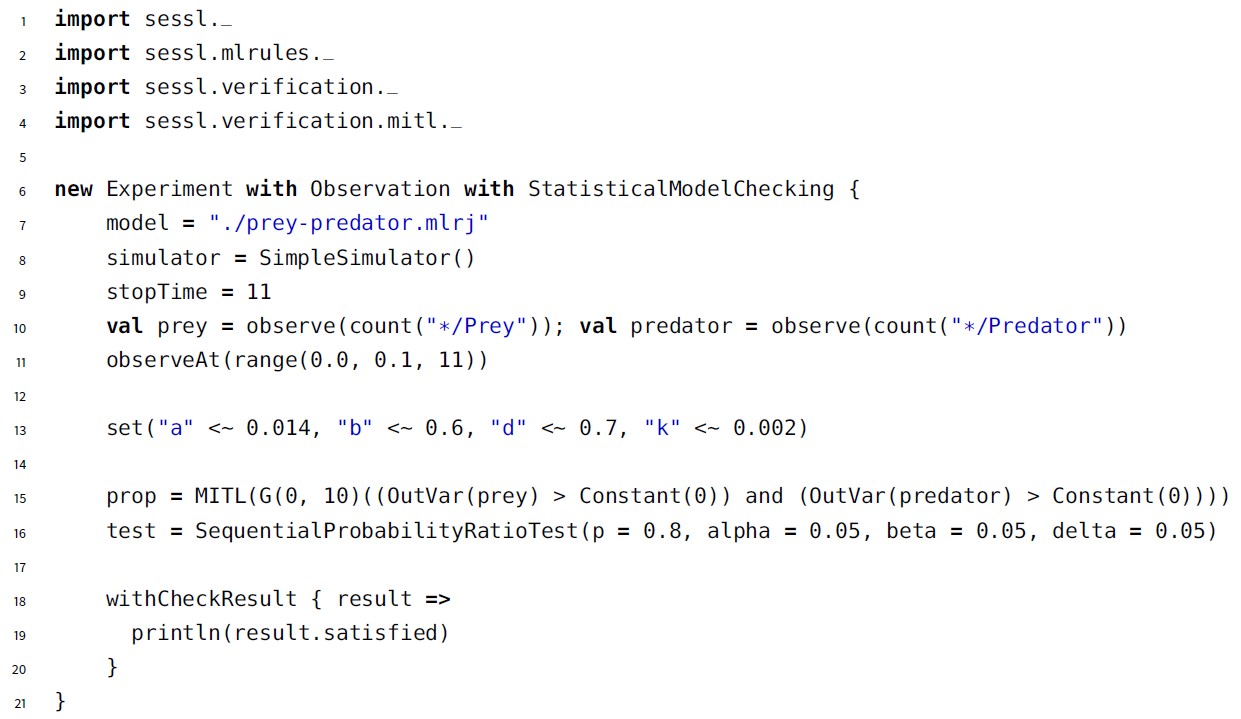
Figure 1 illustrates the working of SESSL with an example of statistical model-checking executed on a Lotka-Volterra ‘predator and prey’ model of interdependent dynamics of two populations, which has been defined in ML-Rules, a domain-specific modeling language for modeling and simulation in a different domain, namely systems biology (Maus et al. 2011). To perform a statistical model-checking experiment, the property to check must be explicitly defined. The experiment in Figure 1 checks for “coexisting state” (a commonly checked property of Lotka-Volterra models (Droz & Pękalski 2001) that states that both prey and predators will not become extinct (see Peng et al. 2014 for details).
Traits and bindings make the specification of simulation experiments in SESSL flexible and agile. Due to the automatic management of software artifacts, executing and repeating SESSL experiments is straightforward across machines and platforms. Based on SESSL, simulation experiments such as the statistical model checking shown above can even be automatically generated and executed to test whether specific behavior properties of models do still hold when models are extended (Peng et al. 2016) or composed (Peng et al. 2017). At the same time, SESSL specifications are succinct and readable, allowing easy sharing and communication of experiment specifications. This makes SESSL an excellent tool for experiment specification in domains that require diverse experiment design methods and non-standard approaches, such as agent-based computational demography.
ML3: A Modeling Language for Agent-Based Demographic Models
The Modeling Language for Linked Lives (ML3) (Warnke et al. 2015) is a domain specific modeling language specifically designed for agent-based demographic models with dynamic social networks. While most agent-based models are executed in a step-wise manner, and commonly used modeling environments such as Net-Logo (Wilensky 1999) pursue such a discrete-time approach, time in ML3 is continuous. This allows to capture the temporal behavior more realistically, and avoids many of the inherent problems of time-stepped simulation (Willekens 2009). The ML3 simulator software is implemented in Java (https://www.java.com) and distributed using Apache Maven. The ML3 Sandbox, an editor for ML3 models, is available for download in the ML3 repository (https://git.informatik.uni-rostock.de/mosi/ml3).
Key features of ML3
The primary entities of all ML3 models are agents, representing individual persons as well as higher-level demographic actors such as households. To distinguish the different kinds of entities that are modeled as agents, each agent has a type that determines its properties and behavior. Thus, each ML3 model begins with the definition of agent types. Figure 2 (lines 1 to 4) shows such an agent type definition. There, an agent type Person is defined. Every agent of this type has two attributes: their sex, which can have one of the two values "female" and "male", and their income, which is a real number. As aging of agents is an important part of many demographic models, e.g., with respect to fertility and mortality, all agents have an attribute age in addition to their explicitly defined attributes. During the simulation, the age of agents is initialized when an agent is "born", and updated automatically as time passes. Finally, all agents are either alive or dead. Agents are alive when they are created, and might die during the simulation. Dead agents do no longer act independently, but other agents might still be influenced by them.
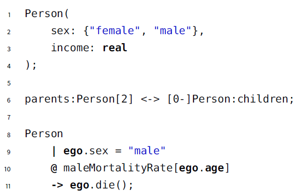
To facilitate the modeling of dynamically evolving social networks, these networks are an explicit part of an ML3 model. Agents in ML3 are interconnected with dynamic links, which model their relationships. For example, parents and their children might be connected with a link. The definition of the kinds of links agents of a certain type might have is the second part of every ML3 model, as Figure 2 (line 6) demonstrates for the example of parents and children. It reads as follows: Every person is linked to zero or more other persons, their children (read from left to right). Every person is also linked to exactly two other persons, their parents (read from right to left). Links are always directed (meaning the parent-direction is different from the children-direction), bi-directional (there has to be a parent-direction for the child-direction), and dynamic (links may change during the simulation, e.g., parents might get more children).
The behavior of agents is governed by stochastic rules. For each agent type, a set of behavioral rules must be defined, and those rules apply to all agents of that type that are currently alive. Rules are defined as guard-rate-effect triples, stating who is subject to the rule (guard), when the rule is applied (rate), and what happens when the rule is applied (effect). Figure 2 lines 8 to 11 shows a simple mortality rule as an example. The rule applies to all male persons (line 9). Its timing is governed by the rate expression (10). Here, the rate is given by the map maleMortalityRate, a special data structure ML3 uses to hold time-series data. In this case the map might hold the age-dependent force of mortality for different cohorts as it might have been estimated from data. The rate expression gives the (possibly time dependent) parameter of an exponential distribution. Finally, the rule ends with the effect (line 11). In the case of this mortality rule, the agent simply dies. During the simulation for each pair of agent and rule a waiting time is drawn from the according waiting time distribution, and the agent-rule pair with minimal waiting time is executed. In addition to stochastically timed rules, which are the most commonly used, ML3 supports a range of deterministic ways to schedule an event, e.g., to schedule events when an agent reaches a certain age or to schedule periodic events.

StatisticalModelChecking trait that lives in the SESSL verification package. The process is repeated until enough simulation runs have been observed to decide whether the property is satisfied or not.The SESSL-ML3 Binding
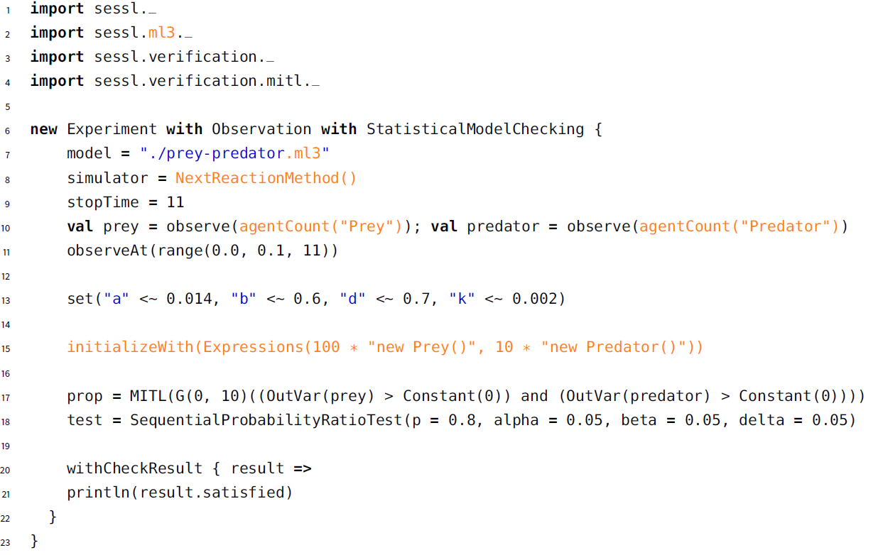
To exploit the features of SESSL for experimentation with ML3 models, we implemented a SESSL binding for ML3. The binding covers the basic features of SESSL experiments, such as choosing a model file and a simulation algorithm, setting simulation stop conditions and replication numbers, configuring parallel execution, and the observations made during the simulation. Similar as in other SESSL bindings for simulation packages, all specifications are translated to API (application programming interface; the interface through which other software communicates with a piece of software) calls of the ML3 package. A sketch of the call hierarchy of an experiment is shown in Figure 3. In Figure 4, an experiment identical to the one shown in Figure 1 is specified using SESSL-ML3 instead of ML-Rules.
In addition to traits for the generic experiment aspects, we also implemented experiment aspects in the binding that are specific to ML3. To realize the binding for ML3 we adopted a new concept of model parameterization. Previous SESSL bindings executed models with scalar model inputs. However, as ML3 models are aimed at describing demographic phenomena, many model parameters are time series data or distributions, which ML3 represents as parameter maps. For example, for individuals the risk of dying depends on their age (see Figure 2 line 10). The pattern of age-dependent event rates is typical for applications in demography. In the return migration model the age distribution at migration is realized as a parameter map. Consequently, we implemented a trait ParameterMaps that allows reading in parameter maps from .csv files. The software implementation is available on-line in the official SESSL repository (sessl.org) under an open-source license.
Illustration: A Model of Return Migration
As a first case study, we present a novel but prototypical and relatively simple agent-based model of return migration. To illustrate the main features of our experimental approach in a succinct and transparent way, we use this simple model rather than a more complex one, which is discussed next. Primarily the model consists of four processes: the inflow of migrants into the system; the formation of a social network between the migrants; the employment and earnings of the migrants, depending on the social network; and the decision of migrants to return to their country of origin. The model is kept simple on purpose, to capture only the main features of the migration processes of interest, enabling to illustrate the process of the experimental design with a flexible simulation environment offered by ML3 and SESSL. Following the approach of Cioffi-Revilla (Cioffi-Revilla 2010) the model, as presented here, is merely a relatively simple initial model version \(M_0\). The results of the experiments we conduct with this initial model suggest a way forward for refinement of the model in an iterative process, by which through identifying the model parameters of key importance, and possibly collecting additional information allowing for identifying them better, we would be able to design subsequent model versions (Courgeau et al. 2016). For more realistic applications, a comprehensive review of recent advancements in agent-based modeling of migration is provided by (Klabunde & Willekens 2016).
The primary entities of our models are migrant agents. Migrants are characterized by a number of attributes that influence their economic success and their behavior regarding their return migration decision (Figure 5). Migration streams predominantly consist of younger migrants, and so the simulated ages of new migrants are drawn from a distribution reflecting this. The distribution was constructed by fitting a 5-parameter model based on that developed by Rogers (1978) to UK migration data from the Office of National Statistics; it is provided to the simulation as an input file. Migrant age is significant in the model as once a predetermined retirement age is reached (60 for the runs described here), agents are removed from the simulation. In a later model version other processes, e.g., employment and income, might also depend on age.
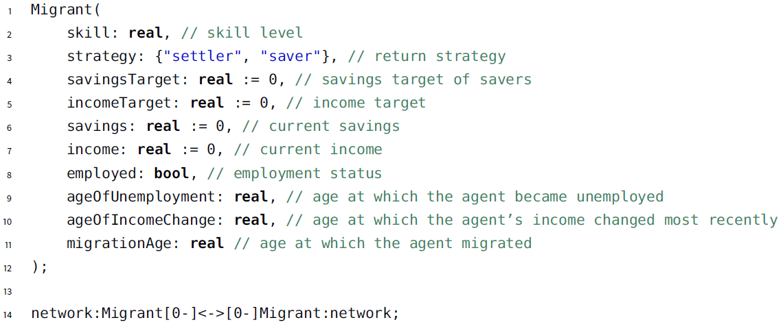
Simulated migrants are also endowed with a randomly determined ’skill level’ which determines their earnings potential. This reflects migrants differing ability to succeed in the host country, which is often incorporated into similar economic models (Borjas & Bratsberg 1996; Dustmann et al. 2011). Skill levels are drawn from a normal distribution centered on 1 and truncated from below at 0. The variance of this distribution is a variable parameter in the model. As well as possessing these characteristics, the migrants are also part of a social network (Figure 5, line 14). Each migrant is linked to a number of other migrants, and refers to them as their network. These network links are bidirectional, so if A is part of B’s network, B is also part of A’s network. The complete social network forms an undirected graph.
On initialization, there are no migrants present in the system. Migrants enter the system stochastically with exponentially distributed inter-arrival times. The rate depends upon the difference between the current average earnings and migrant’s target earnings, in line with economic theory, which suggests, that migrant flow de-pends on earnings differentials (Harris & Todaro 1970). In the ML3 implementation this process is governed by a stochastic rule (Figure 6). When the rule is executed, a new migrant agent is created (line 4) and its attributes are initialized according to the respective distributions (lines 5-10 and 19-25), and the new migrant is introduced into the network (lines 12-18).
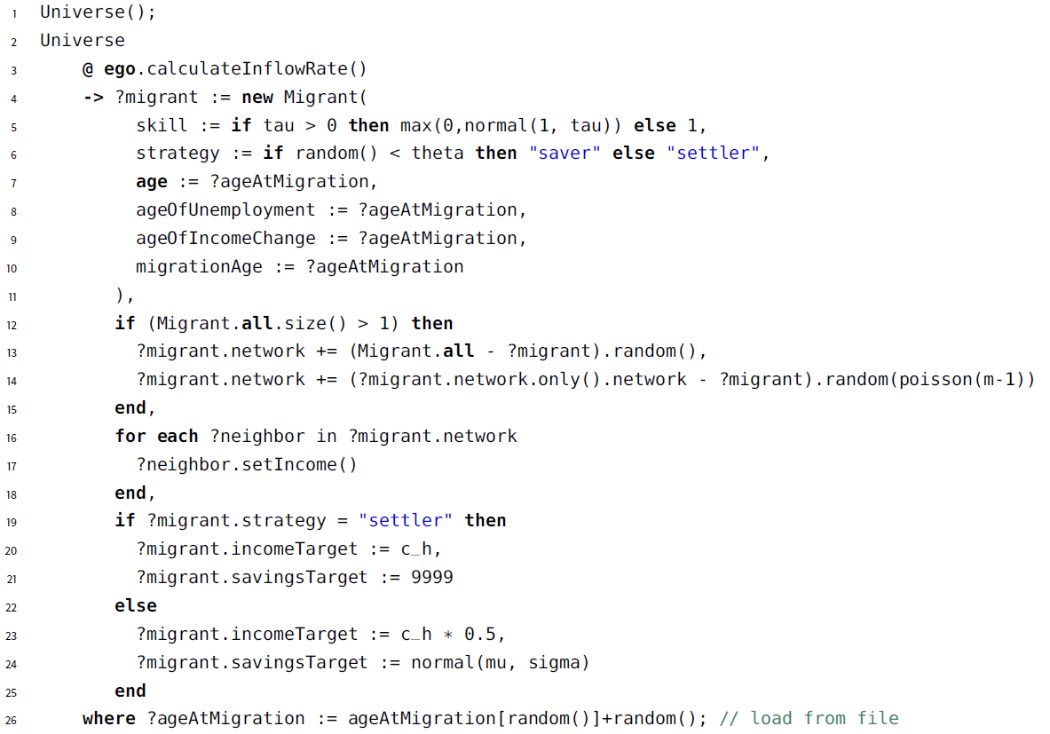
Network ties are determined on entry to the system, with an initial ‘contact’ chosen at random for each new migrant from those agents already in the system, and further ties made from amongst this contact’s neighbors. This reflect the tendency for migrants’ moves to be facilitated by someone they already know in the host country (Liu 2013). When an agent leaves the system (either because they have satisfied one of the return migration conditions described below, or they have reached the retirement age), their network ties are removed.
Migrants also participate in labor markets after migration. The model of the labor market used is relatively crude. Employment opportunities come along at a fixed rate (although the model allows for unemployment to increase as more migrants enter the system). Wages are assumed to respond to labor supply, so that more mi-grants in the system results in lower wages. More specifically, labor unit prices respond quadratically to supply. Of course, the precise relationship between migrant wages and number of immigrants depends on the many factors including local labor market conditions and production technology; however, for an initial choice, diminishing returns from labor would appear to be an appropriate assumption, and similar assumptions have been made elsewhere (Epstein 2008). However, skill-based heterogeneity in earnings amongst migrants is included as a multiplier to this basic relationship as shown in Equation 1. Future models could include explicit price setting and bargaining based upon the information and preferences of both employer(s) and migrants.
| $$y_i = s_i ( \alpha - \beta N^{2})$$ | (1) |
Total income or utility is affected not only by earned income but also through social capital associated with the extent of a migrant’s network. In line with work by Portes (1998), the social capital associated with migrant networks could realize itself in a number of forms, including access to credit and housing, sharing of information regarding the host country, loaning of durable goods, or provision of childcare. Although these are generally provided in non-monetary forms, it is presumed here that they act to increase net income by reducing expenditure on certain goods; the benefit it provides is fungible (ibid). In empirical work, it is often assumed that the relevant quantity determining network effects is the total number of migrants present in a given location (Epstein 2008, e.g.). However, in this case, the specific number of network ties each migrant has determines their social capital. It is assumed that there are diminishing returns to migrant social capital so that the amount of social capital provided by network ties decreases as the number of ties increases, as shown in Equation 2. The sum of Equations 1 and 2 defines the total income of the migrant.
| $$k = \gamma log(1 + g)$$ | (2) |
Agents are presumed to follow one of two strategies: either they intend to settle permanently in their new country of residence; or they wish to save until they reach some target value which will allow them to live more comfortable in their country of origin. This distinction between temporary and permanent migrants in incoming migration streams has support in empirical migration literature (Constant & Massey 2002; Bijwaard 2007, e.g). These strategies define the rules used to describe when agents migrate back to their home country.
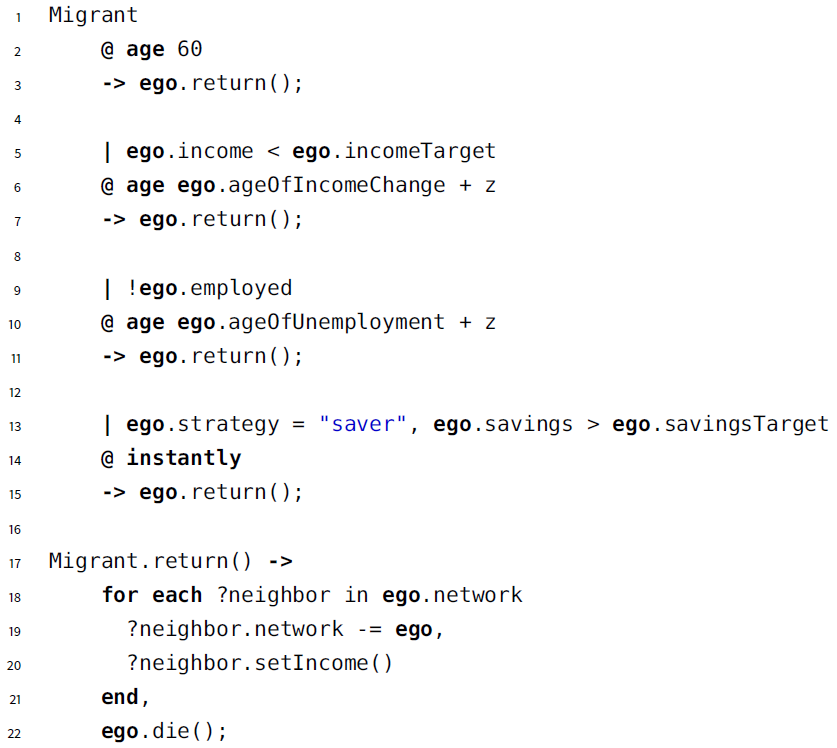
In the case of permanent ‘settler’ migrants, migrants return if they earn less than some minimum value \(C\) (Figure 7, line 5). Their counterparts, ‘saving’ migrants, instead return once they reach some target value \(T\) (Figure 7, line 13), which is drawn from a normal distribution (although an income target for ‘savers’ is also defined, but at a lower value, as they are willing to accept lower current consumption in favor of later reward upon return to their country of origin). If the minimum income conditions are met, migrants do not leave immediately; instead, they remain in the country for a short period \(z\) in case the situation changes, before finally returning.
The relative frequency of ‘savers’ in the immigrant distribution is determined by parameter \(\theta\). Different proportions of the two migrant types may be expected to produce different behavior in the overall system, both because of their individual characteristics and due to potential emergent properties resulting from their interdependence in the network. However, in order to assess the relative influence of the different elements of the model on the proportion of ‘savers’, a more thorough and systematic experimentation is required.
Experiments with the Migration Model
Thanks to the binding between SESSL and ML3, all features of SESSL are now ready to use for agent-based models specified in ML3, including the migration model presented in the previous section. The variety of experiment designs, of optimization methods and statistical model checking, form an expressive portfolio for analyzing the behavior of agent-based models in demography. However, so far one class of experimental methods has not been supported: meta-modeling, which increasingly receives attention, also in the area of agent-based demography (Bijak et al. 2013; Silverman et al. 2013a). Meta-models, or response surfaces, or surrogate models, pro-vide means to approximate the input-output function that is realized by the underlying simulation model. They are in fact statistical models of the underlying simulation models. As such, they are used in many application fields (see, for example, the Managing Uncertainty in Complex Models project, http://www.mucm.ac.uk). The meta-models are particularly useful, whenever the calculation of individual simulation runs, and thus parameter scans or optimizations, imply significant computational effort and expense.
To demonstrate how SESSL can be extended to this new class of analytical methods for agent-based models, two examples of meta-models are derived based on two experimental designs. Firstly, a regression-based meta-model is fit to a parameter scan relying on central composite design (Kleijnen 2008), and secondly, a Gaussian Process emulator is used to analyze a Latin hypercube sample obtained in a second set of experiments (Kennedy & O’Hagan 2001). In both cases, the links between the different designs and analysis models are natural, as central composite designs assume relationships between variables which can be captured through the low-order polynomials used in regression meta-models. In contrast, Gaussian processes are semi-parametric, meaning that no particular functional form for the relationship between inputs and outputs is assumed, and thus the more flexible Latin hypercube design is preferable. More complex stochastic models might even ask for additional methods to deal with the high-dimensionality of agent-based models effectively, e.g., (Salemi et al. 2016).
With the two meta-models we employ two different strategies for SESSL to be integrated into an experimentation workflow. For the linear regression meta-model, the whole process of fitting the meta-model is part of the experiment specified in SESSL. This includes the execution of the central composite design as well as the actual fitting of the regression model. However, for the Gaussian process meta-model we demonstrate a different approach. While SESSL is used to conduct the simulation runs according to the Latin Hypercube design, the meta-model is fitted with an external tool. To this end, the SESSL experiment produces CSV files containing the data produced by the simulation. Those can then be processed externally, in our case using the R statistical programming language (R Development Core Team 2017). This approach has the advantage of added flexibility, as the simulationist is not restricted to the methods provided by SESSL itself. However, the advantages SESSL offers for documentation and reproducibility are partly lost. While the documentation and reproducibility is still ensured by SESSL for the experimental setup, it is not for the fitting of the regression model.
Example 1: Central Composite Design and Regression Meta-models
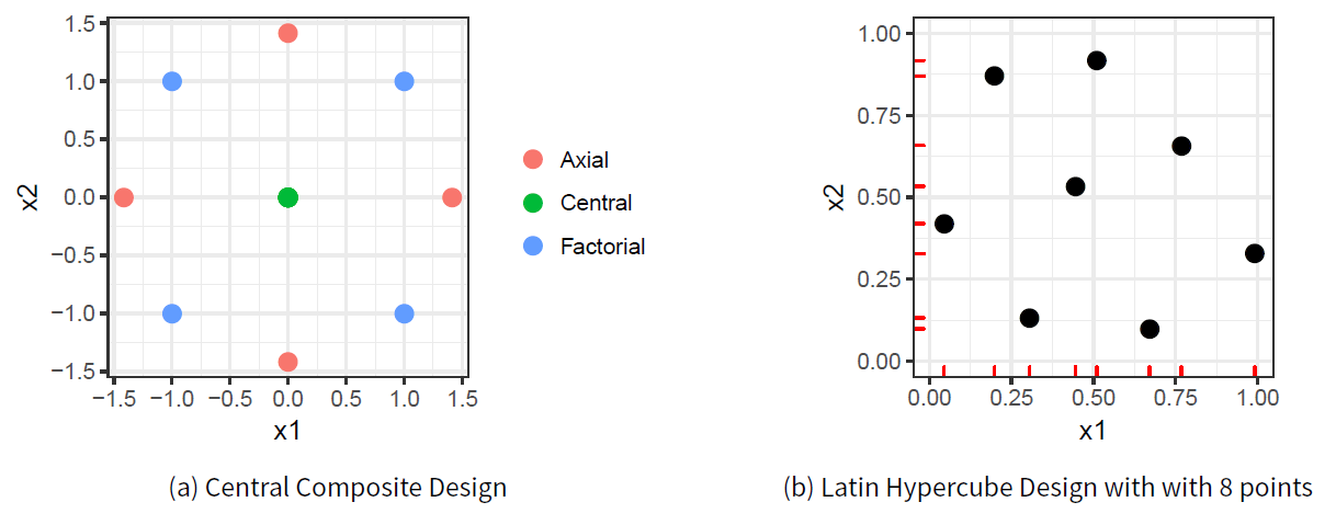
Experimental design allows to gain information about the relationships between experimental inputs and outputs by controlling the location of input points. A central composite design provides for the identification of second-order polynomial relationships in the data. It consists of the combination of three sets of points (factorial, axial and central), as detailed in Figure 8 (a). The first such set is generally a two-level factorial (grid-based) design, where each parameter is assigned a high and low value, and all combinations of these parameter values are identified. Secondly, a set of axial points are identified, whereby all parameters but one are set to their central value, and the remaining parameter is given extreme values (beyond those used for the factorial design). Finally, a central point is defined, where all parameters are set to their central value. Generally, repeated runs are used at the central point to gain information about the inherent stochasticity of the system under study (in the case of stochastic simulation, this is the part of variability in output caused by pseudo-random number generation, and unrelated to parametric changes). Although Figure 8 displays only two dimensions, the design generalizes naturally to higher dimensions.
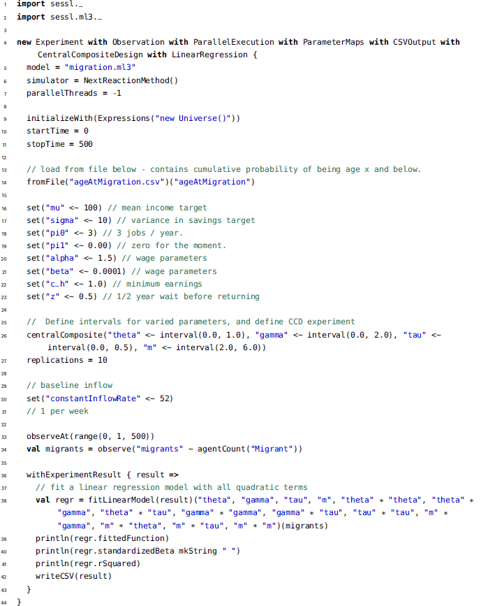
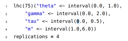
Parameters controlling the degree of heterogeneity in ‘skill’ \(\tau\); the proportion of savers and settlers in the population \(\theta\); the number of initial network ties \(m\) and the extent to which network ties effect overall earnings \(\gamma\) were varied for this case study. Initially, the aim was to understand the effect of these parameters on the steady-state number of total migrants in the system. Although time is continuous in the ML3 simulations, avoiding problems of simultaneity, in this case counts of migrants were observed every year for ease of interpretation. Figure 9 provides the SESSL code needed to define the experiment described, with the design itself specified at line 26, and the regression meta-model at line 38.
The estimates of standardized coefficients are given in Figure 10. Considering the main (linear) effects, it can be seen that \(\theta\) and \(\gamma\) have the largest effects on the average number of migrants in the system. The quadratic and interaction effects underline the importance of these variables, while the heterogeneity in skill \(\tau\) and number of network ties \(m\) appear to have little effect.

Example 2: Latin Hypercube Sample and Gaussian Process Emulator
A similar experiment was defined varying the same parameters and monitoring the same output variable, but utilizing a different design and meta-model; a Latin hypercube design was used to fit a Gaussian Process emulator to the data. A Latin hypercube sample is a space-filling design which divides each dimension into regularly sized bins equal to the number of desired observations, and chooses points pseudo-randomly in such a way that there is exactly one observation in each bin for every dimension. In contrast to a factorial or grid-based design, it does not repeat values of any single parameter (Urban & Fricker 2010), as can be seen from the tick marks along the axis in Figure 8. As with the Central Composite design, the Latin Hypercube design generalizes easily to higher dimensions and can be specified in SESSL with a simple command, as shown in Figure 11 (b).
Gaussian process emulators work on the assumption that values close to each other in input space will also be close to each other in terms of output. More specifically, outputs are considered to be jointly multivariate normal, with the degree of correlation determined by a covariance function operating on inputs. Full details can be found in Kennedy & O’Hagan (2001). Gaussian process are flexible in that they don’t make assumptions about the possible shapes of the output as a function of inputs, with the exception that some degree of smoothness is assumed, to be estimated from the data.
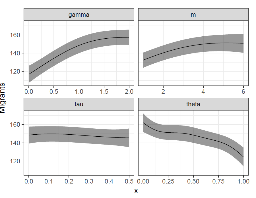
Once fitted, the emulator can be used to produce predictive probability distributions for output values at any combination of input points, incorporating both the uncertainty about the mean value of the simulation at that point, and uncertainty about the degree of underlying simulation stochasticity (Kennedy & O’Hagan 2001). In this example, we have used the implementation of the method presented in Hilton & Bijak (2016). Predictions at mean values across the range of each covariate are displayed in Figure 12. The results are broadly consistent with the results obtained from the meta-model, although local movements in the mean surface are captured, as can be seen to some extent in the predictions over the range of the settler-saver-proportion \(\theta\) in the Figure.
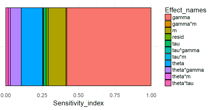
A more comprehensive view can be gained by conducting a global sensitivity analysis of our initial model \(M_0\); this examines the proportion of the total variance that can be attributed to each variable and combination of variables, averaged over prior distribution on these variables. The mathematical details can be found in Kennedy & O’Hagan (2001), and a summary in Silverman et al. (2013a). In our example, as can be seen from the Figure 13, in model \(M_0\) the majority of the variance is associated with \(\theta\) and \(\gamma\), in agreement with results from the meta-model coefficients displayed in Figure 10, although a significant part is also related to \(m\).
These results indicate that the next phase of the model-building process should concentrate on obtaining more information about \(\theta\) and \(\gamma\), rather than focus on \(\tau\) or \(m\). This can be possibly achieved by conducting a survey-based or experimental empirical study pertaining to these parameters, including the propensity for saving (\(\theta\)) and reactivity to the network size (\(\gamma\)), in order to produce the next, more refined version of the model, \(M_1\), and so on. The philosophical justification and a general outline of this iterative approach is given in Courgeau et al. (2016).
A Model of Social Care
To demonstrate that our approach is also applicable to larger scale models, we executed a further simulation experiment on a linked lives model of social care by Noble et al. (2012), that aims at capturing the effects of the aging population and changing family structures on the cost of state-funded social care in the United Kingdom (UK). The model is concerned with the demographic processes that affect the supply and demand of social care. In the model, the population of the UK is represented by agents with a scaling factor of \(1:10,000\), i.e. one agent represents \(10,000\) people in the real world. For all agents life-course transitions that are important for social care, e.g., fertility, mortality, partnership formation and internal migration, are simulated. Agents are born as dependent children of their parents. With age 17, they reach adulthood. At this point they enter the workforce and become a taxpayer. They may marry another agent, move to a different part of the UK, and get children of their own. When they reach the retirement age, they retire and leave the workforce. Anytime during their life, their health status might degrade, which increases their need for social care. Finally, they die, which removes them from the population. For the purpose of internal migration, the model divides the UK into a grid of towns, with consist of multiple houses. Agents may migrate to a different house in the same town or to a different town multiple times in their life. We have reimplemented the model, originally implemented in Python, in ML3 (Warnke et al. 2015).
The central output variable of the model is the total cost of social care per taxpayer. Every agent needs a certain amount of social care, measured in hours per week, depending on their care need category – which may include zero. A part of this care need can be fulfilled informally by relatives, the rest needs to be paid for by the state. Individuals who need no or only little care themselves can provide some hours for informal care each week. However, they will not deliver care to anybody, but only to persons living in the same household and to their parents, as long as the parents live in the same town. The care they can deliver is distributed among the persons they are willing to care for. Therefore, household structures and mobility affect the amount of informal social care that is actually delivered.
Given the high complexity of this model, in this section we present only the key high-level features and findings related to the conducted experiments. In particular, we show a simulation-based optimization experiment, a further experimental method supported by SESSL. The term simulation-based optimization refers to the search for those values of model input parameters that minimize or maximize an objective, which is a function of the simulation output (Amaran et al. 2017). Simulation-based optimization is commonly employed for model calibration, by minimizing the difference between the simulated model output and the calibration target. While meta-models can also be used for optimization purposes (Barton & Meckesheimer 2006) they cannot yield satisfying results for all optimization problems, e.g., with discontinuous objective functions, many input variables or discrete inputs (Nguyen et al. 2014). There is no ’one-size-fits-all’ optimization method, and a plethora of algorithms exist for different classes of optimization problems (see Amaran et al. 2017 for an overview). In SESSL simulation-based optimization is realized through a binding to the Opt4J (Lukasiewycz et al. 2011) library of optimization algorithms, allowing the user to choose between many different methods.
In the experiment (Figure 14), we want to minimize the cost of social care per taxpayer by varying the retirement age. Therefore, we embedded the experiment specification (line 2–43) in a minimize-block, which is provided by the SESSL-Opt4J binding. As the calculation of the cost of social care is very complex (see Section 6.2), it cannot be realized with SESSL-ML3. However, we can exploit the extendibility of SESSL, by implementing a custom observation directly using the observation-interface of the ML3 simulator. We have wrapped that in the trait HealthCareCostObservation (lines 2 and 35). Similarly, we have implemented a custom initial state builder (line 5), which creates the initial state exactly as in the Python implementation of the model. In both cases, SESSL allows for making direct calls to the more powerful, but difficult to use, API of the ML3 simulator when necessary, while keeping the easy to use features of SESSL when possible.
In line 31 the model parameter for the age of retirement is set to the value chosen by the optimization algorithm. In lines 38–43 the objective function of the optimization is calculated. The optimization itself is then parameterized after the experiment specification, where a range for the retirement age parameter and an optimization algorithm are chosen. The optimization yields a minimum of the cost of social care by setting the retirement age to about 73, with a weekly cost per taxpayer of £74.95. This is in line with the findings of Silverman et al. (2013b) that care cost per taxpayer actually increases when the retirement age is increased beyond 70, as the increased number of taxpayers will be o set by the reduction of available informal care in households with elderly members.
To apply an experimental method in practice, the computational effort needs to be reasonably low. In the above experiment, as single run is executed in about 6.3 minutes on a powerful desktop machine (Intel Core i7 990X at 3.46 GHz). For the whole experiment, consisting of 500 runs (10 iterations of the optimization algorithm with 5 particles and 10 replications each), exploiting parallel execution of replications, this yields a runtime of about 12.5 hours. For large-scale simulation models the majority of the computational effort of complex simulation experiments such as statistical model checking, meta-modeling, and simulation-based optimization lies in execution of the single simulation runs. However, for computationally very intensive models, the approach using SESSL allows for minimizing the number of simulation runs, e.g., by employing advanced experimental designs, such as the Latin Hypercube and central composite designs shown before, which need only few design points to give meaningful results.
Discussion
The review about benefits and limitations of the ODD protocol (Overview, Design concepts, and Details), which was published in 2006 to standardize the description of agent-based models (Grimm et al. 2010), recommends to enhance ODD by a separate section on simulation experiments. Information about experiments done with a model supports assessing the range for which a model might be valid, interpreting and questioning published simulation results, which is essential in valuing and reusing models. In addition, compact, declarative specifications of simulation experiments facilitate the generation and adaptation of simulation experiments in general, and with agent-based models in particular. They contribute to a more efficient and systematic engineering of simulation experiments (Teran-Somohano et al. 2015).
SESSL (Simulation Experiment Specification via a Scala Layer) is a domain-specific language for supporting the specification and execution of simulation experiments. It presents a simulation-system-agnostic layer between simulation system and user and supports a wide variety of simulation experiments, including specific experiment designs, parameter scans, simulation-based optimization, and statistical model checking. Due to the new presented binding between SESSL and ML3 (Modeling Language for Linked Lives), the entire methodological portfolio provided in SESSL can now be used for experimenting with agent-based models specified in ML3 and for documenting these simulation experiments in a non-ambiguous manner.
As an internal domain specific language, SESSL facilitates adaptations and extensions for particular application domains. For demographic models, we realized and integrated a new experimental design method, i.e., central composite design, and two meta-modeling methods, i.e., regression meta-models and a Gaussian process emulator. We combined them with further methods SESSL already supported to analyze a simple agent-based return migration model and a more complex model of social care. The resulting simulation experiments can be succinctly described, executed, and adapted in SESSL and show that in this model the parameters for migrant strategies distribution and network ties are crucial for the system’s behavior. The binding between SESSL and ML3 demonstrates the potential of domain specific languages for conducting and documenting simulation experiments with agent-based models in a convenient, replicable, and at the same time, flexible manner.
Following the suggestions by Courgeau et al. (2016), Gray et al. (2017) and Burch (2018), these developments can substantially enhance the explanatory power of agent-based models, especially in such a strongly empirical discipline as demography. On the one hand, they can help connect the micro and macro levels of analysis Billari (2015), and provide a template for designing theoretical microfoundations explaining population-level phenomena in a rigorous and systematic way. At the same time, the proposed approach remains within the spirit of the Manifesto of Computational Social Science (Conte et al. 2012), arguing for a greater empirical relevance of social simulation models, for example with respect to modelling the human decision processes involved (Klabunde et al. 2017), and also helping unravel the mechanisms underpinning the social processes under study. The approach proposed in this paper provides a blueprint – as well as efficient software tools – for addressing these research challenges in a systematic fashion through an iterative process of design, execution, analysis and documentation of computer experiments. Further developments in this area could include integrating a full statistical analysis, which would additionally enable the estimation of the free model parameters given the available data and assessing the uncertainty of the variables of interest. The ultimate goal of this process is to enhance the analytical possibilities offered by social simulations by embedding them within the wider framework of experimental design – and by bringing in this way the empirical and theoretical aspects of demographic enquiries closer together.
Acknowledgements
This research is supported by the German Research Foundation (DFG) via research grant UH-66/15-1; by the Economic and Social Research Council (ESRC) Centre for Population Change | phase II, grant ES/K007394/1, and by the European Research Council (ERC), via grant CoG-2016-725232 Bayesian Agent-Based Population Studies.References
AGHA, G. & Palmskog, K. (2018). A survey of statistical model checking. ACM Transactions of Modeling and Computer Simulation – TOMACS, 28(1), 6. [doi:10.1145/3158668]
AMARAN, S., Sahinidis, N. V., Sharda, B. & Bury, S. J. (2017). Simulation optimization: A review of algorithms and applications. Annals of Operations Research, 240(1), 351–380.
APARICIO Diaz, B., Fent, T., Prskawetz, A. & Bernardi, L. (2011). Transition to parenthood: the role of social interaction and endogenous networks. Demography, 48(2), 559–79. [doi:10.1007/s13524-011-0023-6]
BARTON, R. R. & Meckesheimer, M. (2006). Chapter 18 Metamodel-Based Simulation Optimization. In S. G. Hender-son & B. L. Nelson (Eds.), Handbooks in Operations Research and Management Science, vol. 13, (pp. 535–574). Amsterdam: Elsevier.
BIJAK, J., Hilton, J., Silverman, E. & Cao, V. D. (2013). Reforging the wedding ring: Exploring a semi-artificial model of population for the United Kingdom with Gaussian process emulators. Demographic Research, 29(27), 729– 766. [doi:10.4054/DemRes.2013.29.27]
BIJWAARD, G. E. (2007). Modeling Migration Dynamics of Immigrants: The Case of The Netherlands, Institute for the Study of Labour / Forschungsinstitut zur Zukuft der Arbeit, IZA Discussion Paper 2891: https://papers.ssrn.com/sol3/papers.cfm?abstract_id=1000139.
BILLARI, F., Fent, T., Prskawetz, A. & Aparicio Diaz, B. (2007). The "Wedding-Ring": An Agent-Based Marriage Model Based on Social Interactions. Demographic Research, 17, 59–82. [doi:10.4054/DemRes.2007.17.3]
BILLARI, F. & Prskawetz, A. (Eds.) (2003). Agent-Based Computational Demography. Using Simulation to Improve Our Understanding of Demographic Behaviour. Heidelberg: Springer.
BILLARI, F. C. (2015). Integrating macro- and micro-level approaches in the explanation of population change. Population Studies, 69(Suppl.), S11–S20. [doi:10.1080/00324728.2015.1009712]
BORJAS, G. & Bratsberg, B. (1996). Who leaves? The outmigration of the foreign-born. Review of Economics and Statistics, 78(1), 165–176.
BURCH, T. K. (2018). Model-Based Demography. Essays on Integrating Data, Technique and Theory. Cham: Springer. [doi:10.1007/978-3-319-65433-1]
CIOFFI-REVILLA, C. (2010). A methodology for complex social simulations. Journal of Artificial Societies and Social Simulation, 13(1), 7: https://www.jasss.org/13/1/7.html. [doi:10.18564/jasss.1528]
COALE, A. (1973). The demographic transition reconsidered. In Proceedings of the International Population Conference, (pp. 53–72). Liege: Ordina Editions.
CONSTANT, A. & Massey, D. S. (2002). Return Migration by German Guestworkers: Neoclassical versus New Economic Theories. International Migration, 40(4), 5–38.
CONTE, R., Gilbert, N., Bonelli, G., Cioffi-Revilla, C., Deffuant, G., Kertesz, J., Loreto, V., Moat, S., Nadal, J. P., Sanchez, A., Nowak, A., Flache, A., San Miguel, M. & Helbing, D. (2012). Manifesto of computational social science. The European Physical Journal Special Topics, 214(1), 325–346. [doi:10.1140/epjst/e2012-01697-8]
COURGEAU, D., Bijak, J., Franck, R. & Silverman, E. (2016). Model-based demography: Towards a research agenda. In J. van Bavel & A. Grow (Eds.), Agent-Based Modelling in Population Studies: Concepts, Methods, and Applications, (pp. 29–51). Dordrecht: Springer.
DROZ, M. & Pękalski, A. (2001). Different strategies of evolution in a predator-prey system. Physica A: Statistical Mechanics and its Applications, 298, 545–552. [doi:10.1016/S0378-4371(01)00271-0]
DUSTMANN, C., Fadlon, I. & Weiss, Y. (2011). Return migration, human capital accumulation and the brain drain. Journal of Development Economics, 95(1), 58–67.
EPSTEIN, G. S. (2008). Herd and Network Effects in Migration Decision-Making. Journal of Ethnic and Migration Studies, 34(4), 567–583. [doi:10.1080/13691830801961597]
EWALD, R. & Uhrmacher, A. M. (2014). SESSL: A domain-specific language for simulation experiments. ACM Transactions on Modeling and Computer Simulation, 24(2).
FENT, T., Aparicio Diaz, B. & Prskawetz, A. (2013). Family policies in the context of low fertility and social structure. Demographic Research, 29, 963–998. [doi:10.4054/DemRes.2013.29.37]
GRAY, J., Hilton, J. & Bijak, J. (2017). Choosing the choice: Reflections on modelling decisions and behaviour in demographic agent-based models. Population Studies, 71(Supp.), 85–97.
GRAZZINI, J. & Richiardi, M. G. (2013). Consistent Estimation of Agent-Based Models by Simulated Minimum Distance. Tech. Rep. 130, Laboratorio Riccardo Revelli.
GRIMM, V., Berger, U., DeAngelis, D. L., Polhill, J. G., Giske, J. & Railsback, S. F. (2010). The {ODD} protocol: A review and first update. Ecological Modelling, 221(23), 2760–2768.
GROW, A. & Van Bavel, J. (2015). Assortative Mating and the Reversal of Gender Inequality in Education in Europe: An Agent-Based Model. PLoS ONE, 10(6): e0127806. [doi:10.1371/journal.pone.0127806]
HARRIS, J. R. & Todaro, M. P. (1970). Migration, Unemployment and Development: a Two-Sector Analysis. American Economic Review, 60(1), 126–142.
HEDSTRÖM, P. & Ylikoski, P. (2010). Causal mechanisms in the social sciences. Annual Review of Sociology, 36, 49–67. [doi:10.1146/annurev.soc.012809.102632]
HILLS, T. & Todd, P. (2008). Population Heterogeneity and Individual Differences in an Assortative Agent-Based Marriage and Divorce Model (MADAM) Using Search with Relaxing Expectations. Journal of Artificial Societies and Social Simulation, 11(4), 5: https://www.jasss.org/11/4/5.html.
HILTON, J. & Bijak, J. (2016). Design and analysis of demographic simulations. In J. van Bavel & A. Grow (Eds.), Agent-Based Modelling in Population Studies: Concepts, Methods, and Applications, (pp. 301–340). Dordrecht: Springer.
HOBCRAFT, J. (2007). Towards a scientific understanding of demographic behaviour. Population – English Edition, 62(1), 47–51.
KAMIŃSKI, B. (2015). Interval metamodels for the analysis of simulation Input-Output relations. Simulation Modelling Practice and Theory,54, 86–100. [doi:10.1016/j.simpat.2015.03.008]
KASHYAP, R. & Villavicencio, F. (2016). The Dynamics of Son Preference, Technology Diffusion, and Fertility Decline Underlying Distorted Sex Ratios at Birth: A Simulation Approach. Demography, 53, 1261–1281.
KENNEDY, M. & O’Hagan, T. (2001). Bayesian calibration of computer models. Journal of the Royal Statistical Society, Series B, 63(3), 425–464. [doi:10.1111/1467-9868.00294]
KLABUNDE, A. (2014). Computational Economic Modeling of Migration. Tech. Rep. 471, Ruhr University Bochum, Bochum.
KLABUNDE, A. & Willekens, F. (2016). Decision-making in agent-based models of migration: State of the art and challenges. European Journal of Population, 32(1), 73–97. [doi:10.1007/s10680-015-9362-0]
KLABUNDE, A., Zinn, S., Willekens, F. & Leuchter, M. (2017). Multistate modelling extended by behavioural rules: An application to migration. Population Studies, 71(Supp.), 51–67.
KLEIJNEN, J. P. (2008). Design and Analysis of Simulation Experiments. New York, NY: Springer.
LIU, M.-M. (2013). Migrant networks and international migration: testing weak ties. Demography, 50(4), 1243–77.
LORIG, F., Becker, C. & Timm, I. (2017). Formal specification of hypotheses for assisting computer simulation studies. In Proceedings of the 2017 SpringSim TMS-DEVS Conference, SpringSim’17. SCS Press.
LUKASIEWYCZ, M., Glaß, M., Reimann, F. & Teich, J. (2011). Opt4J - A Modular Framework for Meta-heuristic Opti-mization. In Proceedings of the Genetic and Evolutionary Computing Conference (GECCO 2011), (pp. 1723–1730). Dublin, Ireland.
MALER, O. & Nickovic, D. (2004). Monitoring Temporal Properties of Continuous Signals. In Formal Techniques, Modelling and Analysis of Timed and Fault-Tolerant Systems, Lecture Notes in Computer Science, (pp. 152–166). Berlin, Heidelberg: Springer. [doi:10.1007/978-3-540-30206-3_12]
MAUS, C., Rybacki, S. & Uhrmacher, A. M. (2011). Rule-based multi-level modeling of cell biological systems. BMC Systems Biology, 5(166).
MCKAY, M. D., Beckman, R. J. & Conover, W. J. (2000). A comparison of three methods for selecting values of input variables in the analysis of output from a computer code. Technometrics, 42(1), 55–61. [doi:10.1080/00401706.2000.10485979]
NGUYEN, A.-T., Reiter, S. & Rigo, P. (2014). A review on simulation-based optimization methods applied to building performance analysis. Applied Energy, 113, 1043–1058.
NOBLE, J., Silverman, E., Bijak, J., Rossiter, S., Evandrou, M., Bullock, S., Vlachantoni, A. & Falkingham, J. (2012). Linked Lives: The Utility of an Agent-based Approach to Modeling Partnership and Household Formation in the Context of Social Care. In Proceedings of the WSC 2012, (pp. 93:1–93:12). [doi:10.1109/WSC.2012.6465264]
PENG, D., Ewald, R. & Uhrmacher, A. M. (2014). Towards semantic model composition via experiments. In Proceedings of the 2Nd ACM SIGSIM Conference on Principles of Advanced Discrete Simulation, SIGSIM PADS ’14, (pp. 151–162). New York, NY, USA: ACM.
PENG, D., Warnke, T., Haack, F. & Uhrmacher, A. M. (2016). Reusing simulation experiment specifications to support developing models by successive extension. Simulation Modelling Practice and Theory, 68, 33–53. [doi:10.1016/j.simpat.2016.07.006]
PENG, D., Warnke, T., Haack, F. & Uhrmacher, A. M. (2017). Reusing simulation experiment specifications in developing models by successive composition - A case study of the wnt/\(\beta\)-catenin signaling pathway. Simulation, 93(8), 659–677.
PORTES, A. (1998). Social Capital: Its Origins and Applications in Modern Sociology. Annual Review of Sociology, 24(1), 1–24. [doi:10.1146/annurev.soc.24.1.1]
R DEVELOPMENT CORE TEAM (2017). R: A Language and Environment for Statistical Computing: http://www.r-project.org/.
ROGERS, A. (1978). Model migration schedules: an application using data for the Soviet Union. Canadian Studies in Population, 5, 85–98. [doi:10.25336/P67S50]
SALEMI, P., Nelson, B. L. & Staum, J. (2016). Moving least squares regression for high-dimensional stochastic simulation metamodeling. ACM Transactions of Modelling and Computer Simulations, 26(3), 16:1–16:25.
SEN, K., Viswanathan, M. & Agha, G. (2005). On statistical model checking of stochastic systems. In K. Etessami & S. Rajamani (Eds.), Computer Aided Verification, vol. 3576 of Lecture Notes in Computer Science, (pp. 266–280). Berlin Heidelberg: Springer. [doi:10.1007/11513988_26]
SILVERMAN, E. (2018). Methodological Investigations in Agent-Based Modelling, with Applications for the Social Sciences. Cham: Springer.
SILVERMAN, E., Bijak, J., Hilton, J., Cao, V. D. & Noble, J. (2013a). When demography met social simulation: A tale of two modelling approaches. Journal of Artificial Societies and Social Simulation, 16(4), 9: https://www.jasss.org/16/4/9.html. [doi:10.18564/jasss.2327]
SILVERMAN, E., Hilton, J., Noble, J. & Bijak, J. (2013b). Simulating the cost of social care in an ageing population. In 27th European Conference on Modelling and Simulation, Aalesund. ECMS.
TERAN-SOMOHANO, A., Smith, A. E., Ledet, J., Yilmaz, L. & Oğuztüzün, H. (2015). A model-driven engineering approach to simulation experiment design and execution. In Proceedings of the 2015 Winter Simulation Conference, WSC ’15, (pp. 2632–2643). Piscataway, NJ, USA: IEEE Press. [doi:10.1109/WSC.2015.7408371]
URBAN, N. M. & Fricker, T. E. (2010). A comparison of Latin hypercube and grid ensemble designs for the multi-variate emulation of an Earth system model. Computers & Geosciences, 36(6), 746–755.
VAN BAVEL, J. & Grow, A. (Eds.) (2016). Agent-Based Modelling in Population Studies: Concepts, Methods, and Applications. Dordrecht: Springer.
WALD, A. (1945). Sequential tests of statistical hypotheses. The Annals of Mathematical Statistics, 16(2), 117–186.
WARNKE, T., Steiniger, A., Uhrmacher, A. M., Klabunde, A. & Willekens, F. (2015). ML3: A Language for Compact Modeling of Linked Lives in Computational Demography. In Proceedings of the 2015 Winter Simulation Conference, (pp. 2764–2775). IEEE Press. [doi:10.1109/WSC.2015.7408382]
WERKER, C. & Brenner, T. (2004). Empirical Calibration of Simulation Models. Tech. rep., Max Planck Institute of Economics: www.econstor.eu.
WILENSKY, U. (1999). Netlogo: http://ccl.northwestern.edu/netlogo/
WILLEKENS, F. (2009). Continuous-Time Microsimulation in Longitudinal Analysis. In A. Zaidi, A. Harding & P. Williamson (Eds.), New Frontiers in Microsimulation Modelling, (pp. 413–436). Farnham: Ashgate.
WILLEKENS, F., Bijak, J., Klabunde, A. & Prskawetz, A. (Eds.) (2017). Special Issue: The Science of Choice, vol. 71 sup 1 of Population Studies. London: Routledge.