
Introduction
A federal system usually has several layers of local governments that generally mirror the federal government. The election of local governors, compared to the presidential election, is closer to the citizens’ daily lives but has raised less attention from scholars. Researchers have noted the uniqueness of the gubernatorial elections compared to the senatorial or presidential elections in a federation (Stein 1990; Atkeson & Partin 1995): voting for local governors, as state executives, highly depends on the perceived local economic conditions, whereas senators’ fortunes are linked to the president (Atkeson & Partin 1995). Empirical studies have confirmed a positive correlation between the local economy and promotion or reelection probabilities of governors, whether in real federal systems such as the United States (Peltzman 1987) or in quasi-federal states such as China (Tsai 2004; Li & Zhou 2005).
Yardstick competition is another unique feature of gubernatorial elections. A burgeoning literature of political studies has revealed the existence of yardstick competitions between jurisdictions (Breton 1998; Costa-Font et al 2015) at country level (Devereux et al 2007), state level (Wheaton 2000; Chirinko & Wilson 2011) and municipality level (Brülhart & Jametti 2006; Bordigno et al. 2003). Originating from Shleifer (1985), the model of yardstick competition applied to political economy was formally developed by Salmon (1987), followed by Besley and Case (1995). Political yardstick competition emerges when the governmental performance in various jurisdictions becomes sufficiently comparable. Voters can observe the performance and adopt it as an instrument to evaluate their governments (Besley & Smart 2007; Allers 2012).
There are two types of yardstick competition applied in gubernatorial elections. The first type is the so-called ‘yardstick competition to be promoted’, where a successful incumbent officer in a lower-level jurisdiction may seek a reward in the form of promotion to higher positions (Rose-Ackerman 1980; Salmon 2006). The evaluations and promotions of the officers can be either made by the voters of the higher tier (Strumpf 2002) or by the parliament. The second type is the ‘yardstick competition to be reelected’, where voters of the jurisdiction make comparative assessments of the incumbent and the final goal of the incumbent is to be reelected. In this paper, we will focus on the second type only.
Our study is most closely to Bodenstein and Ursprung (2005), who have constructed a double-tiered government system and investigated the mechanism that underlies the yardstick competition to be reelected. In their study, the government are assumed to be a Leviathan and the politicians are designed to be rent-seekers in a federation with increasing economic integration. Their model focuses on the constitutional establishment, two tier government interactions and optimal welfare design. While in this research, we extend the Bodenstein-Ursprung model on yardstick competition to a spatial model of gubernatorial elections. With the method of cellular automata, we are able to study the topology features of the yardstick competitions by directly simulating the election process and interactions between neighbouring jurisdictions, rather than analysing the dynamics by backward induction as done by Bodenstein and Ursprung (2005). By solving the model mathematically, many interesting features, especially features in topology and the dynamic process may be lost. The cellular automata method helps us to run the process of yardstick competition while collecting variables of interest. Additionally, the model is applied to investigate the impact of different types of voters and initial distributions of governor’s performance on the evolution of the election results.
Model
Baseline model
Setup
We first consider a \(L \times L = N\) lattice representing the federation. Each site on the lattice is occupied by a lower-level jurisdiction called province and headed by a governor. Note that unlike most network approaches, the lattice here shall not meet the periodic boundary conditions since boundary provinces exist in the real world. Thus, in the baseline model, each province in the federation is geographically identical except for provinces that share boundaries with the federation. The performance of the governor is measured by \(b_i (t)\), where \(i (1 \leq i \leq N)\) denotes the index of province and \(t\) denotes the term of office.
Initially, governors are randomly appointed to provinces by the federal government. The variable \(b_i (0)\), which is the performance of the first governors, takes a value from 0 to 1 randomly (this initial setting will be relaxed in later sections). The mutation that changes the value of \(b_i\) in steps of \(\pm 0.01\) occurs at a constant mutation rate \(\mu\).
At the end of each term of office \(t\), the gubernatorial election between the incumbent and a challenger takes place. The settings of the gubernatorial election are partly adopted from Bodenstein and Ursprung (2005). The challenger has no record as a political elite, and thus voters cannot estimate the challenger's performance \(bc_i (t)\), if in office, according to her past performance. Simply but without loss of generality, we assume that the voter's expected \(bc_i\), \(E(bc_i)\), would be the average \(b\) value of this province's nearest neighbouring incumbent governors (the von Neumann neighbourhood without the focal governor):
| $$E (bc_i) = \frac{1}{n_i} \sum_{j \in M_i} b_j$$ | (1) |
The parameter \(n_i\) denotes the number of neighbours for province \(i\). Note that some provinces sharing boundaries with the federation may have only 2 or 3 neighbouring provinces, so \(n_i\) takes a value from 2 to 4. \(M_i\) is the set of all neighbours' indexes of province \(i\).
Under this circumstance, the probability that the incumbent governor of province \(i\) wins the reelection held at the end of term \(t\) is:
| $$P_i (t) = \frac{\phi b_i (t)}{\phi b_i (t) + E (bc_i)}$$ | (2) |
The Expression (2) is taken from Tullock (1980). The parameter \(\phi \geq 1\) measures the extent of the yardstick competition between the incumbent and the challenger. If \(\phi = 1\), the yardstick competition is complete and no incumbency advantage is imposed in this election.
Once the incumbent is reelected, she will run the next term in office with the same \(b_i\) (but remember that the mutation may occur at the beginning of each term). If the challenger wins the election, she will be the next governor until the next election. She runs her governorship with \(bc_i\) if no mutation occurs. In Sections 2.9 – 2.24 we will set different types of distributions of \(bc_i\) to follow. Once the incumbent governor loses the election, she will never become involved in any subsequent elections. In addition, there is no life limitation for governors; that is, if elected in every election, the governor can be in office forever.
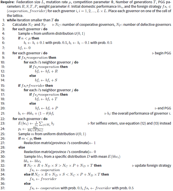
The model settings above imitate the typical yardstick competition in politics (Shleifer 1985; Besley & Case 1995) and we are interested in the simulation outcome for such model settings in a cellular game. The algorithm for the baseline model is given in Algorithm 1. We envisage the following questions according to the simulation results:
- Will democracy and yardstick competition lead to better performances of local governments in general?
- What spatial characteristics of government performances will emerge given different initial settings?
 |
Simulation results
Under different \(bc_i\) distribution
As discussed in the previous section, the distribution of \(bc_i\) may take various forms. We propose different types of the distribution and then test the outcomes under these \(bc_i\) distributions.
We generally consider uniform distributions in the following subsection. All the other distributions that \(bc_i\) follows should meet the basic requirements that the mean of the distribution should be \(E(bc_i)\), if we assume that voters' estimation of the challenger's performance is appropriate. The assumption holds for rational voters in the long term: if the distribution's mean is larger or smaller than \(E(bc_i)\), voters will eventually notice this discrepancy and then adjust their estimation of \(bc_i\) to equal the mean value.
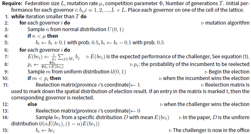
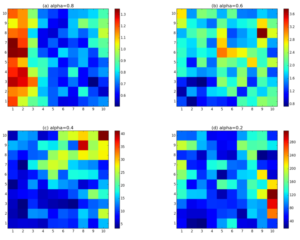
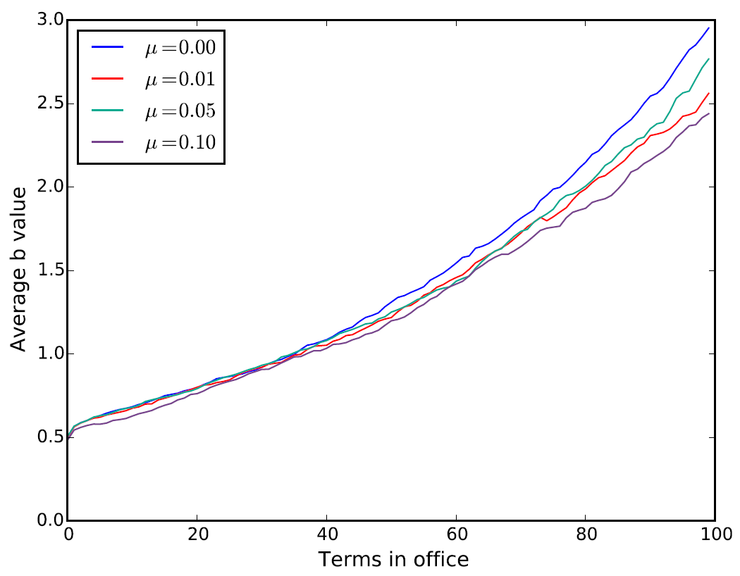
The main result of the simulations in Figure 1 is that the average b value across the federation (i.e., the federal average performance of governors) will increase over terms in office under these (bc_i) distributions. In particular, the value of \(\alpha\), representing the potential range of the distribution, is positively related to the average b value in general. A larger range of \(bc_i\), namely the value of \(\alpha\), will provide voters with a larger range of the challenger’s possible performance. Due to the voting system and yardstick competition, the newly elected governor with larger \(bc_i\) will enjoy support from voters, and the newly elected governor with lower \(bc_i\) will lose her governorship soon after, so despite the risk of electing an incompetent governor, voters will benefit from the uncertainty of the challenger’s performance in the long run.
Result 1: In a certain range, the larger the range of the challenger’s possible performance, the better the overall performance of the governors in the federation.
It is worth noting that in Figure 1, the time length we used in the simulation is 100 terms (and it would be even larger in the rest of the paper), which is equivalent to 400~600 years in reality. Obviously, a continuous 400-year election has never appeared in history, but we run the simulation for at least 100 steps to ensure the robustness of the result and show more details for the evolutionary paths.
Under different initial distributions of \(b_i\)
One of the major advantages of the cellular automata is to enable readers to observe the spatial characteristics directly. We are interested in the spatial distribution of governor’s performance in the model of gubernatorial election under different initial settings.
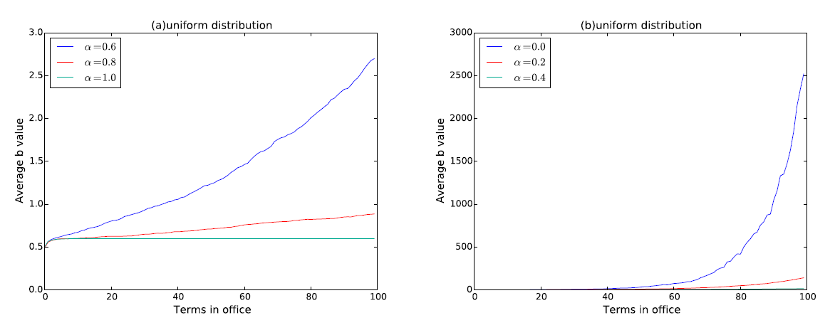
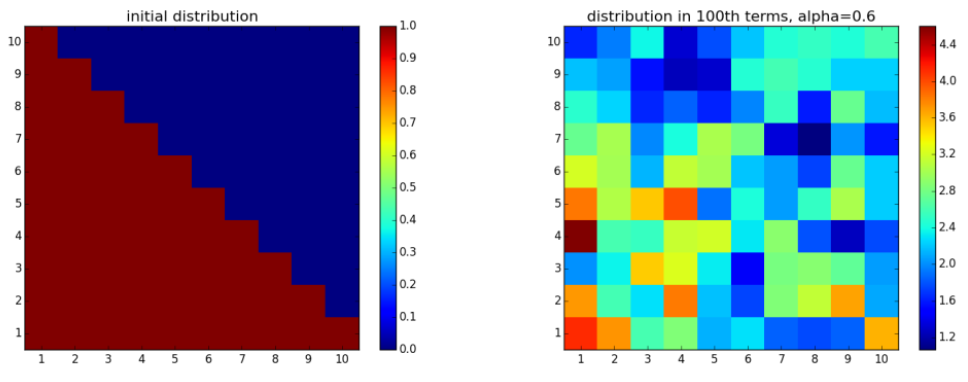
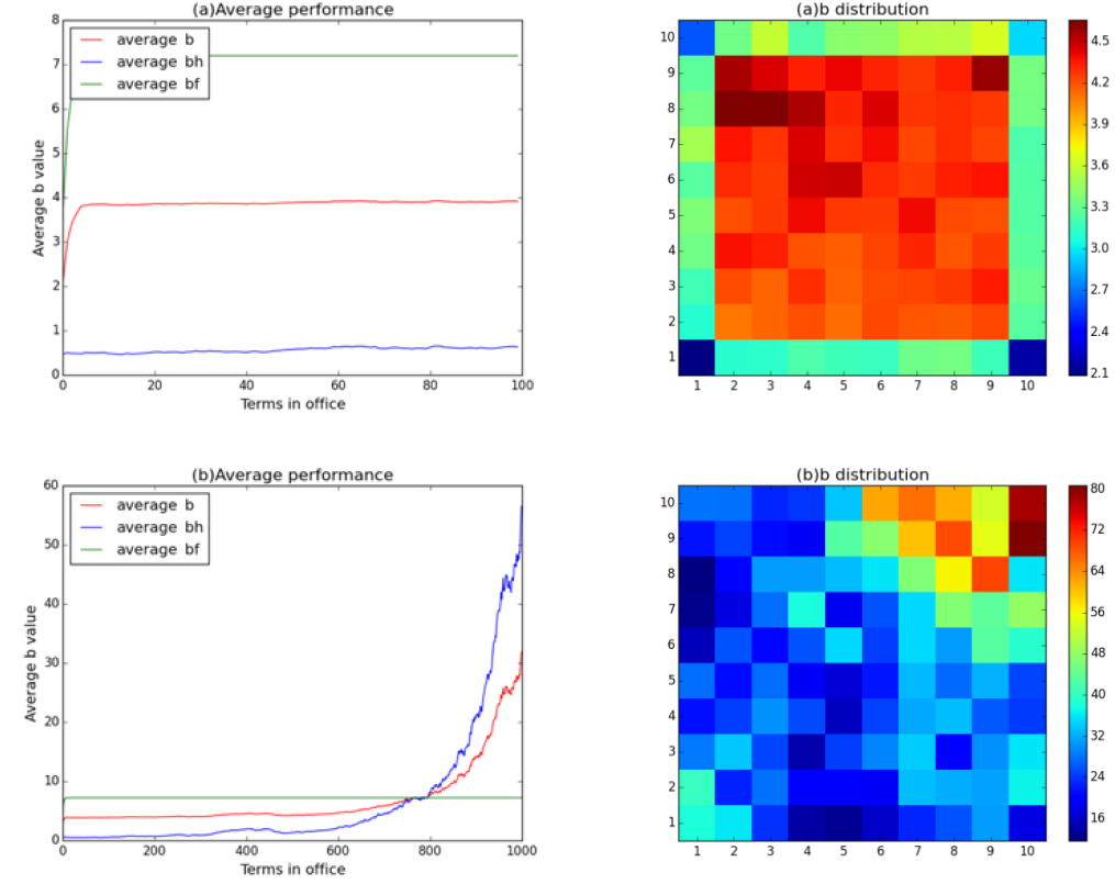
Figure 2 shows the simulation outcomes in the 100th term (right column) and the corresponding initial distributions (left column). It is observed from the outcomes that high-level- and low-level-performance provinces are clustered in different regions in the panel, resulting in the gradient of governor’s performance across the federation. The initial settings (left column of Figure 2) are randomly generated to describe the situation where each governor was initially given a random performance \(b_i \in [0,1]\). By comparing the initial distribution and the simulation outcome, we cannot assert any links between the initial distribution of governors’ performances and the outcome; thus, we believe that the random fluctuation creates the gradients of governor performances from the initial randomness.
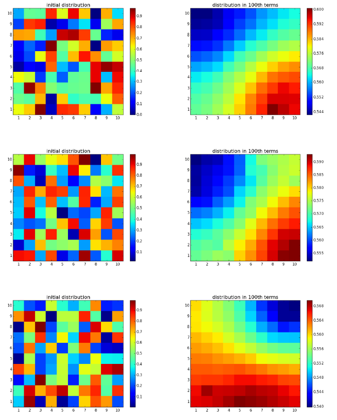
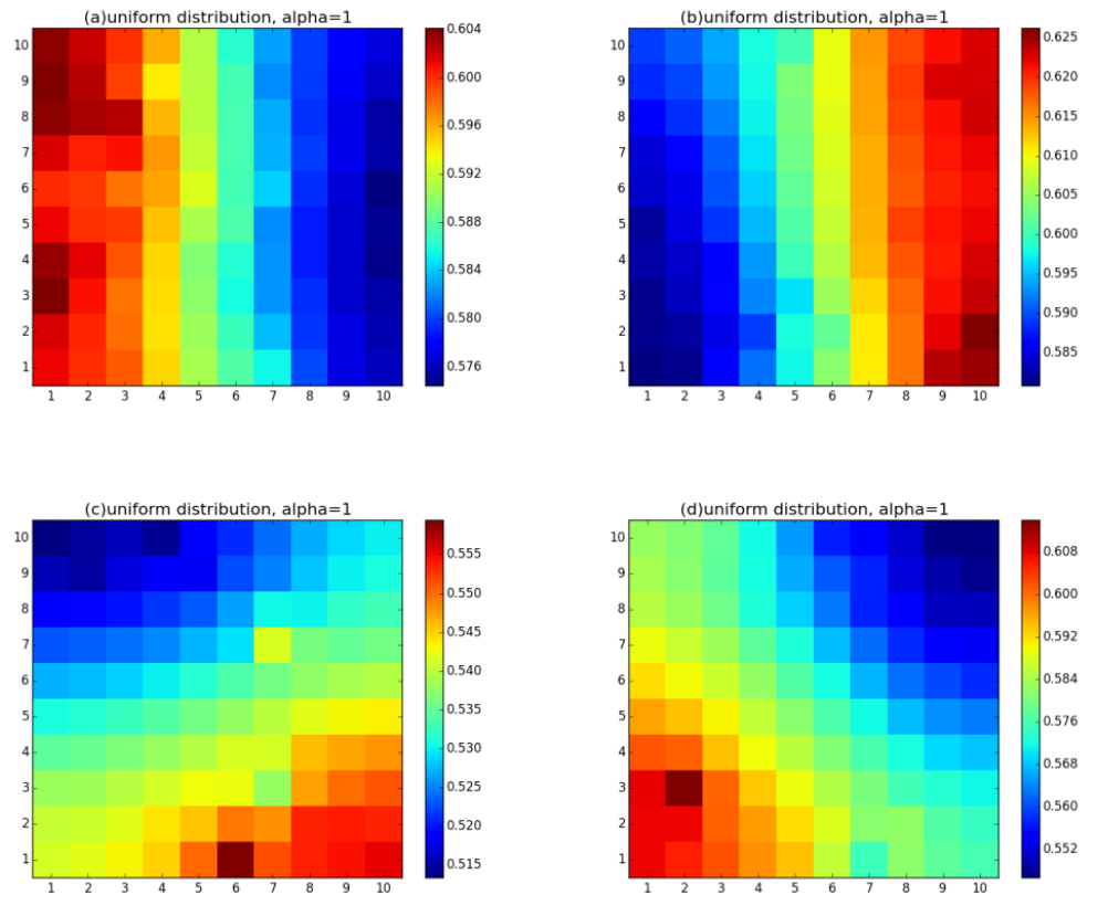
Figure 3 shows the 4 types of phenomena of agglomeration and gradient. More than 4 outcomes of agglomerations can be witnessed in the simulations[1], but the spatial characteristic of clusters still holds.
The basic intuition beneath the phenomena of performance gradient follows the key idea in yardstick competitions: a governor may lose incentives to improve her administrative ability or to embark on reforms if her neighbouring provinces are also suffering from their governors’ bad performances since the voters may downgrade their expected ratings on the incumbents according to the decrease in the welfare of the neighbouring provinces. In the same fashion, a governor whose neighboring provinces exhibit better development level faces great pressure to improve his performance in order to survive the next election.
The setting \(bc_i = E (bc_i)\) indicates that there is no uncertainty about the challenger’s performance, so voters are aware that the next governor, if the challenger is elected, will be of the average level of performance of their neighbouring governors. The lack of uncertainty drives the performance distribution into high agglomeration. Once the uncertainty of the challenger’s performance emerges, the spatial characteristic of agglomeration disappears and turns into disordered patterns gradually because of the increasing uncertainty (see Figure 4). The value of \(\alpha\) indicates the range of performances of the challengers.
To compare with the spatial outcomes in Figure 4, we report the simulation results with different initial distributions of governor performances in Figure 5, 6, 7.
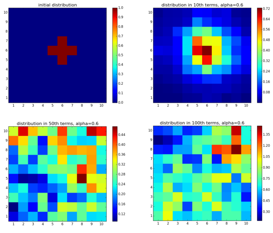
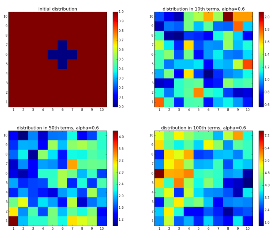
In Figure 5, the initial distribution of governors’ performance represents the division of the federation between the well-governed provinces on the lower left half and the provinces that are suffering from poor governances on the upper right half. In Figure 6, few well-governed provinces are surrounded by the poorly-governed majority, and the distribution goes opposite in Figure 7. It is shown in Figure 5-7 that the initial topology of the distribution will no longer survive after enough long time steps. Instead, the heterogeneity in governors’ performances may increase over time. For example, in Figure 7, the initial difference in performance between the best and worst governor is 1.0, and the difference climbs to more than 1.4 in the 10th term, and more than 5.6 in the 100th term. To conclude, the gubernatorial election improves every governor’s performance, but is also likely to widen the gap between provinces.
Result 2: The initial gradient or clusters of governors’ performances will vanish over time due to gubernatorial elections and yardstick competitions, although the heterogeneity in governors’ performances may increase.
In this part, a constraint is made that if \(b < 0.01\), no mutations will occur to ensure \(b \geq 0\). Due to this constraint, if, initially, every governor's \(b\) equals 0, this low-level equilibrium will never be broken. To test the role of mutation, the constraint is relaxed such that mutations can occur for any value of \(b\) and \(b < 0\) is acceptable. The simulation results under the relaxed condition are shown in Figure 8.
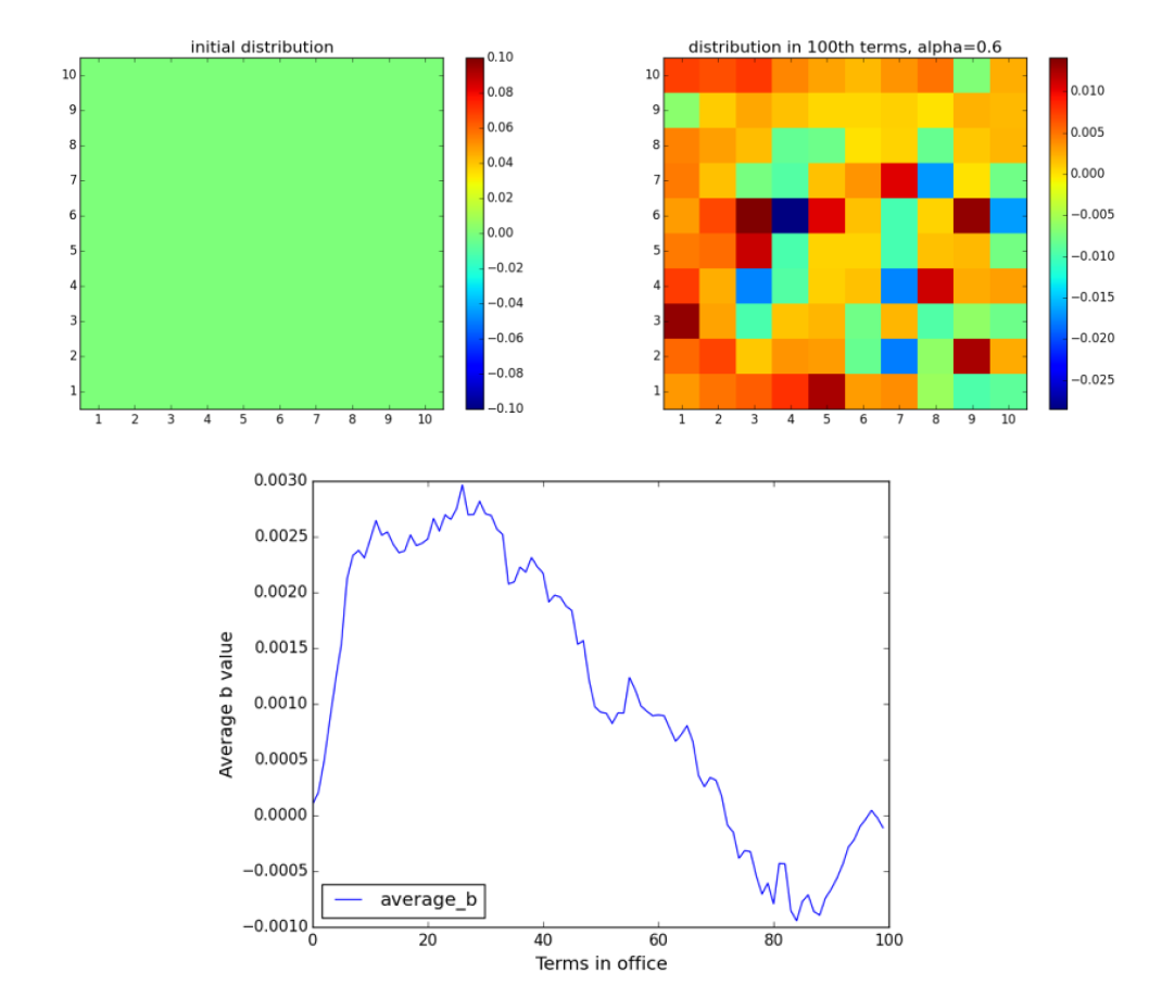
Figure 8 shows that even at a very low mutation rate (\(\mu = 0.01\)), fluctuations will break the low-level equilibrium. Even though the average \(b\) value was finally less than 0, the federation enjoys comparatively high average \(b\) values before the 60th term.
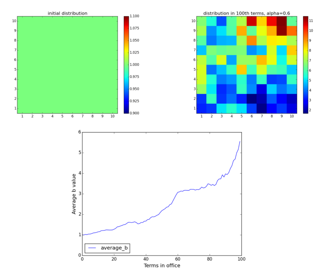
Similarly, the process of the evolution of \(b_i\) when, initially, every governor obtained 1 is also based on mutations. The simulation result is shown in Figure 9.
Robustness check
Robustness checks on various parameters (\(L\), \(\mu\) and \(\Phi\)) and iterations (terms in office) are performed to ensure the power of the model. The simulation results in previous sections are robust with respect to the initial settings. Several meaningful test results are reported in this subsection.
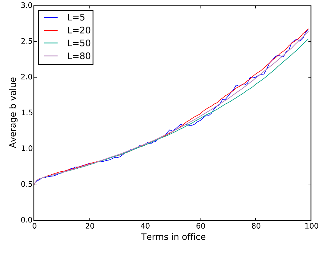
It is well known in the field of innovation economics that a larger number of lower-level jurisdictions will result in a higher overall performance of policies in a federal system when policy innovation and intimation are conducted by jurisdictions (Linge 2008; Saam & Kerber 2013). To investigate the role of the number of provinces (\(N = L * L\)) in the election, we test the hypothesis in our gubernatorial model by performing a robustness check on the parameter \(L\).
In contrast to the classical outcome in innovation economics, Figure 10 shows that the number of provinces is not an important factor involving the evolution; that is, we cannot predict the comparative outcomes of average performance, ceteris paribus, from the numbers of provinces. The absence of the higher-number-of-provinces advantage in the gubernatorial game may result from the voter’s bounded rationality in information: one can only observe the b values of one’s neighbours, and thus other members of the federation cannot affect the election directly.
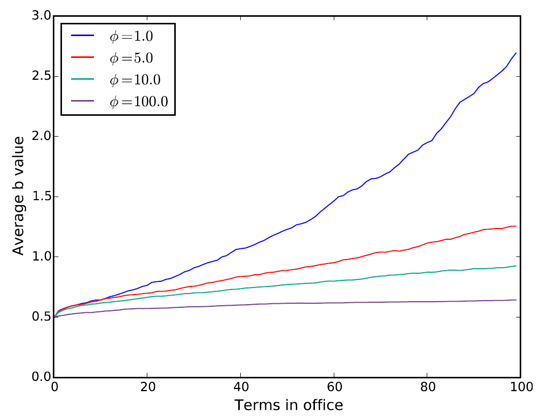
The value of \(\Phi\) measures the intensity of yardstick competitions at the province level (Bodenstein & Ursprung 2005), where \(\Phi\)=1 denotes the complete yardstick competition, and a higher \(\Phi\) denotes an incomplete competition with an incumbency advantage between governors.
Figure 11 shows the simulation of models with different \(\Phi\). The more intensive the yardstick competition (i.e., smaller \(\Phi\)), the higher the long-term overall performance of all governors. When \(\Phi = 100\), where the effect of yardstick competition is small enough, the average \(b\) value increases slightly during the 100 terms. It is possible to predict the extreme outcome in which the overall performance undergoes no change if \(\Phi\) goes to infinity. The simulation result signifies the importance of the conditions affecting the value of \(\Phi\) including incumbency advantage, free flow of information across provinces, and the comparability of the performances between governors.
The robustness check with respect to the mutation rate \(\mu\) implies that mutation does not significantly affect the overall performance (Figure 12), except for the situations in Figure 9 and 9.
Result 3: The number of provinces and the value of the mutation rate are not the main contributors to the evolution of the overall performance in a federation. However, mutations may be the driving force to break the low-level equilibrium.
Further discussion: Geometric random walk model and simulation length
In the previous subsections, we have described the dynamics of the average performances of governors by figures. The topology in these figures suggests that there is a resemblance of average performance histories to a geometric random walk. The model of random walk has been widely used in financial time series and other social sciences to describe and forecast the related process (Voit 2005; Barrat et al. 2008). In the geometric random walk, the natural logarithm of the process is assumed to walk a random walk (Nau 2014). To illustrate the relations between the evolutionary path of government performances and geometric random walk, we plot the natural logarithm of the average b value from a typical simulation result of 500 periods.
The average b value plot in Figure 13, just like any other previous plots, presents a similar pattern of exponential growth with occasional oscillations. The log plot of average b values, in a rough term, resembles a linear trend fitting. In Figure 14, the first difference of logged series can tell us more about the statistical feature of the process. It is easy to tell that there is a drift different from zero in the diff-log plot. Actually, the mean change is 0.015297, while the standard deviation is 0.020636, which means that from one term to the next, the index grows on average by 1.5%.
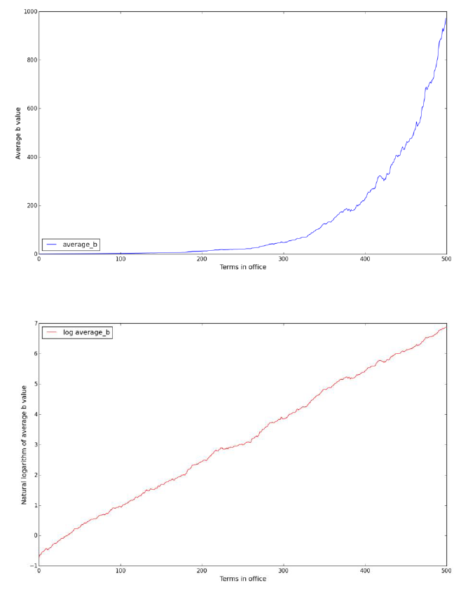
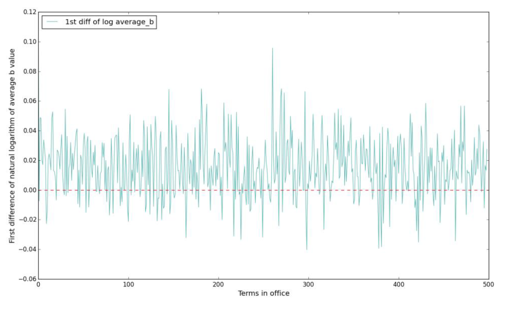
The pure noise pattern of the diff-log plot indicates that the geometric random walk model is a simple but efficient way to model the process (for a discrete geometric random walk \(\{X_t\}\), its diff-log \(\log X_{t + 1} - \log X_t\) for all \(t\) is a white noise \(\xi\) by definition). In particular, the evolution of government's performance can be modeled as:
| $$\acute{b} (t) = e^{x (t)}$$ | (3) |
| $$x (t) = x (t - 1) + \xi+ c$$ | (4) |
The memoryless property of the geometric random walk model can help us simplify the simulation. The property illustrates that the changes in natural logarithm from one term to the next is not related to the history of the process, which permits the expected growth in average b for all the terms followed by. Therefore, the average performance of governments will continue to grow, although some short-term volatility may be observed. The memoryless property can simplify our following practice: we no longer need to perform too many simulation steps to permit the robustness of the results.
Models with inter-jurisdictional affairs
Setup
The impact of foreign countries’ policies and incumbent’s foreign policies on the presidential election has enjoyed lasting interest among scholars (Risse-Kappen 1991; Smith 1996; Small 1996; Mead 2002), but few researchers have focused on the relations between inter-jurisdictional policies and gubernatorial elections. Regardless of the home affairs such as local tax policies, lower-level jurisdictions, if enjoying far-reaching autonomy as the German Bundesländer or the Belgian regions, are also responsible for dealing with foreign affairs with their neighbours and other members of the federation. As pointed out by Halperin et al. (2006), foreign issues definitely affect the presidential election in the United States. The inter-jurisdictional policy (executed inside the federation) not only affects the welfare of the jurisdiction but also plays an exogenous role in the calculation of other member states’ welfare, especially for the jurisdiction’s neighbours. Obviously, jurisdictions will receive more policy externality impacts from their neighbours than other member states, resulting from the externality of public goods, whether natural (e.g., water resource sharing by jurisdictions) or artificial (e.g., a hospital also serving the neighbouring citizens), and direct interactions such as trade, aid or even conflicts.
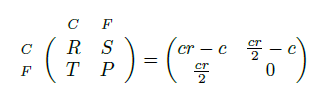
As sovereign entities within the federal system, in our model, each province has its own authority to deal with inter-jurisdictional affairs, although the authority may be restricted and supervised by the federal government. In this section, we model the inter-jurisdictional affairs with a conventional evolutionary public goods game (PGG) involving two neighbouring governors as players. One good example is the construction of cross-provincial public infrastructure, which is beneficial to both provinces. We assume that the governor can play either ‘Contribute (C)’ or ‘Free ride (F)’ as her foreign strategy. The payoffs for the contributor and free rider are:
| $$P_C = \frac{cr N_c}{2} - c$$ | (5) |
| $$P_F = \frac{cr N_c}{2}$$ | (6) |
| $$bf_i = \frac{1}{n_i} \sum_{j \in M_i} \text{Payoff}_{ij}$$ | (7) |
For simplicity, in this section, we suppose that the governor will be consistent in choosing the strategy: after choosing C or F to deal with foreign affairs, the governor will play this strategy with each of his neighbours and will not change the strategy as long as the governor is in office. This constraint will be relaxed in later sections.
The payoff from inter-jurisdictional affairs is also considered to be a composition of the governor’s performance; that is:
| $$b_i (t) = \theta bh_i (t) + (1 - \theta) bf_i (t) $$ | (8) |
The challenger's performance in inter-jurisdictional affairs, if elected, will be more complicated than in home affairs as defined in the baseline model. First, we assume that the voters cannot disengage \(bf_i\) from \(b_i\); the voters can only observe the overall performance of the governor. Since the voters cannot monitor \(bf_i\) directly, they are indifferent to foreign strategies and have no moral preference on either strategy. In this case, the challenger is free to choose her C or F in the PGG. For the dynamics of the foreign strategies, we assume that the elected challenger (whose term in office is \(t\)) is politically rational, and she makes the inter-jurisdictional decision according to her neighbouring provinces' strategies in term \(t - 1\) to maximize \(bf_i (t)\), although the neighbouring provinces' strategies may alter in term \(t\). Pre-tests indicate that more attention should be paid to the behaviors of governors when they are indifferent to playing C and F (i.e. Playing C and F will result in the same payoff). If we force the governor to accept F when she is indifferent to both strategies, then the equilibrium would be that every governor plays F. Thus, we assume that when the governor is indifferent between C and F then she will randomly choose C or F with equal probabilities.
The probability of a challenger obtaining the governorship is the same as equation (1) and (2), and
| $$bc_i \quad U ( \alpha E (bc_i), (2 - \alpha) E (bc_i) ) $$ | (9) |
 |
Selfish voters
In this subsection we continue to study the voters who are set to care about their own provinces. We call them selfish voters, whose idea can be traced back to the basic utility hypothesis for the calculus of voting (Riker & Ordeshook 1968). For selfish voters, their utility of voting is independent of other provinces, suggesting that their voting behaviour is determined by their governor’s performance only. The selfish voters are designed to behave in the same manner as the voters described in the baseline model, and the only difference is that the selfish voters in this particular subsection consider the entire performance (i.e. \(b_i (t) = \theta bh_i (t) + (1 - \theta) bf_i (t)\)) of the governors and challengers, rather than the performance of home affairs alone.
Figure 15 depicts the evolutions of both overall performances of governors. Under these initial settings and update formulae, all governors will choose the strategies of F, and thus \(bf_i = 0\) for \(i = 1,2,\dots,N\), which is a common result of the public goods dilemma (Olson 1965; Hardin 1997; Dionisio & Gordo 2006). In addition, the evolutionary path of the performance in home affairs \(bh_i\) is similar to the path of \(b_i\) in the baseline model (see Figure 1). To be particular, for Figure 15(b), the drift of the geometric random walk model is 0.016014. Since all governors play F infinitely, the game with inter-jurisdictional affairs does not differ from the baseline model, and thus the evolution of the performance in home affairs follows the update dynamics in models without foreign affairs.
Since each inter-jurisdictional game only involves 2 players, we can simply conclude the payoffs in the following payoff matrix:
 |
In this simulation, we can compute the payoff matrix with the parameters given in Figure 1: \(R=0.5\), \(S=-0.25\), \(T=0.75\), \(P=0\). Note that the payoff of the free rider in the unilateral contribution, \(T\), is larger than the payoff for mutual contribution, \(R\). Intuitively, we test the simulation result for \(T < R\). when the best payoff for a free rider (\(T\)) is less than the payoff for a contributor when mutual contributions occur (\(R\)).
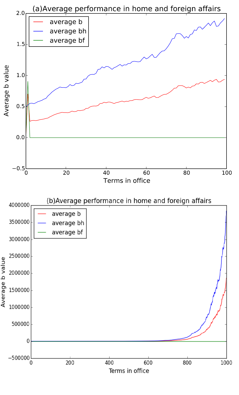
Figure 16 shows the reversal of strategies when \(R=2\), \(S=0.5\), \(T=1.5\), \(P=0\). The federation has reached an equilibrium where every governor plays C in every term (not shown due to the limitation of length). Meanwhile, the overall performance in home affairs reaches the low-level equilibrium in the first 100 terms compared with the simulation in Figure 15. Simulation (a) b distribution (top right of Figure 16) portrays the diamond-like spatial distribution of the performance \(b_i\), which is due to the lack of the periodic boundary condition (see Sections 2.1-2.8). Fewer yardstick competitions for a governor will lead to lower performances in borderlands. When \(R>T\), governors have no incentive to play F anymore; thus more neighbours means more inter-jurisdictional games and more payoffs.
We find that given enough long terms the performance in home affairs will experience unexpected growth after certain periods (the turning point in Figure 16(b) is 600 terms). Comparing Figure 15 and 16, the late development of governor's performance when \(R<T\) cannot catch up with the development when \(R>T\). Note that in the game with inter-jurisdictional affairs, the voters cannot disengage \(bf_i\) from \(b_i\); the voters evaluate the challenger's performance according to the average value of the neighbouring governors' overall performance \(b_i\), rather than the performance in home affairs only (\(bh_i\)). When R>T, all governors play C, and thus \(bf_i\) reaches the maximal value for each \(i\). In this circumstance, the gap between incumbents with low and high \(bh_i\) is relatively reduced because the common high-level \(bf_i\) has compensated part of the difference between governors. Consider an extreme case when \(bf_i = \inf\); then the voting systems lose all the incentive to promote \(bh_i\) since the governor's performance in home affairs is completely ignored. Namely, in the first 600 terms, the low-level equilibrium trap for performances in home affairs can be ascribed to the emergence of the high-level equilibrium for performances in foreign affairs. The payoffs from inter-jurisdictional games are large enough for the voters to ignore the performance inside the province, and therefore the evolution of \(bh_i\) stops. To verify this assumption, we make the following robustness checks with respect to the value of \(\theta\), the weight of home affairs when evaluating the governors in Figure 17.
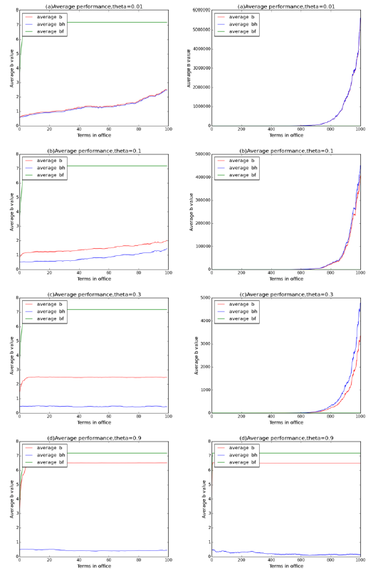
The simulations in Figure 17 indicate that a lower weight of inter-jurisdictional affairs in evaluating the governor will lead to better governor performances in home affairs. This conclusion is widely applied in politics when public officials try to create foreign emergencies to divert voters’ attention from domestic affairs. However, this low-level equilibrium will be eventually broken in the future even if the weight of foreign affairs is large. The breakthrough may be ascribed to the accumulation of time, which eventually induce some good-performance governors, and once the average \(bh_i\) breaks the threshold created by foreign affairs, nothing can act as a brake on growth. This process may explain the exponential growth of \(bh_i\) in some subplots of Figure 17.
Once voters observe \(bh_i\) and \(bf_i\) separately, the foreign affairs no longer influence the governor's performance in home affairs, and the simulation results will be similar to the simulation results in Sections 2.1-2.35.
Result 4: A lower weight of inter-jurisdictional affairs in evaluating the governor will lead to the governor’s better performance in home affairs when all governors are free riders.
Selfless voters
In the previous sections, we took it for granted that all the voters were rational and selfish, and their behaviours were entirely based on the welfare of their own provinces, taking neighbouring provinces’ welfares as references. Additionally, in most studies on yardstick competitions or gubernatorial elections, the jurisdiction is isolated from the federation, focusing on a single governor’s political performance but not on the spatial characteristics covering other jurisdictions. Moreover, the behaviours of voters in previous studies were the univariate functions of an individual’s own utility or the local social welfare (McNutt 2002). This assumption is taken for granted in presidential electoral studies, indicating that voters care about foreigners only if foreigners can influence their own country (e.g., via invasion, annexation). However, at the level of gubernatorial elections, local voters often have social preferences (Hoffman et al. 1996) which may overflow to neighbouring jurisdictions due to the recognition of national identity in the same federation or the close relations between voters and neighbouring citizens. In the research field of cooperation, scholars have found that taking neighbours’ payoffs into consideration could be the driving force for the emergence of cooperative behaviours in network games (Chen et al. 2008, Li et al. 2016). It is appropriate to transplant the altruistic characteristics for players from the evolutionary cooperation literature to the voters as one of the alternatives for voter’s type.
We first assume that all voters are of bounded selflessness; namely, they only care about the von Neumann neighbourhood. The adjective ‘bounded’ here means that the local voters show no interest in the welfare of provinces that share no boundaries with their own province of residence. The assumption of boundless selflessness is only appropriate for the presidential election, and therefore bounded selflessness is a remarkable feature of gubernatorial elections.
Following the tradition of philosophy, we consider the following two types of selfless voters: The Utilitarian voter (Bentham 2007) and the Rawlsian voter (Rawls 1971). Utilitarian voters evaluate the governor according to the summation of the neighbourhood’s (including their own province) performances in both home and foreign affairs:
| $$W_i^U (t) = \sum_{j \in Q_i} b_j (t)$$ | (10) |
| $$W_i^R (t) = \min (b_j (t)) \text{,} \quad j \in Q_i $$ | (11) |
Although the selfless voters predict the challenger's potential using the average value of neighbouring provinces' \(W_i^U\) or \(W_i^R\), the actual distribution of challenger’s performances in home affairs still follows the distribution \(U ( \alpha E (bhc_i), (2 - \alpha) E (bhc_i) )\), as in the previous sections. Since the voters cannot distinguish the performance in home affairs from foreign affairs, they can only evaluate the challenger using the average performance in both affairs of all neighbouring governors, but it is only accurate to estimate the challenger's performance in home affairs according to its neighbours because the challengers will choose foreign policies based on the policies of the incumbents nearby in the last term. Therefore, the existence of foreign affairs will induce the information asymmetry in voters as side effects even if \(\theta = 0\).
Equations 10 and 11 have the implication of justice, which means the voters are more sensitive to the welfare of neighbouring citizens. This assumption of justice is based on the fact that the governor’s strategy in inter-jurisdictional affairs can affect the welfare of neighbouring provinces; thus, the voters should also be responsible for their neighbours’ welfare when electing their own governor. However, the local governor cannot affect the welfare of non-neighbour provinces, so local voters will ignore the non-neighbour citizens.
The dynamics of the election mirror Sections 2.42-2.50; only the expression for \(E (bc_i)\) changes for different types of selfless voters. For Utilitarian voters:
| $$E^U (bc_i) = \frac{1}{n_i} \sum_{j \in Q_i} W_j^U$$ | (12) |
| $$E^R (bc_i) = \min ( W_j^R (t) ) \text{,} \quad j \in Q_i$$ | (13) |
| $$P_i^x (t) = \frac{\Phi W_i^x (t)}{\Phi W_i^x (t) + E^x (bc_i)}$$ | (14) |
Conducting simulation models of elections with Utilitarian voters in Figure 18(a) results in the situation in which all governors play \(F\) when \(R<T\). Unexpectedly, except for the public goods dilemma that emerged in the elections with selfish voters (see Section 2.51), the Utilitarian voters have created a low-level equilibrium for average performance. Although the patterns for (a) and (b) look different both simulations in (a) and (b) can be described by geometric random walk models with negative drifts (\(bh (t) = e^{x(t)}\), \(x (t) = x (t - 1) + \xi +c\)). For \(R<T\), \(c =\)-0.001899 and for \(R>T\), \(c=\)-0.001343. The drifts tell us that regardless of the relations between \(R\) and \(T\), the average performance will decrease continuously and slowly in foreseeable future. The major difference in (a) and (b) should lie in the foreign affairs. Compared to Figure 18(a), Figure 18(b) exhibits a similar outcome for governors’ performances. In fact, there is nearly no difference between the evolutionary paths of average bh values in (a) and (b).
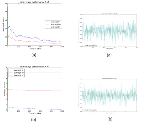
Figure 19 shows the results for Rawlsian voters. When \(R<T\), although all the governors' performances in foreign affairs are zero, the performances in home affairs exhibit a surprisingly exponential growth. When \(R>T\), the simulation results are not consistent: most cases report the flat evolutionary paths as in Figure 18(b), but different types oscillations may occur randomly over time. Compared to the outcomes of the Utilitarian voters, the overall performances are significantly promoted when \(R>T\) but reduced when \(R>T\) in a federation with Rawlsian voters.
Result 5: Altruistic voters will lead to lower performances of governments regardless of the types of altruistic voters (Utilitarian or Rawlsian) and the relations between R and T.
Utilitarian voters evaluate challengers by the welfare of neighbours’ neighbours, and Rawlsian voters vote according to the local minimal performance: the concern of selfless voters is far from the welfare of their own province. Thus, voters no longer stand for the interest of the local citizens and governors no longer work for local welfare. This results in the tragedy of kindness as stated in Result 5.
For the Rawlsian voters, consider a province k with local minimal performance; according to Equations 2, 13 and 15, we have bk=E(bck) and thus the probability of governor k’s reelection will be:
| $$P_k = \frac{\Phi b_k}{\Phi b_k + E (bc_k)} = \frac{\Phi}{\Phi + 1} = 0.5$$ | (15) |
Thus, given enough terms, the governor is highly likely to fail the election, and since the challenger's performance in home affairs follows the uniform distribution ranging from \(0.6 E (bhc_k)\) to \(1.4 E (bhc_k)\) where \(E (bhc_k) > bh_k\). Once the challenger is reelected, the province \(k\) will enjoy better performance with relatively high probability. Similarly, if province \(z\) is one of \(k\)'s neighbours, we still have \(P_z = \frac{1}{\Phi + 1}\) regardless of \(b_z\). This situation causes many oscillations of the evolutionary paths.
Conclusion and Discussion
Although not uncontroversial, the application of cellular automata simulation in electoral studies captures many aspects of democracy at the gubernatorial level. In contrast to the traditional orientation of political studies, the evolutionary and spatial studies on elections in this paper place much weight on the process and transformation of the social welfare, which is expressed as the governor’s performance driven by the voting system. The foregoing exercises of simulations have illuminated several problems concerning the evolution of governors’ political performances in provinces.
Both yardstick competition and politics have been and remain today popular subjects among scholars, but most papers involving in these two topics focused on tax setting/mimicking (e.g. Besley & Case 1995; Bordignon et al. 2003; Allers & Elhorst 2005) and provision of public services (e.g. Revelli 2006; Terra & Mattos 2017), rather than the basic intuition beneath the election outcomes, and its relations with both voter’s behaviours and cross-border interactions. Although rooted in the context of Tullock (1980) and the Bodenstein-Ursprung (2005) models for fiscal choice/ economic behaviours, this paper offers proofs of some intuitive statements in the gubernatorial elections in the environment of a simple spatial gubernatorial game.
The main purpose of this paper is to suggest a method of computer simulation to model the dynamics of electoral outcomes. Following the previous observations, we propose the following results concerning the governors’ performances. From the side of governors, the following three findings are worth noting: (i) larger range of the challenger’s performances will induce better overall performance of governors in the entire federation; (ii) there is no evidence supporting that the initial distribution of governors will affect the overall and specific states’ performance in the long run; and (iii) the mutation of governors’ performance drives the entire federation out of a stable equilibrium, and a fiercer competition among the governors will lead to a better overall performance. From the side of the voters, the first finding is that a lower weight from the voters evaluating the inter-jurisdictional affairs induces better governor performance when all governors are free riders. Moreover, we find that altruistic voters will trap the performance into a lower level.
Although some conclusions are commonly observed in political practices, others seem to be meaningful only with highly strict assumptions. Keeping to these conclusions, we may conjecture the possible potential of democratic systems. More precisely, we underline the importance of voters’ perception of both the incumbent and the challenger in the evolution of democracy. The cardinal difference between selfish voters, Utilitarian voters and Rawlsian voters is not in their moral virtues; the difference lies in the methods of evaluating the incumbent and predicting the challenger. Notwithstanding that we have analysed three types of voters, the most efficient method to promote politicians’ performance is to ensure the information transparency of the candidates for the governorship or presidency. In this paper, the information asymmetry or the lack of information transparency is represented by the mismatch between challenger’s performances and voters’ perceptions and the impossibility of distinguishing incumbents’ performances in home and foreign affairs. The asymmetry increases the uncertainty of the electoral results and therefore reduces the power of democracy. Such settings of asymmetry fit the reality of voters. American voters were found to base their assessments largely on the recent economic trends (Alesina & Rosenthal 1995; Hansen 1999) and unemployment rate (Dua & Smyth 1993), although the incumbents are not directly responsible for the periodic shocks to the economy. Gubernatorial politics turn to unpredictable disorders if the voters place too much emphasis on local conditions that governors cannot control. If the voters are all "naïve retrospective” (Alesina & Rosenthal 1995), then in our simulation model, the voters’ judgement of the incumbent and the expectations of the challenger will not be related to the abilities and performances of the candidates: it is similar to buying bulls by judging the milk.
Admittedly, in politics, we are far from a complete description of the real-world gubernatorial election. Due to the absence of presidency in the model, we did not capture the effect of federal government and presidential election on gubernatorial election. Moreover, games involving inter-provincial affairs are much more complicated than simple public good games, and the payoff from inter-provincial affairs is not the only foreign factor affecting the election: sometimes the local recognition, citizens’ discontent and hostility among provinces due to the interactions between governors may change the election outcome. Even with these defects, the spatial model we establish in this paper may be helpful in understanding the evolutionary process of government performance in gubernatorial elections in various circumstances. To proceed forward, we suggest further geopolitical studies based on the framework, emphasizing the spatial features and evolution of the democratic system.
Notes
- There are in general two types of distribution: diagonal gradient (Figure 3 (c) & (d)) and vertical/horizontal gradient ((a) & (b) are of horizontal gradient distribution), adding the direction of the gradient, there will be 8 classifications. We have picked 4 examples in Figure 3 to avoid redundancy.
References
ALESINA, A., & Rosenthal, H. (1995). Partisan Politics, Divided Government, and the Economy. Cambridge: Cambridge University Press. [doi:10.1017/CBO9780511720512]
ALLERS, M. A. (2012). Yardstick competition, fiscal disparities, and equalization. Economics Letters, 117(1), 4-6.
ALLERS, M. A., & Elhorst, J. P. (2005). Tax mimicking and yardstick competition among local governments in the Netherlands. International Tax and Public Finance, 12(4), 493-513. [doi:10.1007/s10797-005-1500-x]
ATKESON, L. R., & Partin, R. W. (1995). Economic and referendum voting: A comparison of gubernatorial and senatorial elections. American Political Science Review, 89(01), 99-107.
BARRAT, A., Barthelemy, M., & Vespignani, A. (2008). Dynamical Processes on Complex Networks. Cambridge: Cambridge University Press. [doi:10.1017/CBO9780511791383]
BENTHAM, J. (2007). An Introduction to the Principles of Morals and Legislation. Mineola, NY: Dover.
Besley, T., & Case, A. (1995). Incumbent behavior: Vote seeking, tax setting and yardstick competition. American Economic Review, 85(1), 25-45.
BESLEY, T., & Smart, M. (2007). Fiscal restraints and voter welfare. Journal of Public Economics, 91(3-4), 755-773.
BRETON, A. (1998). Competitive Governments: An Economic Theory of Politics and Public Finance. Cambridge: Cambridge University Press.
BRÜLHART, M., & Jametti, M. (2006). Vertical versus horizontal tax externalities: an empirical test. Journal of Public Economics, 90(10), 2027-2062.
BODENSTEIN, M., & Ursprung, H. W. (2005). Political yardstick competition, economic integration, and constitutional choice in a federation. Public Choice,124(3-4), 329-352. [doi:10.1007/s11127-005-2051-5]
BORDIGNON, M., Cerniglia, F., & Revelli, F. (2003). In search of yardstick competition: a spatial analysis of Italian municipality property tax setting. Journal of Urban Economics, 54(2), 199-217.
CHEN, X., Fu, F., & Wang, L. (2008). Promoting cooperation by local contribution under stochastic win-stay-lose-shift mechanism. Physica A: Statistical Mechanics and its Applications, 387(22), 5609-5615. [doi:10.1016/j.physa.2008.05.043]
CHIRINKO, R. S., & Wilson, D. J. (2011). Tax competition among US states: racing to the bottom or riding on a seesaw?. CESifo Working Paper No. 3535.
COSTA-FONT, J., De-Albuquerque, F., & Doucouliagos, H. (2015). Does inter-jurisdictional competition engender a “Race to the Bottom”? A meta-regression analysis. Economics & Politics, 27(3), 488-508. [doi:10.1111/ecpo.12066]
DEVEREUX, M. P., Lockwood, B., & Redoano, M. (2007). Horizontal and vertical indirect tax competition: Theory and some evidence from the USA. Journal of Public Economics, 91(3), 451-479.
DIONISIO, F., & Gordo, I. (2006). The tragedy of the commons, the public goods dilemma, and the meaning of rivalry and excludability in evolutionary biology. Evolutionary Ecology Research, 8(2), 321-332.
DUA, P., & Smyth, D. J. (1993). Survey evidence on excessive public pessimism about the future behavior of unemployment. Public Opinion Quarterly, 57(4), 566-574.
HANSEN, S. B. (1999). “Life Is Not Fair”: Governors' job performance ratings and state economies. Political Research Quarterly, 52(1), 167-188.
HALPERIN M. H., Clapp P., & Kanter, A. (2006) Bureaucratic Politics and Foreign Policy. Washington, DC: Brookings Institution Press.
HARDIN, R. (1997). One for all: The logic of group conflict. Princeton, NJ: Princeton University Press. [doi:10.1515/9781400821693]
HOFFMAN, E., McCabe, K., & Smith, V. L. (1996). Social distance and other-regarding behavior in dictator games. The American Economic Review, 86(3), 653-660.
LI, Y., Ye, H., & Zhang, H. (2016). Evolution of cooperation driven by social-welfare based migration. Physica A: Statistical Mechanics and its Applications, 445, 48-56. [doi:10.1016/j.physa.2015.10.107]
LI, H., & Zhou, L. A. (2005). Political turnover and economic performance: the incentive role of personnel control in China. Journal of Public Economics, 89(9), 1743-1762.
LINGE, G. (2008). Competition Policy, Innovation, and Diversity. Marburg: Tectum Verlag.
NAU, R. (2014). Notes on the random walk model. Technical report, Fuqua School of Business, Duke University, Duke
MEAD, W. R. (2002). Special Providence: American Foreign Policy and How It Changed the World. New York: Routledge.
MCNUTT, P. (2002). The Economics of Public Choice. Cheltenham and Northampton, MA: Edward Elgar Publishing.
OLSON, M. (1965). The Logic of Collective Action: Public Goods and the Theory of Groups. Cambridge, MA: Harvard University Press.
PELTZMAN, S. (1987). Economic conditions and gubernatorial elections. The American Economic Review, 77(2), 293-297.
RAWLS, J. (1971). A Theory of Justice. Cambridge, MA: Oxford University Press.
REVELLI, F. (2006). Performance rating and yardstick competition in social service provision. Journal of Public Economics, 90(3), 459-475.
ROSE-ACKERMAN, S. (1980). Risk taking and reelection: Does federalism promote innovation?. The Journal of Legal Studies, 9(3), 593-616. [doi:10.1086/467654]
RIKER, W. H., & Ordeshook, P. C. (1968). A Theory of the Calculus of Voting. American Political Science Review, 62(01), 25-42.
RISSE-KAPPEN, T. (1991). Public opinion, domestic structure, and foreign policy in liberal democracies. World Politics, 43(04), 479-512. [doi:10.2307/2010534]
SAAM, N. J., & Kerber, W. (2013). Policy innovation, decentralised experimentation, and laboratory federalism. Journal of Artificial Societies and Social Simulation, 16(1), 7: https://www.jasss.org/16/1/7.html. [doi:10.18564/jasss.2123]
SALMON, P. (1987). Decentralization as an incentive scheme. Oxford Review of Economic Policy, 3(2), 24–43. [doi:10.1093/oxrep/3.2.24]
SALMON, P. (2006). "Horizontal Competition among Governments.' In E. Ahmad and G. Brosio (Eds.), Handbook of Fiscal Federalism. Cheltenham UK and Northampton, MA: Edward Elgar, pp. 61-85.
SHLEIFER, A. (1985). A theory of yardstick competition. The RAND Journal of Economics, 319-327. [doi:10.2307/2555560]
STEIN, R. M. (1990). Economic voting for governor and U.S. senator: The Electoral Consequences of Federalism. The Journal of Politics, 52(1), 29-53.
STRUMPF, K. S. (2002). Does government decentralization increase policy innovation?. Journal of Public Economic Theory, 4(2), 207-241. [doi:10.1111/1467-9779.00096]
SMITH, A. (1996). Diversionary foreign policy in democratic systems. International Studies Quarterly, 133-153.
SMALL, M. (1996). Democracy and Diplomacy: The Impact of Domestic Politics in US Foreign Policy, 1789-1994. JHU Press.
TERRA, R., & Mattos, E. (2017). Accountability and yardstick competition in the public provision of education. Journal of Urban Economics, 99, 15-30.
TULLOCK, G. (1980). 'Efficient rent-seeking.' In Buchanan, Tollison and Tullock (eds.), Toward A Theory of the Rent-Seeking Society, College Station, Texas A&M Press.
TSAI, K. S. (2004). Off balance: The unintended consequences of fiscal federalism in China. Journal of Chinese Political Science, 9(2), 1-26.
VOIT, J. (2005). The statistical mechanics of financial markets. Springer Science & Business Media.
WHEATON, W. C. (2000). Decentralized welfare: Will there be underprovision?. Journal of Urban Economics, 48(3), 536-555.
YE, H., Tan, F., Ding, M., Jia, Y., & Chen, Y. (2011). Sympathy and punishment: evolution of cooperation in public goods game. Journal of Artificial Societies and Social Simulation, 14(4), 20: https://www.jasss.org/14/4/20.html. [doi:10.18564/jasss.1805]