
Introduction
In order to attract customers, many retailers are offering a large number of perishable products. This allows them to compete against the more traditional channels that specialize in these items (Adenso-Diaz et al. 2017). Li et al. (2012b) reported that more than 81% of sales in the grocery retail industry in the US in 2009 corresponded to food and beverages, and 63% of those sales were of products with a limited shelf life. This means that more than 50% of this sales channel deals in perishable units. Perishable products often require careful handling, and their limited shelf life requires the implementation of some sort of strategy that manages the spoilage of outdated units. According to Chung & Li (2014), 88% of consumers frequently check expiry dates of perishable product when buying. They prefer to select the fresher units, which provide a higher perception of quality when the units have different expiry dates but the same price (Chung & Li 2013). It is clear that adjusting prices according to product characteristics, instead of adopting a fixed price across the entire shelf life, may increase sales. Therefore, retailers can dynamically change their prices to balance supply and demand based on information such as inventory shelf life and the elasticity of demand.
Price strategies have been extensively studied in perishable industry (e.g., a Cost-plus pricing strategy, a Value-based pricing strategy and an Inventory-sensitive pricing strategy) (Li et al. 2009; Chang et al. 2016). Related research has shown that factors such as cost, uncertain demand, competition and perishable characteristics play a vital role in price setting (Sung & Lee 2000; Shankar & Bolton, 2004; Soni & Patel 2012). Customer preferences (e.g., quality of perishable products, distance to retailers and price of perishable products) have also been recognized as an important factor in modeling people’s economic behavior that is significant to retailers’ pricing strategies (Feldmann & Hamm 2015). These characteristics mean that the pricing problem of perishable products presents a complex, large-scale stochastic modeling challenge. Due to their computational tractability, complex models generally are too difficult to implement in real time. A multi-agent simulation model is considered to be a good instrument for modeling the social interaction of actors (Lee et al. 2014). Chang et al. (2016) proposed an agent-based simulation model to develop a best practice dynamic pricing strategy for retailers. In this model, retailers adjust their pricing strategies according to their current situations. However, their model lacks the ability to perceive customer preferences or to analyze the competitive environment, and it therefore may lead to an incorrect pricing policy for local optimization. To solve this problem, a simulation model that can learn customer preferences implicitly and optimize pricing strategies for perishable products should be created. The Q-learning algorithm is known for its ability to create nearly optimal solutions to problems that involve a dynamic environment with a large state space (Dogan & Guner 2015). Applications of Q-learning in the context of an expert system include real-time rescheduling (Li et al. 2012a), inventory control in supply chain (Jiang & Sheng 2009), and dynamic pricing policies (Tesauro & Kephart 2002). Rana & Oliveira (2015) used reinforcement learning to model the optimal pricing of perishable interdependent products in conditions in which demand is stochastic. However, they did not apply Q-learning to the pricing strategies of different retailers that explicitly model customer preferences in a competitive environment. Moreover, there lack a model-free environment (e.g, a multi-agent system), which includes many influencing factors that are implicitly incorporated into the pricing decisions.
This paper utilizes the advantages of the model-free environment offered by the multi-agent system, and uses the Q-learning algorithm to model the optimal pricing strategy for perishable products considering uncertain demand and customer preference. The model of the virtual market is based on the research of Chang et al. (2016). Due to competition, retailers in the market must adapt their prices to attract more customers. One retailer agent uses the Q-learning algorithm to adjust prices based on learning experiences, and other retailer agents use traditional price strategies (Cost-plus pricing strategy, Value-based pricing strategy and Inventory-sensitive pricing strategy) according to their situations. These retailers compete with each other to achieve maximum profit. Shortages are allowed but cannot be backlogged. Experiments illustrate that a dynamic pricing strategy shaped by the Q-learning mechanism can be an effective dynamic pricing approach in a competitive market of perishable products that does not supply customers’ behavior in advance.
Literature Review
Price strategies have been widely studied (Zhou 2015). Different non-linear benefit/demand functions have been proposed based on the price elasticity of demand, the effect of incentives, and the penalties of DR programs on customer responses (Schweppe et al. 1985; Yusta et al. 2007). Yousefi et al. (2011) proposed dynamic price elasticities, which comprise different clusters of customers with divergent load profiles and energy use habitudes (linear, potential, logarithmic, and exponential representations of demand vs. price function). Much dynamic pricing research has been related to replenishment (Reza & Behrooz 2014); procurement (Gumus et al. 2012); inventory (Gong et al. 2014); or uncertain demand (Wen et al. 2016). Despite the potential benefits of dynamic pricing, many sellers still adopt a static pricing policy due to the complexity of frequent re-optimizations, the negative perception of excessive price adjustments, and the lack of flexibility caused by existing business constraints. Chen et al. (2016) studied a standard dynamic pricing problem in which the seller (a monopolist) possessed a finite amount of inventory and attempted to sell products during a finite selling season. The company developed a family of pricing heuristics to address these challenges. Ibrahim & Atiya (2016) considered dynamic pricing for use in cases of continuous replenishment. They derived an analytical solution to the pricing problem in the form of a simple-to-solve ordinary differential equation. The method did not rely on computationally demanding dynamic programming solutions.
Reinforcement learning, a model-free, non-parametric method, is known for its ability to propose near optimal solutions to problems that involve a dynamic environment with a large state space (Dogan & Guner, 2015). It originated in the areas of cybernetics, psychology, neuroscience, and computer science, and it has attracted increasing interest in artificial intelligence and machine learning (dos Santos et al., 2014; Oliveira 2014). Over the past decade, reinforcement learning has become increasingly popular for representing supply chain problems in competitive settings. Kwon et al. (2008) developed a case-based myopic RL algorithm for the dynamic inventory control problem of a supply chain with a large state space. Jiang & Sheng (2009) proposed a similar case-based RL algorithm for dynamic inventory control of a multi-agent supply-chain system. From the aspect of dynamic pricing policies, Li et al. (2012a) studied joint pricing, lead-time and scheduling decisions using reinforcement learning in make-to-order manufacturing systems. Q-learning is one of the reinforcement learning models that has been studied extensively by researchers (Li et al. 2011). Q-learning was a famous anticipatory learning approach for agents who sought to learn how to act optimally in controlled Markovian domains. Much research has extended the learning model, such as Even-Dar & Mansour (2003) and Akchurina (2008). In the dynamic pricing area, Tesauro & Kephart (2002) studied simultaneous Q-learning by analyzing two competing seller agents in different, moderately realistic economic models. Q-learning has been used to investigate dynamic pricing decisions. Collins & Thomas (2012) explored the use of reinforcement learning as a means to solve a simple dynamic airline pricing game (SARSA, Q-learning, and Monte-Carlo learning were compared).
Many factors affect price strategies. Zhao & Zheng (2000) and Elmaghraby & Keskinocak (2003) showed that prices should rise if there is an increase in perceived product value. Moreover, cost, demand, competition and customer preference play a vital role in price setting (Sung & Lee 2000; Shankar & Bolton 2004; Feldmann & Hamm 2015). Deterioration characteristics are also a factor in a dynamic pricing problem (MacDonald & Rasmussen 2010; Tsao & Sheen 2008). Traditional mathematical methods cannot adequately describe the complexities of the competitive market. Due to its modeling power, multi-agent simulation has received much attention from researchers who investigate collective market dynamics (Kim et al. 2011; Lee et al. 2014). Arslan et al. (2016) presented an agent-based model intended to shed light on the potential destabilizing effects of bank pricing behavior. Rana & Oliveira (2014) proposed a methodology to optimize revenue in a model-free environment in which demand is learned and pricing decisions are updated in real-time (Monte-Carlo simulation). However, there are few papers about the dynamic pricing problem of perishable products that consider competition, customer preference and stochastic demand by means of the Q-learning algorithm.
This paper uses the Q-learning algorithm to model the optimal pricing for perishable products considering uncertain demand and customer preference (distance and price) in a competitive multi-agent retailer market (model-free environment). Many potential influencing factors are constructed in the pricing decisions of the multi-agent models. The remainder of this paper is organized as follows: Section 3 proposes a multi-agent model of the virtual competitive market and the use of Q-learning for dynamic pricing policies. Section 4 describes three scenarios used to test the availability and sensitivity of the Q-learning approach. Future directions and conclusive remarks end the paper in Section 5.
Model
This paper proposes a model to simulate dynamic pricing strategy for perishable products in a competitive market. First, each retailer agent imitates a retailer’s sales and replenishment behavior. A retailer agent adjusts its price strategy based on its current situation and the competitive environment. It issues replenishment orders from a supplier based on its current inventory. In the simulation, Q-learning, which is a kind of reinforcement learning, is used to construct a dynamic pricing strategy without no advance information about customer behavior. Then, each customer agent imitates a customer’s purchase choice process. The customers in the market are assumed to have different consumption preferences according to recent product pricing studies (Feldmann & Hamm 2015; Chang et al. 2016). The customer agent demand is stochastic, and customer agents continue to update their position values. The simulation considers a market situation in which multiple retailers compete with each other. The notations used in this paper are listed in Section 3.2. A multi-agent model in a competitive environment for perishable products, and in a model-free environment, is proposed in Sections 3.4-3.13. The Q-learning algorithm for dynamic pricing is considered in Sections 3.14-3.26, and the other dynamic pricing policies are modeled in Section 3.27. The model can be accessed at the following URL: https://www.comses.net/codebases/5887/releases/1.0.0/.
Notation
The main notations used in this paper are shown in Table 1. Other notations are explained in the sections in which they first appear.
| Parameters | |||
| \(V_1\) | The set of retailer agent | \(V_2\) | The set of customer agents |
| \(v_{1j}\) | The \(j\)th retailer agent in set \(V_1\), \(1 \leq k \leq K\) | \(v_{2i}\) | The \(i\)th customer agent in set \(V_2\), \(1 \leq i \leq M\) |
| \(e_{ij}^t =\) | 1, if customer \(i\) buys products from retail \(j\) at time \(t\) 0, otherwise | \(FO_{v_{1j}}^t =\) | 1, the retailer agent orders perishable products 0, otherwise |
| \(E\) | An adjacency matrix consists of \(e_{ij}\) | \(S_{v_{1j}}^t\) | The state of retailer agent \(v_{1j}\) at time \(t\) |
| \(f_{v_{1j}}^t\) | The fitness of retailer agent \(v_{1j}\) at time \(t\) | \(I_{v_{1j}}^t\) | The stock level of retailer agent \(v_{1j}\) at time \(t\) |
| \(D_{v_{1j}}^t\) | The demand of retailer agent \(v_{1j}\) at time \(t\) | \(B_{v_{1j}}^t\) | The behaviors of retailer agent at time \(t\) |
| \(Q\) | The order quantity of retailer agents | \(D_{v_{2i}}\) | The demand of customer agent \(v_{2i}\) |
| \(f_{v_{1j},t}^{profit}\) | The profit of retailer agent \(v_{ij}\) at time \(t\) | \(f_{v_{1j}}^{initial}\) | The initial fitness of retailer agent \(v_{1j}\) |
| \(f_{v_{1j},t}^{cost}\) | The cost of retailer agent \(v_{ij}\) at time \(t\) | \(f_{v_{1j},t}^{income}\) | The income of retailer agent \(v_{1j}\) |
| \(C_1\) | The order cost of retailer agent | \(C_2\) | The purchasing cost of retailer agent |
| \(C_3\) | The unit inventory cost of retailer agent | \(\psi\) | The quantity deterioration rate of perishable products |
| \(r(t)\) | The residual value of perishable products at time \(t\) | \(\alpha\) | The value deterioration rate of perishable products |
| \(S_{v_{2i}}^t\) | The state of customer agent \(v_{2i}\) at time \(t\) | \(\xi\) | The customers’ acceptable value coefficient |
| \(s_{ki}\) | The set of \(k\)th preference value to customer agent \(v_{2i}\) | \(r_{v_{ij}}^t\) | The reward gained by retailer agent \(v_{1j}\) after each state transition |
| \(s_{kij}\) | The \(k\)th preference value of customer agent \(v_{2i}\) to retailer agent \(v_{ij}\), \(1 \leq k \leq K\) | \(\gamma_{ki}\) | The proportion of \(k\)th preference to customer agent \(v_{2i}\) |
| \(\epsilon\) | The learning rate of Q-learning algorithm | \(\eta\) | The discount rate of Q-learning algorithm |
| \(a_{v_{1j}}\) | The action of retailer agent \(v_{1j}\) | \(\delta_{v_{2i}}\) | The preference of customer agent \(v_{2i}\) |
| \(T\) | The theoretical sales cycle | \(f_{in}\) | The inventory-price coefficient |
| Variable | |||
| \(x_{v_{1j}}^t\) | The price state of retailer agent \(v_{ij}\) at time \(t\) | ||
Next, the multi-agent model and the Q-learning algorithm for perishable products are formulated.
The virtual competitive market environment
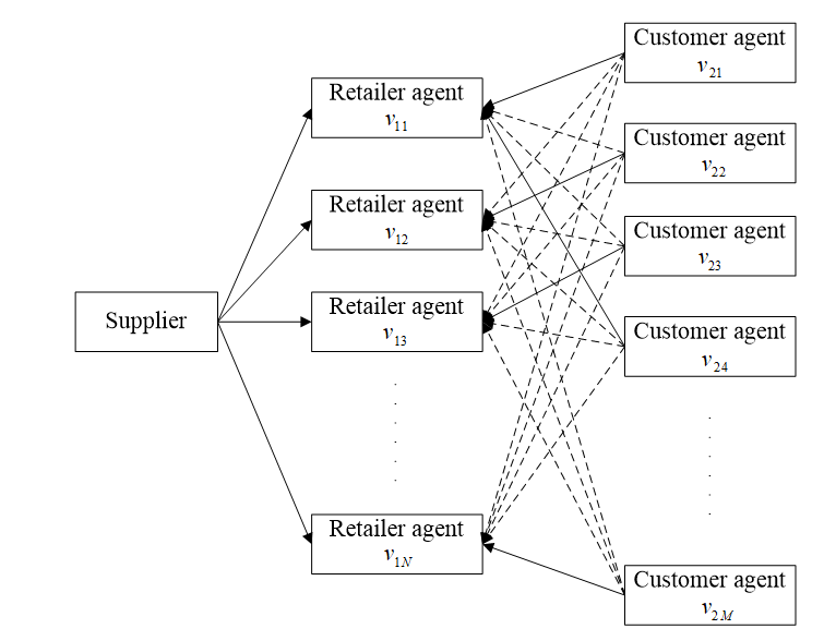
The competitive market consists of several competitive members (retailers) who compete for customers. Each member of the market (retailer and customer) is simulated by an agent in Netlogo 5.1.0. The virtual competitive market \(G\) (\(G = \langle V_1, V_2, E \rangle\)) consists of \(N\) retailer agents (\(V_1 = \{ v_{11}, v_{12}, v_{13}, \dots, v_{1N} \}\) and \(M\) customer agents (\(V_2 = \{ v_{21}, v_{22}, v_{23}, \dots, v_{2M} \}\). The relationship between retailers and customers is modeled by an adjacency matrix \(E\). \(e_{ij}^t\) is the element of the adjacency matrix \(E\). The relationships among suppliers, retailers and customers are shown in Figure 1, in which a solid arrow means \(e_{}ij = 1\), while a dotted arrow means \(e_{}ij = 0\). \(e_{ij}\) should satisfy the following constraint:
| $$\sum_{j = 1}^N e_{ij} = 1 \text{,} \quad \forall i \in M$$ | (1) |
The state of retailer agents
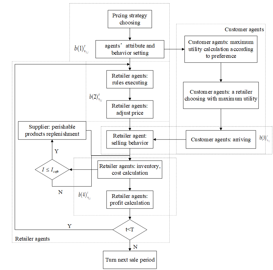
The state of \(v_{1j}\) is defined as \(S_{v_{1j}}^t = \bigl\{ f_{v_{1j}}^t, f_{I_{1j}}^t, x_{v_{1j}}^t, B_{v_{1j}}^t \bigr\}\). \(B_{v_{1j}}^t = \bigl\{ b(1)_{v_{1j}}^t, b(2)_{I_{1j}}^t, b(3)_{v_{1j}}^t, b(4)_{v_{1j}}^t \bigr\}\), where \(b(1)_{v_{1j}}^t\) is the price strategy that agent \(v_{1j}\) chooses at time \(t\), \(b(2)_{v_{1j}}^t\) is the action of \(v_{1j}\) used to adjust his price at time \(t\), \(b(3)_{v_{1j}}^t\) means the selling action of \(v_{1j}\) at time \(t\), and \(b(4)_{v_{1j}}^t\) is the action used to calculate costs, profit and inventory at time \(t\). Figure 2 shows the dynamic processes of retailer agents. If the inventory of agent \(v_{1j}\) at time \(t\) is \(I_{v_{1j}}^t - (D_{v_{1j}}^t + (I_{v_{1j}}^t + I_{v_{1j}}^t - D_{v_{1j}}^t) \times \psi ) < 0\), then \(FO_{v_{1j}}^t = 1\) (Chen et al. 2016); otherwise \(FO_{v_{1j}}^t = 0\). When \(FO_{v_{1j}}^t = 1\), the retailer agent orders Q perishable products from a supplier, otherwise it issues no orders. The order policy is the same for each retailer agent. \(f_{v_{1j}}^t\) can be calculated as follows:
| $$f_{v_{1j}}^t = f_{v_{1j}}^{initial} + \sum_t f_{v_{1j}, t}^{profit} $$ | (2) |
\(f_{v_{1j}, t}^{profit} = f_{v_{1j}, t}^{income} - f_{v_{1j}, t}^{cost}\). \(f_{v_{1j}, t}^{cost}\) is calculated by Equation 3 (Chen et al. 2016):
| $$f_{v_{1j}, t}^{cost} = \Bigl( \frac{C_1}{Q} + C_2 + C_3 \Bigr) \Bigl( D_{v_{1j}}^t + \bigl( I_{v_{1j}}^t + \bigl( I_{v_{1j}}^t - D_{v_{1j}}^t \bigr) \bigr) \times \psi \Bigr)$$ | (3) |
\(f_{v_{1j}, t}^{income}\) is calculated by \(f_{v_{1j}, t}^{income} = x_{v_{1j}}^t \times D_{v_{1j}}^t\), while \(D_{v_{1j}}^t\) is calculated by Function 4:
| $$D_{v_{1j}}^t = \sum_i^M e_{ij}^t D_{v_{2i}}$$ | (4) |
| $$D_{v_{1j}}^t = \begin{cases} D_{v_{1j}}^t \text{,} & I_{v_{1j}}^t - \bigl( I_{v_{1j}}^t + I_{v_{1j}}^t - D_{v_{1j}}^t \bigr) \times \psi - D_{v_{1j}}^t \geq 0 \\ I_{v_{1j}}^t - \frac{I_{v_{1j}}^t}{2} \times \psi \text{,} & \text{otherwise} \end{cases} $$ | (5) |
| $$I_{v_{1j}}^t = \begin{cases} I_{v_{1j}}^{t - 1} - \bigl( I_{v_{1j}}^{t - 1} + I_{v_{1j}}^{t - 1} - D_{v_{1j}}^t \bigr) \times \psi - D_{v_{1j}}^{t - 1} \text{,} & I_{v_{1j}}^{t - 1} - \bigl( I_{v_{1j}}^{t - 1} + I_{v_{1j}}^{t - 1} - D_{v_{1j}}^t \bigr) \times \psi - D_{v_{1j}}^t \geq 0 \\ Q \text{,} & \text{otherwise} \end{cases} $$ | (6) |
Equation 5 means that the retailer’s demand is determined by its inventory at the \(t\)th cycle. If the inventory is less than customer demand, only part of the overall customer demand will be satisfied (\(D_{v_{1j}}^t = I_{v_{1j}}^t - \frac{I_{v_{1j}}^t}{2} \times \psi\)). Similar to \(D_{v_{ij}}^t\), the value of \(I_{v_{ij}}^t\) is determined by its inventory at the \((t-1)\)th cycle. If the final inventory of retailer agent \(v_{1j}\) at the \((t-1)\)th cycle is less than zero, an order will be generated, and the inventory at the \(t\)th cycle will equal \(Q\). Equation 6 shows this type of relationship. The initial stocks of all retailers are assumed to be the same (Chang et al. 2016), as Equation 7 shows.
| $$\forall j \text{,} \quad I_{v_{1j}}^0 = Q$$ | (7) |
In these models, shortages are allowed but cannot be backlogged. Moreover, the value deterioration rate of perishable products should be considered. Different types of perishable products have different rates of deterioration based on their characteristics. Blackburn & Scudder (2009) and Chang et al. (2016) described the diminishing value of perishable products at time t in the form of an exponential function, as shown in Equation 8. They all assumed that perishable goods with the same criteria have similar qualities.
| $$r (t) = e^{-\alpha t}$$ | (8) |
\(0 < \alpha < 1\), \(t > 0\), \(0 \leq r (t) \leq 1\). When \(t\), \(r (t) = 1\) perishable products are completely fresh; When \(\lim_{t \to \infty} r (t) = 0\), the perishable products are useless. If \(r (t) < \xi\), set \(FO_{v_{ij}}^t = 1\). \(V\) is the customer acceptable value coefficient.
State of customer agents
The state of customer agents can be described as \(S_{v_{2i}}^t = \bigl\{ D_{v_{2i}}, e_{ij}^t, \delta_{v_{2i}} \bigr\}\). The demand of each customer follows a normal distribution \(D_{v_{2i}} \sim N (u, \sigma^2)\). It is assumed that each customer’s requirement is independent of the retailer’s pricing policy. \(e_{ij}^t\) is a 0-1variable, which is used to describe the retailer choosing the actions of customer agents. The actions of a retailer choosing for all customer agents at time \(t\) can be described via adjacency matrix \(E\) that is shown by Equation 9.
| $$E = \begin{vmatrix} e_{11}^t & e_{21}^t & \dots & e_{(M - 1) 1}^t & e_{M1}^t \\ e_{12}^t & e_{22}^t & \dots & e_{(M - 1) 2}^t & e_{M2}^t \\ \vdots & \vdots & \ddots & \vdots & \vdots \\ e_{1(N - 1)}^t & e_{2 (N - 1)}^t & \dots & e_{(M - 1) (N - 1)}^t & e_{M(N-1)}^t \\ e_{1N}^t & e_{2N}^t & \dots & e_{(M - 1) N}^t & e_{MN}^t \\ \end{vmatrix} $$ | (9) |
In matrix \(E\), each column should satisfy the Equation 1. \(\delta_{v_{2i}}\) represents customer preferences that are affected by age, regional culture and personal factors (such as life habits and personality) (Feldmann & Hamm 2015; Chang et al. 2016). \(\delta_{v_{2i}} = \{\delta (1)_{v_{2i}}, \delta (2)_{v_{2i}} \}\). \(\delta (1)_{v_{2i}}\) is a \(K \times N\) set, in which each element is one preference type (\(\delta (1)_{v_{2i}} = \{ s_{1i1}, s_{1i2}, \dots, s_{1iN}, s_{2i1}, s_{2i2}, \dots, s_{2iN}, \dots, s_{KiN} \}\)). The proportion of each preference is defined as set \(\delta (2)_{v_{2i}}\) (\(\delta (2)_{v_{2i}} = \{ \gamma_{1i}, \gamma_{2i}, \gamma_{3i}, \dots, \gamma_{Ki} \}\)), and \(\sum_{k = 1}^K \gamma_{ki} = 1\). Customer agents’ actions are shown in Figure 2. In this paper, two kinds of preferences are considered. The first preference is the distance between customer and retailer. It can determine the convenience of consumption (Chang et al. 2016). Price is another customer preference. Compared to quality-oriented customers, this kind of customer is sensitive to price (Lee et al. 2014). Based on this, customers can be divided into three categories (See Table 2). For example, customer 2 prefers a retailer with a lower price. The retailer choosing processes can be described as follows:
Step 1: For each \(k\), calculate the value \(s_{ki1}, s_{ki2}, s_{ki3}, \dots, s_{kin}\) of customer agents \(\delta_{v_{2i}}\) (\(k\) means the \(k\)th preference of customers).
Step 2: For each \(k\), set \(s_{ki} = s_{ki1}, s_{ki2}, s_{ki3}, \dots, s_{kin}\), \(\forall k \leq 2\).
Step 3: Normalize the \(k\)th preference value of customer agent \(\delta_{v_{2i}}\), \(y_{kij} = \frac{s_{kij} - \min \{ s_{ki} \} }{\max \{ s_{ki} \} - \min \{ s_{ki} \} } \) (according to the synthesizing evaluation function of customer preferences). \(y_{kij}\) is the normalized \(k\)th preference value from customer agent \(v_{2i}\) to retailer agent \(v_{ij}\), \(y_{kij} \in [0,1]\).
Step 4: For each retailer agent \(v_{1j}\), calculate the total preference value \(\delta '\) of customer agent \(v_{2i}\), \(\delta ' = \sum_{k = 1}^2 ( \gamma_{ki} \times y_{kij}\)). The customer agent \(v_{2i}\) chooses the retailer agent with the maximum \(\delta '\).
| Customer categories | Distance | Price |
| Customer 1 | Sensitive | Insensitive |
| Customer 2 | Insensitive | Sensitive |
| Customer 3 | Equal | Equal |
Q-learning algorithm for dynamic pricing policy
The dynamic pricing process of \(X_{v_{1j}}\) is the Markov decision process (MDP), given the transition function:
| $$T ( x_{v_{1j}}^t, a_{v_{1j}}^t, x_{v_{1j}}^{t + 1} ) = P \bigl( X_{v_{1j}}^{t + 1} = x_{v_{1j}}^{t + 1} | X_{v_{1j}}^t = x_{v_{1j}}^t, \, A_{v_{1j}}^t = a_{v_{1j}}^t \bigr) $$ | (10) |
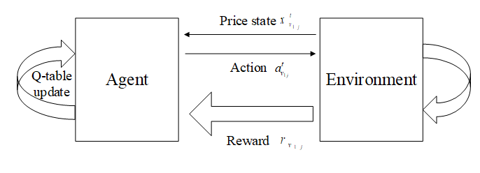
Q-learning reward function
The Q-learning algorithm can be viewed as a sampled, asynchronous method for estimating the optimal Q-function of the MDP (\(\bigl\{ X_{v_{1j}}, A_{v_{1j}}, T_{v_{1j}}, R_{v_{1j}} \bigr\}\)). The reward \(r_{v_{1j}}^t\) at period \(t\) is determined by customer demand, product price and retailer total cost. All customer demand can be described by the set \(D^t = \bigl\{ D_{v_{21}}^t, D_{v_{22}}^t, \dots D_{v_{2M}}^t \bigr\}\). The customer decision matrix is \(E^t_{v_{1j}}\). Then, the reward function can be calculated by:
| $$r_{v_{1j}}^t = \Bigl(f_{v_{1j}, t}^{income} - f_{v_{1j}, t}^{cost} \Bigr) - \Bigl(f_{v_{1j}, t - 1}^{income} - f_{v_{1j}, t - 1}^{cost} \Bigr) = \Bigl( \sum_{i = 1}^M D_{v_{1j}}^t e_{ij}^t x_{v_{1j}}^t - f_{v_{1j}, t}^{cost} \Bigr) - \Bigl( \sum_{i = 1}^M D_{v_{1j}}^{t - 1} e_{ij}^{t-1} x_{v_{1j}}^{t-1} - f_{v_{1j}, t-1}^{cost} \Bigr) $$ | (11) |
Q-learning action
The Q-function \(Q( x_{v_{1j}}, x_{a_{1j}} )\) defines the expected sum of the discounted reward attained by executing action \(a_{v_{1j}}\) (\(a_{v_{1j}} \in A_{v_{1j}}\)) in state \(x_{v_{1j}}\) (\(x_{v_{1j}} \in X\)). The Q-function is updated by using the agent’s experience. The learning process is as described below.
Agents observe the current state and select an action from \(A_{v_{1j}}\). Boltzmann soft-max distribution is adopted to select the actions. For each price state, \(A_{v_{1j}} = \{ a_{v_{1j}}^0, a_{v_{1j}}^1, a_{v_{1j}}^2 \}\), where \(a_{v_{1j}}^0\) means a price decrease, \(a_{v_{1j}}^1\) means on operation occurs to the price and \(a_{v_{1j}}^2\) means a price increase. The probability calculation of action is similar to that described by Li et al. (2011).
\(e_u\): The tendency of agents to explore unknown actions.
\(A_u\): The set of unexplored actions from the current state.
\(A_w\): The set of explored actions (at least once) from the current state.
The probability of \(P \bigl( a_{v_{1j}}^m | x_{v_{1j}} \bigr)\) can be calculated by:
| $$P \bigl( a_{v_{1j}}^m | x_{v_{1j}} \bigr) = \frac{e^{Q( x, a_{v_{1j}}^m )}}{\sum_n e^{Q( x, a_{v_{1j}}^m )}} $$ | (12) |
If one of the actions belongs to \(A_w\) and the others belong to \(A_u\), then
| $$P \Bigl( a_{v_{1j}}^m | x_{v_{1j}} \Bigr) = \begin{cases} 1 - e_u & \text{for} \,\, a_{v_{1j}}^m \in A_w \\ \frac{e_u}{2}& \text{for} \,\, a_{v_{1j}}^m \in A_u \\ \end{cases} $$ | (13) |
If only one action belongs to \(A_u\), then
| $$P \Bigl( a_{v_{1j}}^m | x_{v_{1j}} \Bigr) = \begin{cases} \frac{(1 - e_u) e^{Q( x, a_{v_{1j}}^m )}}{\sum_n e^{Q( x, a_{v_{1j}}^m )}} & \text{for} \,\, a_{v_{1j}}^m \in A_w \\ e_u & \text{for} \,\, a_{v_{1j}}^m \in A_u \\ \end{cases} $$ | (14) |
After selecting an action, the agent observes the state at period \(t+1\) and receives a reward for the system. The corresponding Q value for state \(x_{v_{1j}}\) and action \(a_{v_{1j}}\) are updated according to the following formula:
| $$Q ( x_{v_{1j}}, a_{v_{1j}} ) = ( 1 - \epsilon ) Q ( x_{v_{1j}}, a_{v_{1j}} ) + \epsilon ( re ( x_{v_{1j}}, a_{v_{1j}} ) + \eta \max_{a' v_{1j}} Q ( x '_{v_{1j}}, a '_{v_{1j}})) $$ | (15) |
In order to prevent premature convergence, a random parameter is introduced to describe the step size (\(a^t_{v_{1j}, x^t_{v_{1j}}, -x_{v_{1j}}}\)) of price decreases or increases.
| $$a^t_{v_{1j}, x^t_{v_{1j}}, -x_{v_{1j}}} = \begin{cases} - random ( x_{v_{1j}} - x_{v_{1j}, lower} ) \text{,} & \text{if} a_{v_{1j}} = a_{v_{1j}}^0 \\ 0 & \text{if} a_{v_{1j}} = a_{v_{1j}}^1 \\ random ( x_{v_{1j}, upper} - x_{v_{1j}} ) & \text{if} a_{v_{1j}} = a_{v_{1j}}^2 \\ \end{cases} $$ | (16) |
where \(x_{v_{1j}, lower}\) and \(x_{v_{1j}, upper}\) denote the upper and lower price limits of retailer agent \(v_{1j}\), and \(x '_{v_{1j} = a^t_{v_{1j}, x'_{v_{1j}} - x_{v_{1j}}} + x_{v_{1j}}}\). Equation 16 is a piecewise function, and its meaning can be described as follows:
- If a retailer agent with the Q-learning algorithm chooses the action to decrease a price, the decreased step size should be a random value between \([0, ( x_{v_{1j}} - x_{v_{1j}, lower} )]\);
- If a retailer agent with the Q-learning algorithm chooses the action to increase a price, the increased step size should be a random value between \([0, ( x_{v_{1j}, upper} - x_{v_{1j}} )]\);
- In any other situation, the step size should be zero.
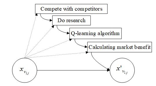
In this model, retailer agents adjust their price values based on market judgments. Figure 4 shows the basic graphical model of this paper. Dotted arrows indicate that an action is chosen depending on the state.
A complete learning process occurs from the initial state to the terminal state. This is considered one cycle. The Q-learning process is shown in Table 3. The Q-learning algorithm contains two steps: action determination based on the current Q-value and evaluation of a new action via the reward function. This cycle continues until the Q-value converges.
| Initialize \(Q(x_{v_{1j}}, a_{v_{1j}})\) arbitrarily, \(\pi\) to the policy to be evaluated Repeat (for each cycle) \(\quad\) Initialize \(x_{v_{1j}}\) \(\quad\) Repeat (for each step of cycle) \(\quad\) \(\quad\) Choose \(a_{v_{1j}}\) from \(x_{v_{1j}}\) using policy \(\pi\) derived from \(Q\) \(\quad\) \(\quad\) Take action \(a_{v_{1j}}\) \(\quad\) \(\quad\) Set \(x'_{v_{1j}} = x_{v_{1j}} + a_{v_{1j}, X' - x}\) \(\quad\) \(\quad\)Observe \(r_{v_{1j}}$, $x'_{v_{1j}}\) \(\quad\) \(\quad\) \(Q ( x_{v_{1j}}, a_{v_{1j}} ) = ( 1 - \epsilon ) Q ( x_{v_{1j}}, a_{v_{1j}} ) + \epsilon ( re ( x_{v_{1j}}, a_{v_{1j}} ) + \eta \max_{a' v_{1j}} Q ( x '_{v_{1j}}, a '_{v_{1j}})) x_{v_{1j}} \leftarrow x'_{v_{1j}}\) Until \(x_{v_{1j}}\) is terminal |
Other pricing policies
In real-market situations, there are many pricing policies. Three of these pricing policies are considered (Chang et al. 2016) and compared with the Q-learning algorithm proposed in this article.
- Cost-plus pricing strategy. A product’s price is set based on unit cost (ordering cost, inventory cost and other factors) with a degree of profit. Once the price is calculated, it remains constant throughout the entire sales cycle. \(x(t)\) is calculated by equation (17), where \(\lambda\) is the target profit coefficient.
| $$x_{v_{1j}} = \Biggl( \frac{C_1}{Q} + C_2 + C_3 \Biggr) \times ( 1 + \lambda ) $$ | (17) |
- Value-based pricing strategy. This pricing policy is suitable for customers with high product quality. The value of perishable product tends to decrease during the sales cycle, so the price becomes cheaper as time passes. The price calculation formula is shown in Equation 18 and Equation 19, where \(m\) and \(\beta\) are the freshness impact factors, \(\theta\) is the basic price for retailers and \(T\) is the theoretical sales cycle.
| $$x_{v_{12}} (t) = m \cdot e^{-\beta t} + \theta (\alpha > 0, \theta > 0, 0 < t < T) $$ | (18) |
| $$T = \frac{QN}{\sum_{i = 1}^M D_{v_{2i}}}$$ | (19) |
- Inventory-sensitive pricing strategy. A larger inventory will typically cause lower prices, so that the retailer may sell products more quickly and reduce outdating. The price can be calculated by equation (20), where \(I_{cu}\) is current inventory, \(x_{13}\) is the basic price for retailers, \(x_{min}\) and \(x_{max}\) mean the upper and lower prices respectively, and \(f_{in}\) is the inventory-price coefficient. Standard inventory \(I_{st}\) is equal to \(I_{st} = \Bigl( 1 - \frac{t}{T} \Bigr) \cdot Q\).
| $$x_{v_{13}}(t) = \begin{cases} x_{min}\text{,} & f_{in} \Bigl( 1 - \frac{I}{I_st} \Bigr) < 0 \\ x_{v_{13}} + f_{in} \Bigl( 1 - \frac{I}{I_st} \Bigr) \text{,} & 0 \leq f_{in} \Bigl( 1 - \frac{I}{I_st} \Bigr) < x_{max} - x_{min} \\ x_{max} \text{,} & f_{in} \Bigl( 1 - \frac{I}{I_st} \Bigr) \geq x_{max} - x_{min} \end{cases} $$ | (20) |
Runs of the Model
A virtual market is established in the Netlogo platform. Different categories of retailers and customers can be distinguished by different colors. The general model parameters agree with the conditions of the Nanjing Jinxianghe (China) vegetable market. Market information was obtained from http://nw.nanjing.gov.cn/ (Chang et al. 2016) (shown in Appendix). This experiment also takes the selling of grape as an example. The price of grapes in the market is between 7 and 11 Yuan. To calculate a reasonable price of retailer agents, \(x_{v_{1j}, lower}\) is set to 6 Yuan and \(x_{v_{1j}, upper}\) is set to 12 Yuan. \(x_{min} = x_{v_{1j}, lower}\) and \(x_{max} = x_{v_{1j}, upper}\). There are four retailer agents and hundreds of customer agents. Customer demand is assumed to be normal, distributed according to \(D_{v_{2i}} \sim N(3,1)\). To balance freshness and the ordering frequency, the threshold quantity for restocking perishable products is set to 800kg. Other parameters are set based on previous research (Chang et al. 2016; Li et al. 2011).
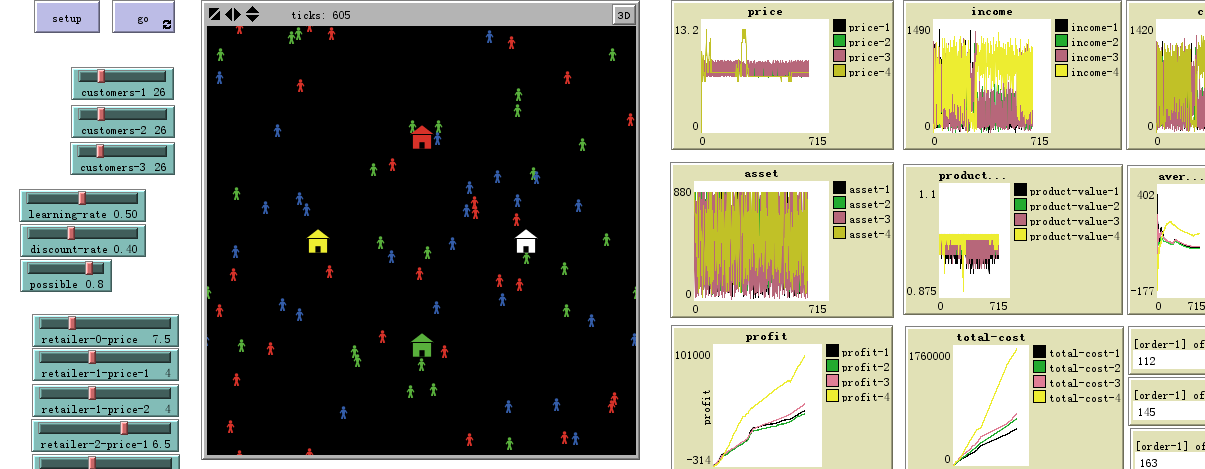
Four scenarios are run for this dynamic price competitive market to quantify the performance of the dynamic pricing strategies. The four experiments are (i) sensitivity experiments on the learning rate and discount rate, (ii) sensitivity experiments on customer demand, (iii) sensitivity experiments on customer preferences, and (iv) sensitivity experiments on retailer pricing behavior. In these scenarios, a retailer agent with the Q-learning algorithm chooses the optimal action to maximize the sums of its fitness. The results of these experiments are shown in Sections 4.1-4.7. The parametric settings for the experiments are presented in Table 5. The values of several parameters refer to Chang et al. (2016). These parameters are efficient to verify the effectiveness of the simulation model. Other market can utilize the model as well. The Netlogo interface of the competitive market is proposed in Figure 5. In the simulation, retailer agent \(v_{11}\) runs with the Cost-Plus Pricing Strategy, retailer \(v_{12}\) runs with the Value-Based Pricing Strategy, retailer \(v_{13}\) runs with the Inventory-Sensitive Pricing Strategy, and retailer \(v_{14}\) runs with the Q-learning algorithm. The quantity of different kinds of customer agents is changed according to the different situations.
| Parameter | Value |
| Preference | (0.8,0.2); (0.2,0.8); (0.5,0.5) |
| \(j\) | 4 |
| \(D_{v_{2i}}\) | N(3,1) |
| \(\psi\) | 0.005 |
| \(c_1\) | 200 |
| \(c_2\) | 5.5 |
| \(c_3\) | 0.4 |
| Q | 800 |
| \([ x_{v_{1j}, lower}, x_{v_{1j}, upper} ]\) | [6,12] |
| \(\alpha\) | 0.01 |
| \(\beta\) | 0.1 |
| \(f_{in}\) | 2 |
| \(e_u\) | 0.8 |
| \(x_{v_{11}}\) | 7.5 |
| \(m\) | 4 |
| \(\theta\) | 4 |
| \(x_{v_{13}}\) | 6.5 |
| \(\epsilon\) | 0.5 |
| \(\eta\) | 0.4 |
Simulation results
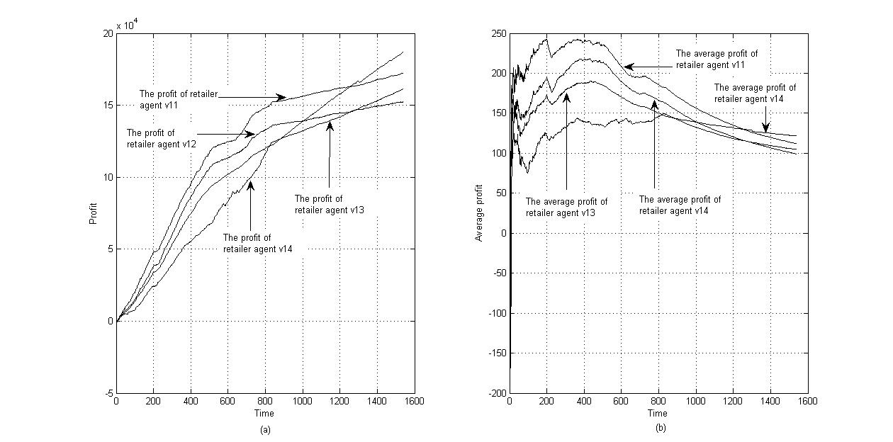
Take a set of parameters arbitrarily, e.g. \(x_{v_{11}} = 7.5\), \(m = 4\), \(\theta = 4\), \(x_{v_{13}} = 6.5\), \(\epsilon = 0.5\), \(\eta = 0.4\), based on market information from Nanjing, China. These parameters can maintain the average price of retailer agents in the same level, and it can eliminate the positive effect of optimal strategy choosing. The position of customer agents is set randomly. The quantities of customer 1, customer 2 and customer 3 are assumed to be 26. In this situation, the effectiveness of the Q-learning algorithm is verified by comparing the profits that the retailer agents gain. Figures 6 and 7 show the competitive results of the four retailer agents. Figure 6 shows the price aggregated trends of four retailer agents. It shows that the prices of retailer 2 and retailer 3 fluctuate between [6.5, 8], while the price of retailer 4 converges to 6.5. The learning effect of retailer 4 is more conclusive. Figure 7 shows the total profit and the average profit of the four retailer agents. During the initial stage, the total profit and the average profit of four retailer agents are all below zero, because \(f_{v_{1j}, t}^{income} - f_{v_{1j}, t}^{cost} < 0\). Then, the profit of the four retailer agents increases with the increase in trading volume, but the fluctuation of the marginal revenue is severe. The Q-learning algorithm performs better after 1200 steps, and the price war tends to stabilize after 1400 steps.

Sensitivity experiments
In this section, we estimate the optimal pricing strategy for retailers considering various market conditions. The economic behavior of customer agents and retailer agents is observed. The experiments simulate four scenarios. The sensitivity results from these experiments are shown in Sections 4.4-4.7.
Sensitivity experiments on the learning and discount rates
This section conducts two sets of sensitivity experiments with respect to learning rate \(\epsilon\) and discount rate \(\eta\). The parameters are set as Table 5 shows. The quantities of customer 1, customer 2 and customer 3 are assumed to be 40. Other parameters are set as \(x_{v_{1j}} = 7.5\), \(m = 4\), \(\theta = 4\), \(x_{v_{3j}} = 6.5\). Wide parameter ranges are chosen to obtain the sensitive analysis. This section changes one parameter at a time, keeping the rest at their values, as shown in Table 3. If \(\epsilon\) is a variable, then set \(\eta = 0.4\). If \(\eta\) is a variable, then set \(\epsilon = 0.5\). For each parameter, the experiment is simulated over 2400 periods. Figure 8 shows the average profit of the four retailer agents with different discount and learning rates. The results suggest that the profits of retailer agents are sensitive to \(\eta\) (see Figure 8(a)) and \(\epsilon\) (see Figure 8(b)). The dynamic pricing strategy using the Q-learning algorithm can help retailers maintain a competitive edge except when \(\eta = 0.9\). The second-best pricing strategy is the inventory-sensitive pricing strategy. The fixed pricing strategy and the value-based pricing strategy result in a lack of competitive advantage in this kind of market. Moreover, the discount rate of the Q-learning algorithm reduces the intensity of competition in the market (the total profit of retailer agents increases), while the learning rate is the opposite. This is an interesting phenomenon, and it means that the retailer agent with a learning mechanism can lead market competition.
| Parameter | Minimum | Maximum | Sensitivity step |
| \(\epsilon\) | 0.1 | 0.9 | 0.2 |
| \(\eta\) | 0.1 | 0.9 | 0.2 |

Sensitivity experiments on market demand
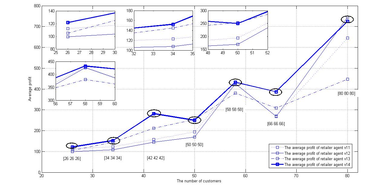
This section conducts a sensitivity analysis of market demand influence to observe how retailer agents share market returns with different dynamic pricing strategies. The market demand is mainly affected by the number of customers. In this scenario, the parameters are set as \(x_{v_{1j}} = 7.5\), \(m = 4\), \(\theta = 4\), \(x_{v_{3j}} = 6.5\), \(\epsilon = 0.5\), \(\eta = 0.4\). The variables are the quantities of different customer categories. For easy comparison, seven occasions in Table 6 are considered. Figure 9shows the average profit of retailer agents, and it describes the competition results clearly. Retailer agents with Q-learning maintain a competitive advantage, while other dynamic pricing strategies only work well in certain situations. For example, the inventory-sensitive pricing strategy win the competition in occasion 4. However, behaves poorly in occasion 5. Interestingly, the total profit of all retailer agents increased with customer demand, except for in occasion 6. In this occasion, the underpricing behaviors of retailer agents \(v_{12}\) and \(v_{13}\) disordered the market.
| Occasion | Customer 1 | Customer 2 | Customer 3 |
| 1 | 26 | 26 | 26 |
| 2 | 34 | 34 | 34 |
| 3 | 42 | 42 | 42 |
| 4 | 50 | 50 | 50 |
| 5 | 58 | 58 | 58 |
| 6 | 66 | 66 | 66 |
| 7 | 80 | 80 | 80> |
Sensitivity experiments on customer preference
This section conducts a sensitivity analysis of customers’ preferences to observe how customer behavior affects the profit of retailer agents, as in Table 7 and Table 8. The parameters are set as \(x_{v_{1j}} = 7.5\), \(m = 4\), \(\theta = 4\), \(x_{v_{3j}} = 6.5\), \(\epsilon = 0.5\), \(\eta = 0.4\), and the number of all kinds of customers is set at 40. First, the preference of the first kind of customer is considered (occasion 1). The variable is the customer preference degree for price and distance. Table 7 is the sensitivity results, and it shows the average profit of the four retailer agents considered in this situation. The results reveal that the dynamic pricing strategy with the Q-learning algorithm performs well no matter how much customers’ preferences change. Interestingly, the insensitivity to price of the first kind of customer can reduce competition among retailer agents. Retailer agents share more market revenue in this occasion. Then, the preference of the second kind of customer is considered (occasion 2). The sensitivity results are shown in Table 8. In this situation, the dynamic pricing strategy proposed in this paper has a clear competitive edge as well. However, there is no obvious relationship between customer preference and market revenue.
| Retailer agent | \(\mathbf{\delta (2)_{v_{2,1}}} \sim\) | \(\mathbf{\delta (2)_{v_{2,40}}}\) | |||
| [0.6, 0.4] | [0.7, 0.3] | [0.8, 0.1] | [0.9, 0.1] | ||
| \(v_{11}\) | 113.4 | 150.9 | 232.7 | 303.6 | [0.2, 0.8] \(\delta(2)_{v_{2,41}} \sim \delta(2)_{v_{2,80}}\) |
| \(v_{12}\) | 102.9 | 137.2 | 225.9 | 286.1 | |
| \(v_{13}\) | 138.6 | 175.5 | 230.4 | 296.9 | |
| \(v_{14}\) | 195.3 | 197.3 | 253.4 | 317.5 |
| Retailer agent | \(\mathbf{\delta (2)_{v_{2,41}}} \sim\) | \(\mathbf{\delta (2)_{v_{2,80}}}\) | |||
| [0.6, 0.4] | [0.7, 0.3] | [0.8, 0.1] | [0.9, 0.1] | ||
| \(v_{11}\) | 123.6 | 232.7 | 139.8 | 149.7 | [0.8, 0.2] \(\delta(2)_{v_{2,1}} \sim \delta(2)_{v_{2,40}}\) |
| \(v_{12}\) | 110.5 | 225.9 | 113.5 | 139.6 | |
| \(v_{11}\) | 148.2 | 230.4 | 153.3 | 227.9 | |
| \(v_{11}\) | 217.6 | 254.4 | 178.2 | 268.4 |
Sensitivity experiments on retailer price
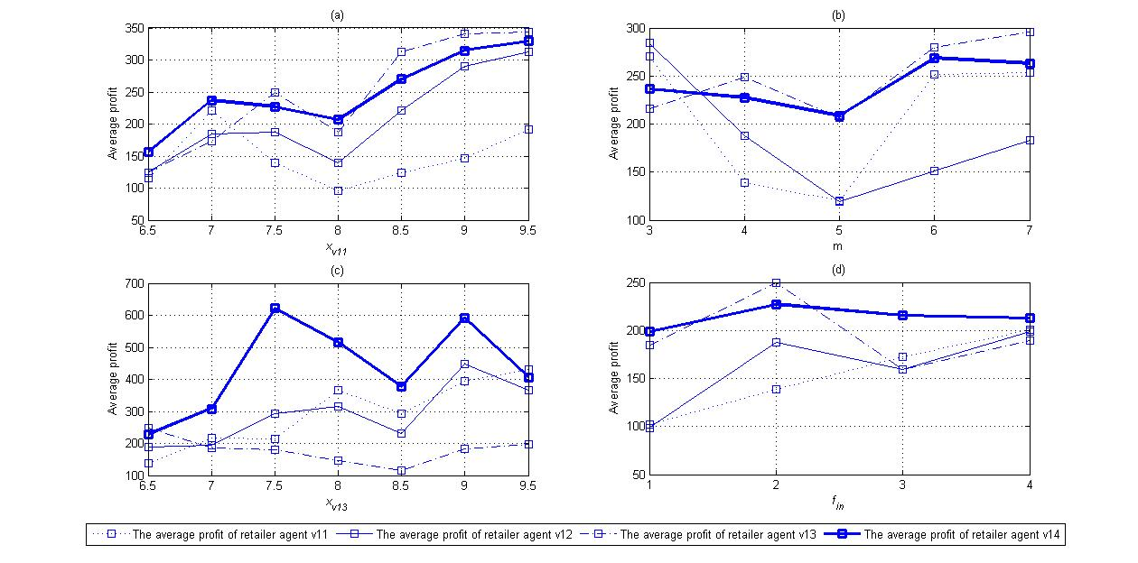
This section conducts a sensitivity analysis of retailer price to observe how retailers’ pricing behaviors affect the profit of the retailer agents. The number of customers is set to 40. There are four scenarios, and the sensitivity results are shown in Figure 10. The variables in the four scenarios are the fixed price of retailer agent \(v_{11}\), the freshness impact factor \(m\) of retailer agent \(v_{12}\), the basic price \(x_{v_{13}}\) and the inventory-sensitive coefficient \(f_{in}\) of retailer agent \(v_{13}\), respectively. The paper changes one parameter at a time, keeping the rest at the values shown in Table 3. Figure 10(a) is the average profit of retailer agents in scenario 1, Figure 10(b) is the average profit of retailer agents in scenario 2, Figure 10(c) is the average profit of retailer agents in scenario 3 and Figure 10(d) is the average profit of retailer agents in scenario 4. The profit of each retailer agent is sensitive to the price of the others. In scenarios 3 and 4, the dynamic pricing strategy with the Q-learning algorithm is superior to other pricing strategies. However, the competitive edge of this pricing strategy decreases in scenarios 1 and 2. The sensitivity results also reveal that a high pricing strategy does not always bring benefits to retailers in a perishable product market. Profits in this type of market depend on customer preference and the pricing strategies of other retailers.
Conclusions
Retailers with perishable products struggle in a competitive market environment. This paper researches the pricing strategies of retailers with perishable products, taking into account customer preferences. First, how agent-based modeling helps to inform pricing strategies in a competitive environment is demonstrated. The trade behaviors between retailers and customers are simulated in the model. Traditional retailers in the market adopt pricing strategies based on product freshness, inventory, cost and other factors. Customers in the market have different preferences of price and distance from certain retailers. Second, this paper presents a dynamic pricing model, using the Q-learning algorithm, to solve pricing problems in a virtual competitive market. The algorithm allows retailer agents to adjust their price, informed by observations of their experience. The optimal pricing strategy is measured by the final profit in different situations.
The proposed simulation model was applied to the Nanjing Jinxianghe (China) vegetable market. Sensitivity experiments are shown to observe how certain factors, such as the learning rate and discount rate of Q-learning, customer demand, customer preferences and the basic price of retailers, affect pricing strategy. The optimal strategy is calculated under different market conditions. According to our findings, the Q-learning algorithm can be used as an effective dynamic price approach in most competitive conditions. However, this strategy is not always optimal in every market. If a retailer adjusts its basic price parameter, the competitive environment changes, and so does the optimal pricing strategy. For example, an inventory-sensitive pricing strategy may produce higher profits when retailer agent \(v_{11}\) adjusts its fixed price or retailer agent \(v_{12}\) adjusts its freshness impact factor.
The proposed simulation should be suitable for a wide range of market conditions and may be implemented by adjusting the parameters in the model. It is beneficial to research the pricing problem of perishable products, and our work can be extended along several directions. For example, retailers in markets may have various perishable products to sell, and the products may influence each other. In future research, a more complex learning mechanism should be constructed to improve the retailer agents’ learning ability. These are the key issues for future research of perishable products’ dynamic price strategies.
Acknowledgements
This research was supported in part by: MSSFC (Major Social Science Foundation of China) program under Grant 15ZDB151; SSFC (Social Science Foundation of China) program under Grant 16BGL001.Appendix: The market information from Nanjing, China
The price information of grape in Nanjing, China are shown in Figures 11 and 12. Figure 11 is the price of grapes in July, 2016. Figure 12 is the price of grapes in August, 2016. The two Figures show that the normal price of grapes in the market is between 7 Yuan and 11 Yuan. All price parameters should be set based on the market information.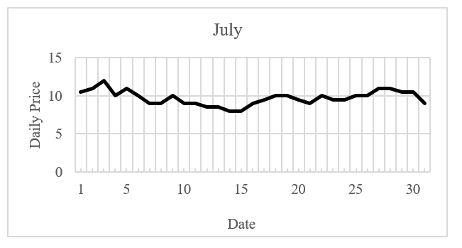

References
ADENSO-DÍAZ, B., Lozano, S., & Palacio, A. (2017). Effects of dynamic pricing of perishable products on revenue and waste. Applied Mathematical Modelling, 45, 148-164. [doi:10.1016/j.apm.2016.12.024]
AKCHURINA, N. (2008). Optimistic-pessimistic Q-learning algorithm for multi-agent systems. In R. Bergmann, G. Lindemann, S. Kirn & M. Pěchouček (Eds.), Multiagent System Technologies: 6th German Conference, MATES 2008. Kaiserslautern, Germany, September 23–26, 2008. Proceedings, (pp. 13-24). Berlin/Heidelberg: Springer.
ARSLAN, I., Caverzasi, E., Gallegati, M., & Duman, A. (2016). Long term impacts of bank behavior on financial stability: an agent based modeling approach. Journal of Artifical Societies and Social Simulation, 19(1), 11: https://www.jasss.org/19/1/11.html.
BLACKBURN, J., & Scudder, G. (2009). Supply chain strategies for perishable products: the case of fresh produce. Production and Operations Management, 18(2), 129-137.
CHANG, X., Li, J., Rodriguez, D., & Su, Q. (2016). Agent-based simulation of pricing strategy for agri-products considering customer preference. International Journal of Production Research, 54(13), 3777-3795. [doi:10.1080/00207543.2015.1120901]
CHEN, W, Li, J., & Jin, X.J. (2016). The replenishment policy of agri-products with stochastic demand in integrated agricultural supply chains. Expert Systems with Applications, 48, 55-66.
CHUNG, J., & Li, D. (2013). The prospective impact of a multi-period pricing strategy on consumer perceptions for perishable foods. British Food Journal, 115(3), 377-393. [doi:10.1108/00070701311314200]
CHUNG, J., & Li, D. (2014). A simulation of the impacts of dynamic price management for perishable foods on retailer performance in the presence of need-driven purchasing consumers. Journal of the Operational Research Society, 65(8), 1177-1188.
COLLINS, A., & Thomas, L. (2012). Comparing reinforcement learning approaches for solving game theoretic models: a dynamic airline pricing game example. Journal of the Operational Research Society, 63(8), 1165-1173. [doi:10.1057/jors.2011.94]
DOGAN, I., & Guner, A.R. (2015). A reinforcement learning approach to competitive ordering and pricing problem. Expert Systems, 32(1), 39-48.
DOS SANTOS, J.P.Q., de Melo, J.D., Neto, A.D.D., & Aloise, D. (2014). Reactive search strategies using reinforcement learning, local search algorithm and variable neighborhood search. Expert Systems with Applications, 41, 4939-4949. [doi:10.1016/j.eswa.2014.01.040]
ELMAGHRABY, W., & Keskinocak, P. (2003). Dynamic pricing in the presence of inventory considerations: research overview, current practices, and future directions. Management Science, 49(10), 1287-1309.
EVEN-DAR, E., & Mansour, Y. (2003). Learning rates for Q-learning. Journal of Machine Learning Research, 5, 1-25.
FELDMANN, C., & Hamm, U. (2015). Consumers’ perceptions and preferences for local food: A review. Food Quality & Preference, 40, 152-164.
GONG, X.T., Chao, X.L., & Zheng, S.H. (2014). Dynamic pricing and inventory management with dual suppliers of different lead times and disruption risks. Production and Operations Management, 23(12), 2058-2074. [doi:10.1111/poms.12221]
GUMUS, M., Ray, S., & Gurnani, H. (2012). Supply-side story: risks, guarantees, competition, and information asymmetry. Management Science, 58(9), 1694-1714.
IBRAHIM, M.N., & Atiya, A.F. (2016). Analytical solutions to the dynamic pricing problem for time-normalized revenue. European Journal of Operational Research, 254(2), 632-643. [doi:10.1016/j.ejor.2016.04.012]
JIANG, C., & Sheng, Z. (2009). Case-based reinforcement learning for dynamic inventory control in a multi-agent supply-chain system. Expert Systems with Applications, 36, 6520-6526.
KIM, S., Lee, K., Cho, J. K., & Kim, C.O. (2011). Agent-based diffusion model for an automobile market with fuzzy TOPSIS-based product adoption process. Expert Systems with Applications, 38(6), 7270-7276. [doi:10.1016/j.eswa.2010.12.024]
KWON, I.H., Kim, C.O., Jun, J., & Lee, J.H. (2008). Case-based myopic reinforcement learning for satisfying target service level in supply chain. Expert Systems with applications, 359(1-2), 389-397.
LEE, K., Lee, H., & Kim, C.O. (2014). Pricing and timing strategies for new product using agent-based simulation of behavioral consumers. Journal of Artificial Societies and Social Simulation, 17(2): 1: https://www.jasss.org/17/2/1.html.
LI, G., Xiong, Z.K., & Nie, J.J. (2009). Dynamic pricing for perishable products with inventory and price sensitive demand. Journal of Systems & Management, 18(4), 402-409.
LI, J., Sheng, Z.H., & Ng, K.C. (2011). Multi-goal Q-learning of cooperative teams. Expert Systems with Applications, 38(3), 1565-1574. [doi:10.1016/j.eswa.2010.07.071]
LI, X., Wang, J., & Sawhney, R. (2012a). Reinforcement learning for joint pricing, lead-time and scheduling decision in make-to-order systems. European Journal of Operational Research, 221(1), 99-109.
LI, Y., Cheang, B., & Lim, A. (2012b). Grocery Perishables Management. Production & Operations Management, 21(3), 504–517. [doi:10.1111/j.1937-5956.2011.01288.x]
MACDONALD, L., & Rasmussen, H. (2010). Revenue management with dynamic pricing and advertising. Journal of Revenue Pricing Management, 9(1-2), 126-136.
OLIVEIRA, F.S. (2014). Reinforcement learning for business modeling. In Encyclopedia of business analytics and optimization (pp. 2010-2019). IGI Global. [doi:10.4018/978-1-4666-5202-6.ch181]
RANA, R., & Oliveira, F.S. (2014). Real-time dynamic pricing in a non-stationary environment using model-free reinforcement learning. Omega-International Journal of Management Science, 47(9), 116-126.
RANA, R., & Oliveira, F.S. (2015). Dynamic pricing policies for interdependent perishable products or services using reinforcement learning. Expert Systems with Application, 42(1), 426-436. [doi:10.1016/j.eswa.2014.07.007]
REZA, M., & Behrooz, K. (2014). Optimizing the pricing and replenishment policy for non-instantaneous deteriorating items with stochastic demand and promotional efforts. Computers & Operations Research, 51, 302-312.
SCHWEPPE, F.C., Caramanis, M.C., & Tabors, R. (1985). Evaluation of spot price based electricity rates. IEEE Transaction on Power Apparatus Systems, 104(7), 1644-1655. [doi:10.1109/TPAS.1985.319194]
SHANKAR, V., & Bolton, R. (2004). An empirical analysis of determinations of retailer pricing strategy. Marketing Science, 23(1), 28-49.
SONI, H.N., & Patel, K.A. (2012). Optimal pricing and inventory policies for non-instantaneous deteriorating items with permissible delay in payment: fuzzy expected value model. International Journal of Industrial Engineering Computations, 3(3), 281-300. [doi:10.5267/j.ijiec.2012.02.005]
SUNG, N.H., & Lee, J.K. (2000). Knowledge assisted dynamic pricing for large-scale retailers. Decision Support Systems, 28(4), 347-363.
TESAURO, G., & Kephart, J.O. (2002). Pricing in agent economics using multi-agent Q-learning. Autonomous Agents and Multi-Agent Systems, 5(3), 289-304. [doi:10.1023/A:1015504423309]
TSAO, Y.C., & Sheen, G.J. (2008). Dynamic pricing, promotion and replenishment policies for a deteriorating item under permissible delay payments. Computers & Operations Research, 35(11), 3562-3580.
WEN, X.Q., Xu, C., Hu, Q.Y. (2016). Dynamic capacity management with uncertain demand and dynamic price. International Journal of Production Economics, 175, 121-131. [doi:10.1016/j.ijpe.2016.02.011]
YOUSEFI, S., Moghaddam, M.P., & Majd, V.J. (2011). Optimal real time pricing in an agent-based retail market using a comprehensive demand response model. Energy, 36(9), 5716-5727.
YUSTA, J.M., Khodr, H.M., & Urdaneta, A.J. (2007). Optimal pricing of default customers in electrical distribution systems: effect behavior performance of demand response models. Electric Power Systems Research, 77(5-6), 548-558. [doi:10.1016/j.epsr.2006.05.001]
ZHAO, W., & Zheng, Y.S. (2000). Optimal dynamic pricing for perishable assets with non-homogeneous demand. Management Science, 46(3), 375-388.
ZHOU, X. (2015). Competition or cooperation: a simulation of the price strategy of ports. International Journal of Simulation Modelling, 14(3), 463-474. [doi:10.2507/IJSIMM14(3)8.303]