
Introduction
Jon Elster (1989) addresses a fundamental question for both moral philosophers and social scientists: "what is it that glues societies together and prevents them from disintegrating?" A short answer to this question is, according to Elster and many others, "social norms". A norm is social insofar as it is "(a) shared by other people and (b) partly sustained by the approval or disapproval of others" (ibid. p. 99). Indeed, in the absence of any norm of behavior that coordinates individual actions together, the tendency to maximize individual utility may naturally lead to disastrous outcomes for everybody, as witnessed by many real-life instances of the tragedy of commons[1]. However, it is also true that some social norms which are perceived as fair by a subgroup – and sometimes by the whole society – may also lead to detrimental collective upshots. Amoral familism[2] is a general notion encompassing many such conducts. Bureaucracies, call centers, public and private providers etc. often seem to be driven by Kafkian norms promoting inefficiency among its members. The present work aims at providing a rigorous analysis of this problem. The key question is: why and how things may go wrong even when individuals follow social norms?
We derive our initial inspiration from Gambetta and Origgi (2013), who provide an interesting overview of the malfunctioning and inbreeding of Italian Academia[3]. They frame collaboration inside an institution at a very abstract level as a two-player game where available actions are H (delivering high quality) and L (delivering low quality). Although H is better than L from the point of view of the society as a whole, players may have their own preferences over possible outcomes of an exchange. They may even prefer trading LL (I provide L and receive L) over LH (I provide L and receive H) and over HH (I provide H and receive H). Such preference seems to be confirmed by many testimonies and anecdotes reported by Gambetta and Origgi.
While equally ‘lazy’, agents in our low-quality worlds are oddly ‘pro-social’: for the advantage of maximizing their raw self-interest, they prefer to receive low-quality goods and services, provided that they too can in exchange deliver low quality without embarrassment (2013, p. 3).Therefore, in such a simple scenario, pro-social behavior among agents with a certain type of preferences should be expected to end up with both agents providing L, i.e. a socially detrimental upshot.
This game-theoretic insight is quite powerful because it provides an interesting clue for a widespread behavior in Italian academia (most prominently in soft sciences). However, the analysis we conduct, by expanding on this insight, discloses a more general phenomenon that we may call the dominance of low-doers. The latter identifies a natural tendency in several kinds of organization where certain conditions apply. This is the case for any community where
- (a) individuals are encouraged to be competitive, and to some extent selfish, while respecting pro-social norms in exchanges with their peers and nonetheless
- (b) inefficiency, that is the outcome of an LL exchange, is not highly detrimental for the community as a whole. Or else it is hard to detect and therefore unlikely to be sanctioned by internal or external policies.
Such conditions are likely to apply to academic communities in different countries as well as in other kinds of organizations. In this respect the case of Italian academia is not surprising, despite being more evident, and the “LL worlds” of Gambetta and Origgi are not so strange after all. We shall come back to Italian academia in the conclusions. First, in order to see how the dominance of low doers unfolds we need to study the general case of a society with characteristics (a) and (b) over time. We do this by generalizing and expanding on Gambetta and Origgi’s game-theoretic insight.
Gambetta and Origgi’s possible explanation is based on a one-shot game where players have symmetrical preferences and pro-sociality is encoded in the agents’ preferences. This is a widespread approach in behavioral economics, where social norms are often encoded as the optimization of social utility functions (Gintis 2009, 2010, 2011). Here we follow a different approach, more akin to that of Binmore (2005, 2010), where social norms are kept separated from the agent’s individual preferences. In such context, norms are seen as specific equilibrium selection devices in a repeated game. Norms somehow dictate agents a strategy to follow in the game of life. Such strategy, when followed by everybody, should guarantee an equilibrium that is stable, efficient and fair (Binmore 2005). This at least should be the case for people with similar individual preferences in the one-shot game.
Binmore’s theoretical implant strikes us as more adapt to be implemented in multi-agent simulations to investigate how social norms affect a large society or institution over time. This is specially the case if we see a society as a mix of individuals with different individual preferences - we may say different types – who may follow different social norms dictating them how to behave over time. The latter seems to be the case in academia, as described by Gambetta and Origgi, which is populated both by perfectionist and sloppy, by stakhanovite and lazy individuals, who are all bound to interact with each other over several years. When different types interact, they play not just one, but many different games based on the actions H and L. We shall call this class of games the HL framework. A social norm is encoded as a strategy for the repeated game. We assume that individuals play according to a social norm that is stable, efficient and fair for their type. This setting enables us to investigate which type of individuals is more successful in the long run and, more important, how and if external policies (e.g. promotions, rewards, sanctions etc.) may affect social efficiency when collective outcomes are suboptimal. This is indeed very complex to disentangle by purely analytic means and multi-agent computer simulations provide a substantial help. The main achievement of the present work consists precisely in providing a game-theoretic analysis and a computer simulation tool to answer these questions. Insofar as the HL framework is adequate to understand the life of an institution, our analysis reaches beyond the specific case of Italian Academia and may be regarded as a general framework for studying the dynamics of several institutions, with an eye towards social efficiency and policy-making.
We proceed as follows. In Section 2 we review Gambetta and Origgi’s analysis and then introduce the HL framework with different types of players. We then provide some minimal conditions for agents to be followers of a social norm in a repeated HL game[4]. Afterwards we compare two types of agents: the selfish low-minded agents (ls1) against the selfish high-minded (hs1). We prove an analytic result (Proposition 1) which shows that ls1s following a social norm adequate for their type (a low-doing norm) have a natural advantage over hs1s that instead follow a high-doing norm. In Section 3 we show how to implement our game-theoretic approach into a computer simulation[5]. Our model runs artificial societies of hs1s and ls1s performing mutual norm-based exchanges in a repeated game. In Section 4 we run the model to test the robustness of the analytic result of Section 2. In particular we show that fair ls1s agents fare much better than fair hs1s under neutral initial conditions in a totally connected network. Interestingly, only non-selfish high-minded agents (we may call them “heroes” or “saints”) can sustain the impact of the ls1s. We then study the effect of some intuitive global policies to promote efficiency by fostering high-quality exchanges among agents. The first one consists of hiring more hs1s and the second one is to implement a system of rewards and sanctions. The model we present is quite abstract and, as we shall explain, there are many possible ways it can be refined and detailed in order to cope with more specific scenarios. Despite this, some interesting insights may already be extrapolated from our simulations. We conclude, in Section 5, by discussing our results, some possible refinements and lines for further inquiry.
A Game-Theoretic Analysis of the Collective Preference for Low-Doing
Building upon Gambetta and Origgi’s analysis
We can frame the life of an institution as a series of exchanges among agents, such as for example co-authoring (among authors), teaching and learning (among teacher and students), and paying for a lecture and delivering it (among administration and lecturer). At a very abstract level, such exchanges can be viewed as combinations of two kinds of individual actions: agents may either deliver high quality of a given good (H) or low quality (L)[6]. The set A of possible actions in our games is therefore
| $$A=\{H,L\}$$ |
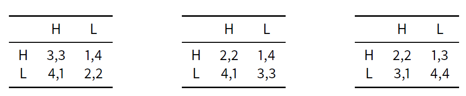
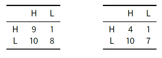
According to Gambetta and Origgi (2013), there are three possible ways to explain why, in a context such as that of Italian Academia, LL should be the expected outcome and therefore high-doers, i.e. agents who deliver H, end up being at odds. The first option is to postulate that the preferential order for most of the players is HL < LL < HH < LH (leftmost table in Table 1). This option provides an instance of the famous prisoner’s dilemma where LL is the only Nash equilibrium[10]. In this case rational agents, while preferring HH exchanges, will end up exchanging LL as a solution of this strategic game. The second possible explanation is that agents may instead have the preference ranking HL < HH < LL < LH, i.e. they eventually prefer sloppiness (LL) to perfectionism (HH). This option is instantiated by the payoffs in the central table of Table 1 (again with equal payoffs for both players). Here again LL is the only Nash equilibrium and the preference for LL is even stronger. A third possible explanation is depicted in the rightmost table and consists in players having the following preferential ranking: HL < HH < LL < LH, i.e. they prefer to be involved in an LL exchange rather than in an LH one. Using Gambetta and Origgi’s words, they are “pro-social” L-doers, as they prefer receiving L over the embarrassment of receiving H and providing L. Here too LL is a Nash equilibrium that makes players better off.
All options can explain why individuals end up delivering L. However, only the third and possibly the second option can motivate why someone who delivers L and receives H could complain. These are indeed the only cases where the LL action profile is Pareto optimal, i.e. any deviation from it would make some of the players worse off. LL is the action profile in both the center and rightmost options of Table 1 which maximizes the total utility, and this explains why it is an expected collaborative outcome.
 |
The HL framework
From our perspective, these three explanations are part of a more general scenario. Indeed, Table 1 displays only three of many games in the HL framework, i.e. the class of all the two-player games that can be defined over the actions H and L. It is important to consider this larger class because exchanges need not happen solely between players with the same payoffs, nor even with the same preferential order over action profiles. In principle, a society may be populated by individuals with quite different individual tastes. To capture such aspect, we define the type of an agent as her preferential order over action profiles (when she is player 1). We restrict ourselves to strict preferential orders, where we have 4! = 24 different types which are listed in Table 2[11].
| Type | Preferential order as player 1 | Selfishness | Mindedness | Name |
| 1 | HL<LL<HH<LH | Selfish | high | hs1 |
| 2 | LL<HL<HH<LH | Selfish | high | hs2 |
| 3 | HL<HH<LL<LH | Selfish | low | ls1 |
| 4 | HH<HL<LL<LH | Selfish | low | ls2 |
| 5 | LL<HH<HL<LH | Selfish | high | hs3 |
| 6 | HH<LL<HL<LH | Selfish | low | ls3 |
| 7 | LL<LH<HL<HH | non-selfish | high | hn1 |
| 8 | LH<LL<HL<HH | non-selfish | high | hn2 |
| 9 | LL<HL<LH<HH | non-selfish | high | hn3 |
| 10 | HL<LL<LH<HH | non-selfish | high | hn4 |
| 11 | LH<HL<LL<HH | non-selfish | high | hn5 |
| 12 | HL<LH<LL<HH | non-selfish | high | hn6 |
| 13 | LH<HL<HH<LL | non-selfish | low | ln1 |
| 14 | HL<LH<HH<LL | non-selfish | low | ln2 |
| 15 | LH<HH<HL<LL | non-selfish | low | ln3 |
| 16 | HH<LH<HL<LL | non-selfish | low | ln4 |
| 17 | HL<HH<LH<LL | non-selfish | low | ln5 |
| 18 | HH<HL<LH<LL | non-selfish | low | ln6 |
| 19 | LH<HH<LL<HL | non-selfish | low | ln7 |
| 20 | HH<LH<LL<HL | non-selfish | low | ln8 |
| 21 | LH<LL<HH<HL | non-selfish | high | hn7 |
| 22 | LL<LH<HH<HL | non-selfish | high | hn8 |
| 23 | HH<LL<LH<HL | non-selfish | low | ln9 |
| 24 | LL<HH<LH<HL | non-selfish | high | hn9 |
We adopt the following conventions (see Table 2). We call a player high-minded when its payoff for HH is greater than that for LL, and call it low-minded when HH < LL. A player is classified as selfish when the profile LH is on top of her preferences.
The full list of possible interactions among different types of players is 242=576. Gambetta and Origgi’s first explanation describes a specific game played by two hs1 players, that are both high-minded and selfish: they prefer to exchange HH over LL (high-mindedness) but nevertheless don’t mind (and indeed prefer) trading L in exchange for H (selfishness). Analogously, the second explanation describes a game played by two selfish and low-minded players of the ls1 type, while the third one describes a game among two ln5.
Having defined all types, we have not yet set the following fundamental question. What kind of strategy are two players, of any type whatsoever, going to play against each other? According to Gambetta and Origgi, both ls1 and hs1 seem conjured to play L if they are rational in the game-theoretic sense, i.e. utility-maximizers. They are indeed bound to produce the socially detrimental outcome LL, since the latter is the only Nash equilibrium of the game. Game-theoretic wisdom is arguably not the only thing that dictates peoples’ strategies [12]. However, it is fair to claim that such inference is a bit too fast in this context and that fair and pro-social behavior is instead compatible with standard rationality. Indeed, the most important for our analysis is that the life of an institution is a repeated game: co-authoring, teaching and other exchanges of this kind are very likely (or even bound) to be repeated over time. Nash equilibria and rational strategies in such repeated games are usually different from those in the one-shot case. As we show in the next section, it is not incompatible for one player to be rational and to play according to a strategy which is dictated by a fair social norm.
Repeated games and social norms
We shall focus our analysis on two types of player, the hs1 and the ls1. This allows us to analyze an interaction between high-minded and low-minded players where both types are otherwise very similar in their preferences. They are both selfish insofar as they mostly prefer delivering L and receiving H. Both also mostly dislike delivering H and receiving L. Such agents are arguably likely to be found in a competitive society where individuals are incentivized to participate in many activities (for example improving their CV by publishing, teaching, participating to conferences and research projects) while at the same time economizing their efforts and getting the most out of them.
For simplicity, we assume that their individual payoffs are on the same scale, with numerical values from 1 to 4, as described in Table 2 (where the numbers represent the payoff of player 1, i.e. the row-player).
 |
Let us look closer to the game played among two hs1. As mentioned, in an indefinitely (or infinitely) repeated game many equilibria are possible, in contrast with the one-shot case where the Nash equilibrium is LL. As a straightforward consequence of the Folk Theorem, any combination of strategies leading both hs1 to play H together most of the times leads to a Nash equilibrium for this game[13]. Therefore playing H repeatedly is reasonable in the hs1 vs hs1 repeated game. For similar reasons, playing L leads to an equilibrium in the ls1 vs ls1 game.
According to Binmore (2005, 2010), social norms are best seen as a device of equilibrium selection in a society. A social norm somehow dictates an individual strategy s for the players to follow. The combination of such individual strategies should generate an outcome which fulfills three important properties: stability, efficiency and fairness. Of course, in a context with many games and different types of players, as the HL framework, it is likely that no strategy s satisfies these properties for all possible interactions among types, and therefore there is no universal social norm. Nonetheless, some strategy can still satisfy the required properties relative to some specific game among players of the same type t, which is the case in our context. This allows us to endow different types with different norms and to work on the assumption that agents play fair, at least according to their type-specific norm.
We define a “t-norm follower” as someone who plays according to a strategy s which, if played by both players in a t vs t game, leads to
- a Nash equilibrium (stability)
- which is Pareto optimal (efficiency)
- provides player with the same payoff (fairness)
In a Nash equilibrium no player has an incentive to deviate and this is an essential prerequisite for a norm to be stable. Pareto optimality means that any deviation from s would make some of the players worse off. Thus, the condition of Pareto optimality encodes efficiency and restricts the set of Nash equilibria a society converges upon. Providing both players with the same payoff is a way of encoding fairness in an egalitarian sense, which explains why a norm becomes shared with mutual benefit[14]. We add a fourth condition on the strategy s, namely
- The strategy s allows players to minimize their loss and to possibly sanction harmful deviations. (enforcement)
The latter is a fundamental prerequisite for a norm to be enforced: deviations cause damage to someone else and should therefore be resisted. Enforcement can last only when players can endure deviations and are proactive in sanctioning them. Conditions 1-4 are altogether largely endorsed minimal criteria for a player to be a fair norm follower[15].
Back to our case, it is not difficult to see that any strategy s that dictates to play H by default and switch to L if deceived a certain number of times (i.e. if the opponent plays L and thereby diminishes my payoff) fulfills the conditions 1-4 of a fair norm among hs1 players[16]. Players sticking to a strategy of this type will be categorized as followers of an hs1-norm. The hs1-type behavior is very welcome from a societal point of view because it leads to HH exchanges, i.e. to social efficiency. Symmetrically, it is important to remark that a strategy dictating L most of the time and deviating if deceived also enforces a fair norm among ls1 (we shall call it an ls1-norm). The latter clearly does not promote social efficiency, for it induces LL exchanges.
Since we are interested in studying the impact of social norms, in what follows we assume that hs1 players follow an hs1-norm and ls1 players follow an ls1-norm, i.e. that all types are playing fair (at least according to their type). It is then interesting to see what happens when we face a clash of norms, for example when an hs1 plays against some ls1. It is not difficult to see that the initial outcome of such an exchange will be HL, i.e. very favorable to the ls1 (ls1 gets 4 while hs1 gets 1). Repeating the interaction leads the hs1 to possibly change her strategy and switch to L. The ls1 has however nothing to sanction: H is not unwelcome to her, since it generates a high payoff. Readjustment will therefore lead to LL, which is still more favorable to the ls1 than to the hs1. As a consequence, we can draw the conclusion that a ls1 who plays fair will end up being better off, in terms of interpersonal welfare comparison than an hs1 who does the same. This becomes particularly relevant if we assume, as natural, that personal welfare is an indicator of “fitness” and that more wealthy agents endure major chances of staying longer in the system. This assumption will indeed be implemented in our simulation model and will therefore provide an explanation for the dominance of the ls1 type in a society. The following more general result provides a series of sufficient conditions ensuring that a player of a given type is more fit than a player of another type. Such conditions will serve as a useful thread for our simulations.
Proposition 1. Let Player 1 follow an hs1-norm and Player 2 follow an ls1-norm. If the following conditions hold
- p2 (HL)> p1(HL),
- p2 (HL)> p2(LH),
- p2 (HL)> p2(HH) and
- p2 (LL)> p1(LL)
Proof. Since both players follow their norm, the first exchange will be HL and p2(HL) > p1(HL) by condition (a). Following her strategy, Player 2 will not switch to H since, according to conditions (b) and (c) HL is a better outcome for her than HH or LH. Player 1 may either continue playing H or switch to playing L. In the first case Player 2 gets a higher payoff, again because of condition (a). Otherwise the outcome will be LL and Player 2 is again better off than the Player 1 because of condition (d).
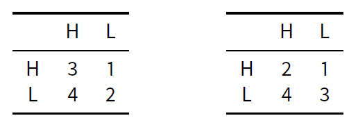
Assuming that the payoffs of both player are on the same scale, as in Table 3, the hs1 vs ls1 game is a case in point, for it satisfies the conditions (a)-(d) of Proposition 1.
We can make a similar case by framing the situation in terms of an evolutionary game. In Appendix A we show that hs1 is not an evolutionarily stable strategy against ls1. It is also interesting to analyze the replicator dynamics of a game where more than two types are involved. However, the real-life situations we would like to model are difficult to capture by purely analytic means[17]. Given the advantage of playing L and the consequent dominance of LL exchanges, we indeed want to study its consequences in more complex scenarios. Our main concern is the following: how can be an hs1-norm enforced externally, e.g. by a policy maker? This is where we need a computer model to run artificial societies. The next Section will introduce to its architecture and its main features.
Building Up an Artificial Society
Assumptions of the model
Briefly described, our model reproduces and runs an artificial society of agents of two different types[18]. Our society is intended to reproduce, at a very abstract level, the structure of a private or public organization such as a university, as in the original case study of Gambetta and Origgi (2013). The agents in the artificial society are seen as member of the organization, e.g. academic and non-academic staff in the case of Academia, who are bound to collaborate over time. Collaborations are encoded by interactions among agents. Each interaction among agents generate an individual payoff for both of them. The payoff is determined by the action profile of the interaction and the type of the agent (as specified by Table 2).
We investigate how social norms impact social efficiency when the society is populated by selfish low-doers (ls1 type following an ls1-norm) and selfish high-doers (hs1 type following and hs1-norm). Proposition 1 shows that the first type of agent has an advantage, in terms of interpersonal welfare comparison, over the second. In our model, this translates into a dominance of the first type in the long run. The model runs on the following main assumptions.
- The agents welfare is determined by their cumulative payoff, i.e. the sum of the payoffs produced by all the interactions with other agents over time
- Agents stay in the society for a limited amount of time (their working life). When they exit the society (retire), they are replaced by another agent whose type is randomly determined. The latter can be interpreted as a hiring procedure.
- Agents can retire earlier when their payoff falls under a certain threshold.
- The society has a fixed structure. The structure is determined by links between agents. Interactions among agents can only happen through the links.
- The agents play fair. Each agent follows a strategy fulfilling the conditions 1-4 of their type-specific social norm (see Sections 2.8-2.19) and never deviates from it.
- Strategies are adaptive. The choice of action takes in consideration previous interactions and is calibrated to minimize loss. Memory and calibration are determined pairwise, i.e. relative to each specific partner the agent is interacting with.
- Agents don’t know the type of the agent they are interacting with. This also means that they will not form a theory, on the basis of previous exchanges, about the strategy of the agent they are interacting with.
Description of the model
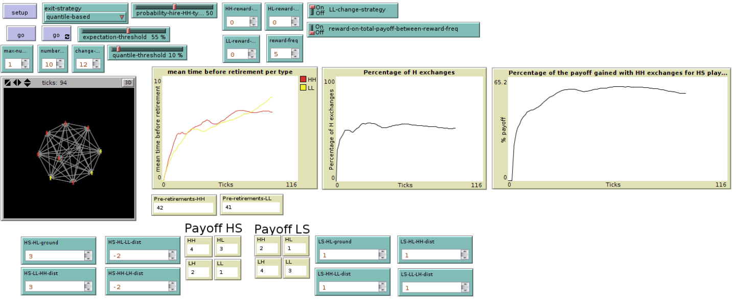
In Figure 1 the main interface of the simulation program is presented. Agents are connected by social links which enable mutual exchanges. As time passes the agents get older and, when they reach a given age, retire and are replaced by a new agent. By means of mutual exchanges the agents cumulate an individual payoff - determined by their type and the outcome of the interaction – which is meant to represent how satisfied they are in their position. When their satisfaction falls under a certain threshold they decide to pre-retire. Therefore, computing the average time before retirement for a type of agent will give us an insightful measure of how well such a type of agent fares in the society. Importantly, our model also provides the percentage of H-actions as an indicator of social efficiency. In the next paragraphs we present all these features in more detail. In Appendix B we provide the full ODD description of our model (Grimm et al. 2006) which includes the precise formulations for its most relevant operations.
Setup. The setup procedure builds a society of n agents, with n being a parameter specified by the user. In this setup agents are of two types. Types are determined by two different payoff tables that can be reset by the experimenter. The default types for most (but not all!)[19] the experiments are hs1 and ls1. Agents are connected by directed links which enable exchanges among them. The experimenter may choose to arrange links either in a totally connected or a scale-free network[20]. Exchanges happen with a certain probability determined by both the probability of one player to propose an interaction and the probability of the other player to accept it. The maximum number of interactions per agent is also determined by a parameter. The number of exchanges proposed in each round is drawn from a uniform distribution between 0 and the maximum number of interactions. In our first batch of simulations we fixed the probability of accepting an interaction to 0.5 and the maximum number of interactions to 1, so that every agent interacts, on average, with every other agent once every two rounds.
The clock. The model simulates the evolution of a society over time. Ticks are meant to represent a unit of time (one year). During each tick agents perform exchanges with their connections as determined in the setup features. After every tick agents get one year older and the system updates. At the beginning agents are assigned a random age between 25 and 65. Agents reaching the limit age of 65 retire and are replaced with a new agent. The new agent starts her career with a random age between 25 and 40 and is either a hs1 or a ls1. The type of the new agent is determined according to a probability set by the experimenter (probability-hire- hs1-type).
Exchanges and norms. Available actions for the agents are H and L. As mentioned, agents are of two types. The first type follows a hs1-norm and the second type follows an ls1-norm (Section 2.3). In the default payoff settings hs1-norm followers are hs1 and ls1-norm followers are ls1. Each exchange determines a payoff for both agents involved. The payoff of each agent is calculated according to the given payoff table. Payoff tables are set by default to the values of Table 3. The hs1-norm dictates the following strategy. The agent starts by playing H with everyone else. She keeps track, for each one of her partners pa, of the cumulative payoff she obtains by exchanging with pa. She also keeps track of the optimal cumulative payoff she should get with pa. The optimal cumulative payoff is the payoff she would have gained with a series of fair HH exchanges with another hs1-norm follower. When her actual cumulative payoff falls by a given amount under the optimal cumulative payoff she reconsiders her future action profile towards pa. This amount is fixed by a specific parameter. The procedure of reconsidering runs as follows. First, she computes (a) the payoff cumulated from the last action switch w.r.t. pa (e.g. from H to L). Then she computes (b) the payoff she would have cumulated by playing otherwise with pa (e.g. H instead of L) in the same period. The subtraction of (b) from (a) provides her the balance against pa, let us call it BALANCE(pa). If BALANCE(pa) is positive then the player keeps playing the same action, otherwise she switches. We shall call this an hs1-strategy. An hs1-strategy fulfills the conditions provided in Section 2 for being an hs1-norm: it clearly leads to a Pareto optimal Nash equilibrium among hs1 players. It also enables sanctioning and minimizing losses thanks to the reconsidering rule. Moreover, the reconsidering procedure keeps track of several factors (see Section 4) that are not considered by standard sanctioning strategies such as TIT-FOR-TAT or GRIM[21]. Therefore, it seems more adequate to describe the behavior of a rational player in this kind of situations[22]. ls1-norm followers behave analogously. They start by playing L by default and possibly switch to H. The mechanism is the same except that, in this case, a fair exchange is considered to be an LL one (ls1-strategy). Here again the ls1-strategy enforces a fair social norm among ls1 agents.
Pre-retirement rules. Two different exit strategies are available for the experimenter before setting up the simulation. The first option is a quantile-based strategy. In this mode the agent calculates her payoff at each tick and compares it with that of other agents. If her acquired payoff falls within a given percentage (selected as a parameter) of people with the lowest payoff, then she decides to pre-retire. The second option is an expectation-based strategy. The latter simply compares the agent’s actual cumulative payoff with the maximum possible cumulative payoff that she could have got from fair past exchanges (i.e. the payoff of an HH exchange for an hs1, and LL for an ls1 one). If the actual payoff falls below a given ratio of the best possible payoff then the agent decides to leave. As an additional parameter the experimenter can make the agents postpone their decision about preretirement by a given number of years[23].
Running the model. At each tick the system implements the following procedure:
- Every agent proposes a number k of exchanges to each one of its links
- accepts proposals with a given probability
- calculates her payoff
- computes her next moves according to her strategy
- decides whether to stay or to leave.
At every tick the system calculates the following:
- The mean time before retirement per type of agent.
- The percentage of H actions over time.
- The percentage of payoff gained by hs1-norm followers via HH-exchanges.
Simulation Results
First we test our analytic result of Section 2 and check whether the model confirms the analytic result of Proposition 1, i.e. that selfish low-minded agents (ls1) have an advantage over selfish high-minded ones (hs1). We test this hypothesis both on the totally connected and the scale-free network and the outcomes are quite different. The totally connected configuration confirms our analytic result. Furthermore, this advantage is quite robust and holds even by rescaling the payoff tables. Indeed, the only way to obtain an equilibrium between types is by transforming the hs1s into non-selfish agents of the types hn1 or hn2 (see Table 2). On the other hand, in the scale-free network the hs1s fare as well as the ls1s. We conjecture that this result is highly dependent on the low connectivity of the scale-free network (an average of 1.6 links per node)[24], but this should be tested further. The totally connected and the scale free network with low connectivity are two extreme cases. For most real-life social networks connectivity falls inbetween and, by consequence, in most cases ls1s keep an advantage. External policies are therefore needed to improve the situation. Hiring more hs1 agents (Section 4.2) and implementing a system of rewards and sanctions (Section 4.3) are the most intuitive options.
Basic setup
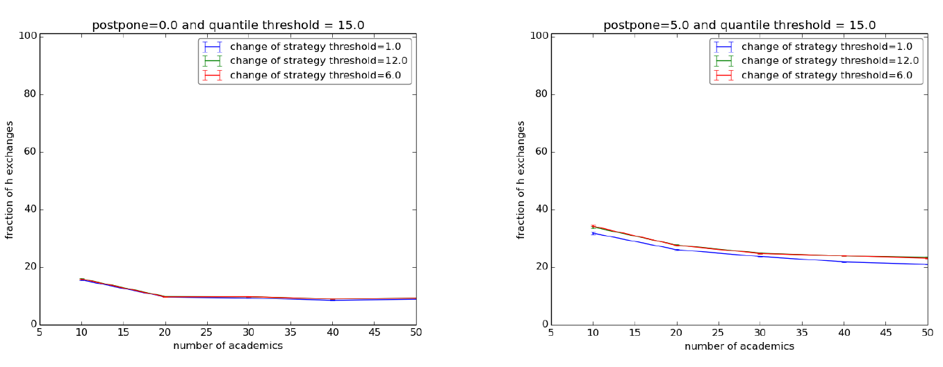
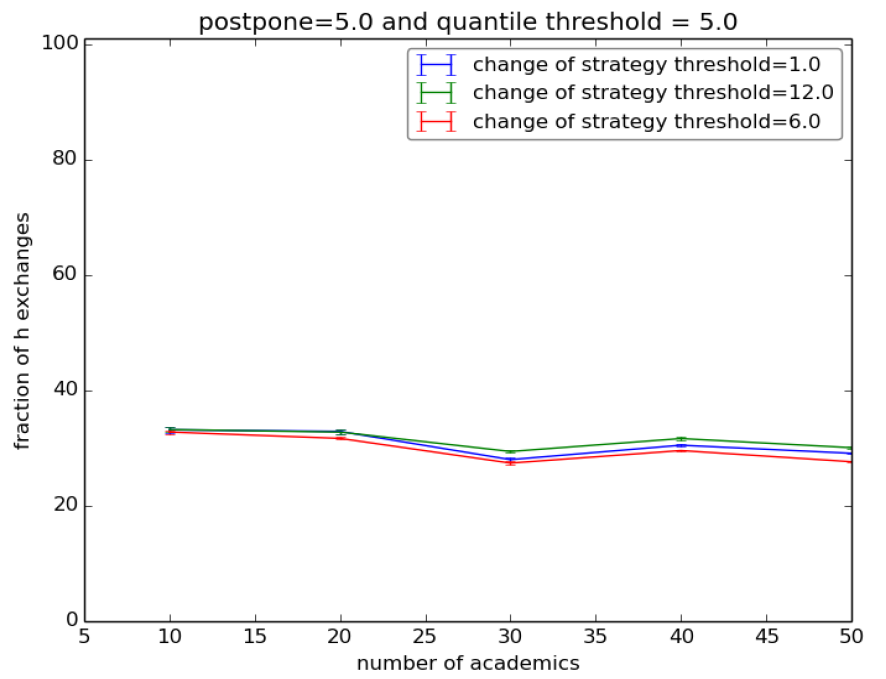
Our first setup is meant to test the fitness of the hs1 and ls1 in a totally connected network under normal conditions, i.e. where there is a fifty-fifty probability that a new agent entering in the society is hs1 or ls1, with the payoff tables set as in Table 2, under a quantile-based preretirement strategy and no additional features specified. With the help of Netlogo’s Behavior space we ran a society with 10, 20, 30, 40 and 50 individuals for 1500 ticks (a good approximation of the asymptotical behavior of the system) with 10 repetitions, which are sufficient to reach a 95% confidence interval. The change-of-strategy-threshold ranges between 1, 6 and 12[25]. The quantile ranges over 10%, 15% and 20%. We therefore get a total of 5x3x3x10 = 450 runs of the simulation. Each run tests the final value of
- the mean time before retirement for both types of agents
- the percentage of H actions
Results are quite unambiguous. When “postpone” is set to 0 the final values of the H actions fall steadily below 20% for all configurations and decrease w.r.t. the size of the society (Figure 2, left). The situation improves slightly when we set postpone to 5 (Figure 2, right) for the simple fact that hs1s endure longer. Furthermore, no matter what, the ls1 agents fare always much better in terms of mean time before retirement than the hs1s[26].
We repeated the same experiment on the scale-free configuration and the situation changes significantly. We indeed get an equilibrium between types: the rate of H actions is constantly at 50% and the mean time before retirement is the same.
These experiments indicate that, as far as selfish low-minded and selfish high-minded agents are concerned, the former have a big advantage when the connectivity is sufficiently high. Of course, this happens when the probability of both types being hired is equal and there is no external pressure or incentive by the system to modify their behavior. A provisional conclusion is therefore that, insofar as these conditions can be deemed realistic, the prevalence of low-doing is a natural outcome and low-minded people are in a better position overall.
To test the robustness of this result in the totally connected network we varied the distances among the payoff values for the agents. We tried several combinations and the outcomes confirmed the robustness of the advantage for the ls1s. Indeed, one may suspect that insofar as we validate the conditions (a)-(d) of Proposition 1 the outcome will not change much. However, quite surprisingly, the advantage was confirmed even by allowing the hs1s to get a higher payoff for LL than that of the ls1s. The latter corresponds to undermining the condition d) of Proposition 1. To do so we repeated the first experiment twice – this time with quantiles 5% and 10%[27] – by setting the payoff tables as in Table 4.
 |
In other words, we augmented the distance between the payoff of HL and LL for the hs1s while keeping the same distances for the ls1s. Distances are adjusted so that the minima and the maxima of utility are the same for both types. The results are plotted in Figure 3, and they essentially confirm the outcomes of our basic setup: with postpone 5, H actions fall steadily between 30% and 35%. Things are much worse with postpone 0.
Another way to change the situation consists of changing the type of the high-minded agents, by transforming them into non-selfish agents. To do so we transformed them into hn1 and hn2 by readjusting their payoff tables. Agents of type hn1 prefer to provide H no matter what the other provides. Agents of type hn2 do the same and even favor a fair LL exchange over the possibility of deceiving their opponent. We modified accordingly our basic experiment by setting the table for the hn1 with values LL=1, LH=2, HL=3 and HH=4 and for the hn2 with values LH=1, LL=2, HL=3 and HH=4, while leaving the ls1 table unaltered. The outcome is now of a perfect equilibrium among types (50% of H actions under all configurations) and the average time before retirement is also almost the same[28].
Under such conditions, the efficiency of an institution can be sustained if high-minded people are not selfish, we may call them “heroes” or “saints”. However, this is not end of the story. Hopefully in actual societies many different measures are taken by policy makers, research councils, employers, etc. to improve the efficiency of an institution. Any kind of evaluation, project funding, career incentive and selection process is meant to work in this direction. Such measures are often combined. The fundamental question to ask is then: what is the most effective incentive strategy? Answering this question with precision requires much more data and lies far beyond the advancement and the goals of the present work. However, we shall investigate the effects of two distinct ideal policies to see whether and to what extent they can improve the dramatic situation thus far depicted.
Possible Improvements. Introducing More hs1s.
The most natural policy for keeping up the efficiency of an institution is to try to raise the quality at the outset by a careful selection process of new employees. In our setup this corresponds to increasing the probability of introducing (hiring) an hs1 as a new agent in the society. The plots in Figure 4 show the result of varying the probability of hiring an hs1 respectively to 70% and 90% under the same setup of the first experiment with “postpone” set to 5.
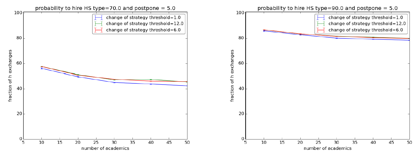
These simulations show that, in order to achieve a sensible improvement, one has to ensure a very high precision in selecting hs1 agents. Indeed, with just 70% of probability of hiring an hs1 the rate of H exchanges falls under 50% as the society grows (Figure 4, left) - and things are worse with “postpone” set to 0. With a 90% probability such rate reaches 80% (Figure 4, right) but tends nonetheless to decrease as the society grows and falls to 60% with “postpone” set to 0. Moreover, even at 90%, ls1 agents keep their advantage, since their mean time before pre-retirement is still higher (between 8 and 13 years) than that of the hs1 agents (around 6 years).
We repeated these experiments on the scale-free network and the results of Section 4.1 are confirmed: with 70% of probability of hiring an ls1 the rate of H actions raises to 70%. Analogously, it raises to 90% with a 90% probability. Again, high connectivity makes the situation worse. Furthermore, it is quite challenging for a policy maker or employer to succeed in hiring such a high percentage of high-minded individuals.
Possible Improvements. Rewards and Sanctions.
Another way of promoting the efficiency of an institution is to implement a system of rewards (promotions, monetary rewards, facilities etc.) and sanctions (firing, fines or any kind of negative reward). In our setting, this amounts to modifying the payoff attributed to agents as a consequence of their behavior. The functioning of actual rewarding systems can be quite complex and its consequences on the individual satisfaction very hard to measure. For the purposes of this initial stage of our research we choose to implement an ideal mechanism. Such a mechanism keeps track of every exchange among the agents and rewards them with a probability proportional to the number of high-quality exchanges they have been involved in. Such a rewarding system is idealized insofar as it is perfect in recognizing and rewarding high quality.
Our mechanism of rewards and sanctions consists of proportional raises and decreases of the agent’s payoff. Each agent can be rewarded for the HH exchanges he has taken part in. Analogously he can be sanctioned for the LL exchanges. The frequency with which rewards and sanctions are attributed is an experimental parameter. The amount of the reward (sanction) is calculated every f years and is a percentage of the payoff cumulated by the individual during f. Such a percentage is also a parameter. Additionally, the reconsidering procedure of agents now also takes into account whether a certain agent contributed to rewards (sanctions), thus enabling a change in strategy towards this individual[29]. For a detailed description of the reconsider procedure, and the reward procedure, please refer to Appendix B.
Bringing back the probability of hiring hs1s to 50% we then tried the following experiment. We fix a society of 30 agents with a quantile pre-retirement threshold fixed at 15%. The change-of-strategy threshold is fixed at 6. The frequency of rewards and sanctions varies: it is either every tick or every 3 ticks. The reward for HH exchanges varies in the range 50% and 100%. The sanction for LL exchanges varies between 0%, -50% and -100%.
| (Frequency of the reward=3.0) | Reward for doing HH exchanges=100.0 | Reward for doing HH exchanges=50.0 |
| Punishment for doing LL exchanges | Fraction of h exchanges | Fraction of h exchanges |
| 0.0 | 10.1 (0.05) | 9.85 (0.03) |
| 50.0 | 17.96 (0.14) | 17.85 (0.19) |
| 100.0 | 19.33 (0.13) | 19.34 (0.17) |
| (Frequency of the reward=1.0) | Reward for doing HH exchanges=100.0 | Reward for doing HH exchanges=50.0 |
| Punishment for doing LL exchanges | Fraction of h exchanges | Fraction of h exchanges |
| 0.0 | 12.66 (0.45) | 10.14 (0.03) |
| 50.0 | 75.81 (0.16) | 39.73 (0.43) |
| 100.0 | 80.91(0.08) | 65.44 (0.17) |
The results of this simulation show that in order to achieve a percentage of H exchanges above 50% we should couple high rewards (above 50% for HH exchanges) with consistent sanctions (above 50% for LL exchanges) and with high frequency (Table 6). Indeed, as soon as the rewarding frequency is set to 3 ticks all benefits tend to vanish (Table 5).
Finally we also tried to change the probability of hiring hs1s to 65% to check the benefits of a combined policy. Results are presented in Table 7 and 8. As shown, the situation improves with respect to the equal probability case and seems to be less dependent on the frequency of rewards and sanctions.
| (Frequency of the reward=3.0) | Reward for doing HH exchanges=100.0 | Reward for doing HH exchanges=50.0 |
| Punishment for doing LL exchanges | Fraction of h exchanges | Fraction of h exchanges |
| 0.0 | 16.47 (0.12) | 14.96 (0.07) |
| 50.0 | 53.98 (0.29) | 53.68 (0.29) |
| 100.0 | 62.52 (0.36) | 61.31 (0.32) |
| (Frequency of the reward=1.0 ) | Reward for doing HH exchanges=100.0 | Reward for doing HH exchanges=50.0 |
| Punishment for doing LL exchanges | Fraction of h exchanges | Fraction of h exchanges |
| 0.0 | 83.01 (0.4) | 17.11 (0.11) |
| 50.0 | 87.28 (0.1) | 64.84 (0.21) |
| 100.0 | 88.81 (0.6) | 76.85 (0.1) |
Discussion and Conclusions
The initial input for our work was to analyze and test Gambetta and Origgi’s game-theoretic explanations for the odd dynamics and the inefficiency of Italian academia. The first outcome of our analysis (Proposition 1) leads to a more general insight. Insofar as the HL framework is a reliable approximation of the “game of life” in certain communities, the advantage of low-doing is an extreme one. We suspect that a similar problem undermines the efficiency and quality standards of many organized groups and institutions. Indeed, assuming that both high-minded and low-minded individuals are selfish, and nevertheless play according to social norms in their type-specific way, the low-minded ones have a consistent advantage, in terms of interpersonal welfare comparison, and social efficiency gets radically compromised.
This incentivized us to test the HL framework at work in complex artificial societies where the programmer can modularly bring in additional factors in order to represent more articulated scenarios. Our first batch of simulations - where the hs1s and ls1s are equally likely to enter the system - confirms our analytic result (Proposition 1), but only in cases of high connectivity. Furthermore, it shows that, as the society develops, the hs1s are even worse off. Therefore, the larger the collectivity the milder the advantage of hiring more high-minded individuals. The only way, under these conditions, to reach an equilibrium between types is to modify the payoff settings for the high-minded agents and transform them into “heroes” and “saints” (hn1 and hn2) which, the reader may agree, is unrealistic for a society to have.
For a second and third batch of simulations we modified our settings and allowed for external interventions – meant to model the action of a policy-maker – such as raising the probability of hiring hs1 agents and introducing a system of rewards and sanctions. Under external influence the system can improve its efficiency to higher standards. There is, however, an argument for claiming that both strategies are quite expensive for a policy-maker. The best combination of strategies is still unknown and further policies are to be tested. Another problematic point is that both kinds of external influence are implemented by an ideal policy-maker, i.e. someone that has full knowledge of the state of the system and can distinguish perfectly high quality from low quality. Both features are quite unrealistic. Intuition tells instead that evaluations and decisions are often made under partial ignorance and are also biased by the evaluator’s preference: only in ideal cases one may hope to have an expert evaluation committee composed only by high-minded and totally knowledgeable members. This problem is a version of the dilemma quis custodies ipsos custodies. In future research we aim to study, within our model, the effects of more realistic and fallible systems of rewards. Other interesting venues consist of studying more specific instances of our game and of using our model to test the effect of different social norms in action.
We conclude with some considerations on the case of Italian academia which inspired our work. Structural problems of the Italian research system are one major cause of its “brain drain”. The latter is a constant object of debate in media, newspaper articles and books (Di Giorgio 2003) as well as articles in scientific journals (Abbott 2001; Battiston 2002; Burr 2004; Morano-Foadi 2006). Individual reports of Italian researchers working abroad stress, as the major “push” factors to leave Italian academia, the absence of meritocracy, nepotism, the baron system and, last but not least, the scarcity of funding (Morano-Foadi 2006)[30]. In one sense nepotism and the baron system are based on a strong link of loyalty between parties: the professor promotes the careers and secures the position of those who collaborated with him (or her) over several years and adapted to their standards. Arguably, the scarcity of investments and resources is likely to emphasize the dominance of a group when this is already in place: the few positions and allocated funds are to be secured to the members of the group who abide by the law (Morano-Foadi 2006). By consequence, different cultures or clusters are unlikely to emerge in the system. To this we must add a long-term resilience to external evaluation in many sectors (Boffo and Moscati 1998). All these causes are complex to disentangle and some of them seem to be correlated. Our analysis provides a general clue to understand how they come together. Academia, as well as other institutions, is made of different “cultures”, i.e. groups holding to different standards of efficiency and cooperation. Each of these cultures is likely to promote a different ingroup social norm. Deviations from the ingroup norm tend to be resisted and outsiders are often sanctioned by other ingroup members, e.g. in the ways documented by Gambetta and Origgi. Sanctioning becomes marginalization when the ingroup culture is largely dominant in the society. However such dominance need not be the outcome of an evil global plan, for it may only reflect a natural tendency of the system[31].
Acknowledgments
The authors thank Prof. Erik J. Olsson and Dr. Jeroen Smid for many inputs and improvements of this paper. Work by Carlo Proietti was supported by the Riksbankens Jubileumsfond (P16-0596:1).Notes
- The tragedy of commons is a social dilemma introduced and explored by the economist G. Hardin (1968). Hardin’s analysis originates from the insight of W.F. Lloyd (1833). Lloyd analyses the possible effects of unregulated grazing over common fields. He remarks that, when the individual advantage of a certain extent of free-riding, e.g. grazing some sheep in a common parcel for cows, overrides the loss induced by spoiling the common good then individuals may easily destroy the shared resource.
- The term "amoral familism" was coined by E. Banfield in his book The moral basis of a backward society (1958). Amoral familism amounts to the maxim "Maximize the material, short-run advantage of the nuclear family; assume that all others will do likewise". Banfield employs it to explain the backwardness of certain rural societies in southern Italy. Backwardness would have been very difficult to understand otherwise, especially in the light of the welfare of other rural communities with similar initial conditions.
- As witnessed by many reports of Italian researchers in Italy and abroad, misbehavior is not only deeply rooted but also largely justified in Italian Academia. For example, the authors illustrate several cases of public debate over complaints of plagiarism where most of the arguments go in defense of plagiarists and against whistle-blowers or victims. "We investigate a phenomenon which we have experienced as common when dealing with an assortment of Italian public and private institutions: people promise to exchange high quality goods and services (H), but then something goes wrong and the quality delivered is lower than promised (L). While this is perceived as ‘cheating’ by outsiders, insiders seem not only to adapt but to rely on this outcome. They do not resent low quality exchanges, in fact they seem to resent high quality ones, and are inclined to put pressure on or avoid dealing with agents who deliver high quality". (Gambetta and Origgi, 2013, p. 3).
- Three such conditions encode stability, efficiency and fairness, as specified by Binmore (2005, 2006, 2010). Alternative game-theoretic accounts of normativity have been recently formulated – e.g. Bicchieri (2006, 2010) and Gintis (2009, 2010) – which may not fully agree with one another, as shown by Paternotte and Grose (2013). It is not among our present purposes to give a fully developed definition of the notion of social norm nor to discuss the pros and cons of the competing approaches. However, the minimal conditions we set for agents to be norm-followers are agreed upon by all mainstream accounts of normativity.
- Our model is available at https://www.openabm.org/model/5120/version/1/view.
- As explained by Gambetta and Origgi (2013), this is a strong simplification (maybe too strong in those contexts where the quantities of deliverable goods are finely scalable) but good enough for the points we want to make. Alternatively one might read H as “work in accordance with the best of the agent’s abilities” and L as the negation of H.
- This is, again, a simplification leaving out some specific types of exchanges such as coauthoring among more than two individuals.
- We remark however that our model of Section 3 is not bound to such restriction.
- Here player 1 is the row player and player 2 is the column player and the payoffs of both are associated to each of the four possible outcomes (the ones on the left for player 1 and the ones on the right for player 2).
- A Nash equilibrium is an action profile for which no player has an incentive to be the only one who deviates. We can easily check that this is the case for LL in the leftmost table. Indeed, both players get 2 and would get less (namely 1) by playing H instead. On the contrary, HH is not a Nash equilibrium, although providing a better payoff for both players, because anyone would be better off by being the one to play L, i.e. she would get 4 instead of 3.
- The full HL framework has a larger cardinality. This restriction excludes for example the well-known Hi-Lo game where the preferences for both players are HL = LH < LL < HH.
- Among other things, experimental evidence on actual social groups shows that agents most often avoid "rational moves" that are perceived as unfair, e.g. when they are put in strategic settings like the Ultimatum game (see Sanfey et. al. 2003). Such results are usually interpreted as demonstrating a deeply rooted sense of normativity or sociality in human agents, which should partly compromise with their game-theoretic wisdom.
- The payoff of both players in this case dominates the minmax profile (LL) and this is a sufficient condition for it to be a Nash equilibrium in the repeated game. Moreover, if the player gives a sufficiently high value to the payoff earned in future exchanges with respect to the payoff of his next move, then the former condition becomes also a necessary one. See Fudenberg and Tirole (1991).
- There are many alternative ways of encoding fairness in philosophical literature. J. Rawls (1971) is probably the most prominent contemporary defender of an egalitarian conception of fairness. On the contrary, Harsanyi (1976) defends a utilitarian reading of it, i.e. fairness as maximization of total utility. We don’t take a stand in this discussion here. We only point out that, in our specific case, where both players have the same scaling of individual payoffs, the t-norms we will introduce turn out to be fair both in an egalitarian and utilitarian sense.
- They surely are in the game-theoretic framework of Binmore (2005). Prima facie it seems that this is not the case for other accounts of social norms such as for Gintis (2009, 2010, 2011) and Bicchieri (2006, 2010), as stressed by Paternotte and Grose (2013). For example, Gintis sees social norms as “choreographers”, inducing a correlated equilibrium on a game G. The latter becomes the central notion instead of that of Nash equilibrium. However, a correlated equilibrium on a game G is still described as a Nash equilibrium of a larger game G+. To some extent, this is analogous to what happens when one transforms a one-shot game into a repeated one. In general, most of the examples provided by both Bicchieri and Gintis 2-4 are also satisfied.
- We shall expand more on this point in Section 3.
- The study of replicator dynamics for the HL framework is a very interesting subject in itself but it would carry us too far away from our present concern. We therefore leave it for future work.
- Readers have access to the simulation file through https://www.openabm.org/model/5120/version/1/view.
- In Sections 4.2-4.9 we perform experiments with other type of players, namely, hn1 and hn2.
- The nature of an exchange is left unspecified at this stage. While totally connected networks approximate situations of full collaboration within a group, scale-free networks are best suited to capture, e.g., social dynamics as co-authoring, where some agents are more connected than others and a power-law structure applies. Modelling more specific dynamics may require a more sophisticated structure for the social network.
- Both the hs1-strategy and the ls1-strategy allow agents to change their action after some point to minimize their loss. However, in Section 4 we shall introduce some modifications (sanctions and rewards) that push agents to further considerations and allow them to possibly flip their action back in order to improve their payoff.
- The kind of strategy described is indeed very close to the no-regret-learning method (see Hannan 1957 and Hart 2000).
- Making the agents postpone their decision about pre-retirement by a sufficient number of years immunizes them (and the outcome of an experiment) from some unwanted initial side effects, i.e. it helps the steady state not to be dependent on the transient states (see Section 4).
- To generate a scale-free network here, we used the Barabási & Albert (2002) algorithm. It generates a scale-free network with an exponent of 3. If N is the number of nodes, the average connections a node has is \(\sum_{k=1}^N k^{-\alpha +1}\). It quickly converges to about 1.6 as N increases.
- Different thresholds stand for different levels of adherence to a norm. If the threshold is set to 1 then the agent will revise her future action profile immediately after the first loss. On the other hand, when the threshold is set to 6, the agent will revise only after losing 6 units w.r.t. the maximum payoff given by fair exchanges. In our setup agents exchange in average once every two ticks. This means that hs1 agents, by losing 2 units each time, will wait in average 6 ticks before reconsidering their action.
- The average time before retirement for the hs1s ranges between 2 and 1 with postpone 0 and between 4 and 5 with postpone 5. Instead, ls1s retire after around 8-10 ticks with postpone 0 and 10-14 with postpone 5.
- We tried a lower quantile threshold to make exit conditions quite relaxed for the agents. Indeed, repeated trials showed that after some point the ls1s start to take over numerically. We therefore wanted to allow the hs1s more chances to survive longer in the game.
- Anecdotal evidence may give a hint for this result. The authors have experienced various examples of zealous functionaries who, working alone and following the call of duty, contribute to keep up dysfunctional institutions to an acceptable level of efficiency.
- The agent spreads the value of her reward or sanctions for exchanges of type XX (i.e. HH or LL) over all the agents active in exchanges of type XX. This action counteracts the change of strategy triggered in order to contain the losses. We have seen that an hs1 agent will play L against an ls1 agent when the loss due to playing H falls beyond the change of strategy threshold. However, if the sanction due to playing L imbalances the loss, the hs1 agent will go back playing H even with ls1 agents.
- The scarce allocation of funds to research and development is most likely to be a major cause of inefficiency. According to most recent data provided by the Italian agency for the evaluation of the university and research system (ANVUR), the percentage of GDP allocated by the Italian government to research and development is 1.27% over the years 2011-2014, where the average of the OECD countries is 2.23%.
- The so-called Baroni in Italian Academia are representatives of a system of specific hierarchical relationships between professors and assistants, which was dominant and is still present in certain areas of Academia in many countries.
- If we have a discrete probability distribution \(Pr\{x=i\}\) in support of a domain \(D\), then the expected value will be \(E[x]=\sum_{i\in D}i*Pr\{x=i\}\).
Appendix
A - Why hs1 is an evolutionarily unstable strategy
In an evolutionary setting we can divide the population into two main strategies, hs1 and ls1. We can represent their fitness as the minimal payoff they get after a sufficiently long series of exchanges based on the social norms described in Section 2. This gives the following payoff table.
| hs1 | ls1 | |
| hs1 | 3,3 | 2,3 |
| ls1 | 3,2 | 3,3 |
According to evolutionary game theory (Weibull 1997) HS is an evolutionarily stable strategy if and only if either
- (\(p_{1}(hs1, hs1)\) > \(p\_{1}(ls1, hs1)\)
- \(p_{1}(hs1, hs1)\) = \(p_{1}(ls1, hs1)\) or
- \(p_{1}(hs1, ls1)\) > \(p_{1}(ls1, ls1)\)
B - ODD protocol
Overview
Purpose
The purpose of the model is to understand how the social norms followed by two different types of individuals affect the efficiency of an institution and determine the dominance of one type over the other. Individuals are either low-minded or high-minded. Low-minded individuals prefer collaborating with others providing low quality of a given good and receiving low quality over providing high quality and receiving high quality. The contrary holds for high-minded individuals. Both types of individuals are pro-social in the sense that their attitude is fair, stable and efficient when they collaborate with individuals of the same type.
State variables and scales
The model comprises a single level of entities, individuals and links among them. Individuals are characterized by state variables that determine their identity (one of two types), age and payoff (per single time unit and cumulative) and a number of variables used to store information about agents they are linked to. Links enable collaborations among two individuals and are characterized by state variables that determine the number of collaborations to propose (from one individual to the other), the probability of accepting a collaboration and the number of collaborations in common. Global variables are used to account for the payoff tables of the individuals as well as a number of statistics. A complete list of the variables employed is reported in Table 10.
| Variable | Description |
| Agent variables | |
| type-of-academic | LL or HH etc. |
| number-of-collaborations | Number of total collaborations |
| age | Age in ticks |
| age-hired | Age at which the agent was hired |
| total-payoff | Total payoff earned so far |
| payoff-this-year | Payoff only for this year |
| payoff-between-rewards | Maps payoff between two reward times |
| difference-from-optimal-per-agent | Maps other agents to the difference from the optimal payoff cumulated so far. It Is reset each time the agent changes strategy |
| my-id | Agent ID |
| type-of-exchange-to-number-of-exchanges | Maps the type of exchanges to the number of exchanges of that type |
| type-of-exchange-to-ids | Maps the type of exchanges to ids (not necessari-ly unique) – It is reset every reward period is done. |
| payoff-per-type-of-exchange | Maps the type of exchange to the payoff gained doing that type of exchange |
| payoff-per-type-of-exchange-between-rewards | Maps the type of ex-change to the payoff gained doing that type of exchange between two reward times |
| percentage-of-payoff-per-type-of-exchange | Maps the type of exchange to the percentage of the payoff gained by doing that type of exchange |
| real-exchanges-to-id | Maps ids to the map (exchanges -> number of ex-changes of that type). It Is reset per agent when a reconsideration is done. |
| saldo-per-agent | Maps the other agents to the saldo so far |
| counterfactual-payoff-between-rewards | Accounts for the payoff the agent would have gained by exerting the counterfactual strategy between reward times. |
| counterfactual-payoff-per-type-of-exchange-between-rewards | Accounts for the payoff the agent would have gained by exerting the counterfactual strategy between reward times, subdivided by type of exchange. |
| delay-counter | Time before executing the first change |
| Link variables | |
| probability-of-acceptance | Probability of accepting a collaboration |
| collabs-to-propose | Number of collaborations to propose per link |
| collabs-in-common | Number of collaborations in common |
| Global variables | |
| types-of-academics | LL HH etc.. |
| color-of-types | Color of LL HH etc.. |
| age-of-retirement | Maximum age to exit academia |
| age-min | Minimum age to enter academia |
| payoff-tables | Maps type of academic to payoff tables |
| payoff-table-HH | Table of payoffs for HH |
| payoff-table-LL | Table of payoffs for LL |
| strategy-index | Maps strategy name to index |
| number-of-exchanges-per-type | Maps strategy used to the number of times the strategy was used |
| number-of-retirement-per-type | Maps type to the number of retire-ments |
| number-of-pre-retirement-per-type | Maps type to the number of pre re-tirements |
| mean-time-before-retirement-per-type | Maps type to the mean time be-fore retirement |
| payoffs-this-year | List of payoffs this year |
| number-of-pre-retirement-this-year-per-type | Maps type to the number of pre retirements this year |
| number-of-pre-retirement-per-year-per-type | Maps type to the number of pre retirement per year (list) |
| mean-number-of-pre-retirement-per-type | Maps type to the mean number of pre retirements per year |
| h-fraction | Fraction of h exchanges |
| average-payoff-HH-for-HH | Average payoff gathered by HH exchanges by HS players |
Process overview and scheduling
The model proceeds in annual time steps. At every time step every agent performs the following sequential actions
- Proposes/accepts exchanges from the agents it is connected to.
- Perform the exchanges according to its strategy. Possible actions for the agent are L (delivering low quality) or H (delivering high quality)
- Recalculates its own strategy for the next year.
- Ages one year.
- Updates its stats, according also to rewards/fines received.
- Considers pre-retirement, or, if it has aged to the threshold limit, retires.
Design Concepts
Emergence: Population dynamics emerge from the behavior of the individuals. An individual’s life cycle depends heavily on the other agents’ behavior, although their type, assigned at the beginning, according to a probability, dictates the individual’s behavior. Adaptation and fitness-seeking are dictated by the agent type.
Sensing: Individuals are assumed to know their own type, payoff accumulated and their age. They also keep track of the other agents’ behaviour in past interactions over a limited time span and adjust their behaviour consequently.
Prediction: Agents just react to the other agents’ past actions.
Interaction: Individuals propose, accept or deny exchanges proposed by agents linked to them.
Stochasticity: The type of a new agent in the society is determined by a probability distribution. In addition, the frequency of exchanges, the change of behavior by the agents and the allocation of rewards and sanctions are drawn from a probability distribution. This is done in order to avoid systematic deterministic results and to test the robustness of high-minded agents under many possible configurations.
Observation: Only population-level variables are recorded, i.e. mean time before retirement, and percentage of HH exchanges over the total number of exchanges.
Details
Initialization
A network of agents of the two types is laid out. The proportion of agents of the two types is the function determined by a probabilistic parameter. The agents’ initial age is randomly assigned and varies between 25 and 40. The network can be either totally connected or laid out as a power law, depending on the initial settings.
Input
Periodically, rewards and penalties are assigned to agents in the form of additions or subtractions from their cumulative payoff. The time between assignments is driven by an input parameter. The amount of the rewards/penalties is given as an input, depending on how many exchanges of type HH or LL they performed between two reward/penalty times. The amount of rewards and penalties impacts the agent’s decision of future actions by means of the Reconsider procedure (see Submodels).
Submodels
Rewards: The mechanism works as follows. We call \(\mathbf{A}\) the set of agents active between two rewarding times. For each \(p\in\mathbf{A}\), let \(N_{xx}^p\) be the number of exchanges of type XX (e.g. HH) between two rewarding times of agent p. Let \(P_{xx}^p\) the probability of getting a reward (resp. sanction) per exchange of type XX for agent a between two rewarding times. We calculate the latter as \(\frac{N_{XX}^p}{\max_{p'\in A} N_{XX}^{p'}}\), i.e. the ratio between the XX exchanges performed by the agent between two rewarding times, and the maximum of XX exchanges of all the agents active between those rewarding times. The jest behind this choice is to give a higher reward to the relatively more efficient agents as it should happen in a fair and proportional rewarding system.
Reconsider: Given the presence of rewards and sanctions, we consider it to be natural that agents should weigh them when reconsidering whether or not to change their actions towards a given opponent \(p\). When the agent reconsiders, she takes into account how much she gained by pursuing her actions from her last reconsideration and how much she would have gained, by pursuing the opposite actions. More formally, if the real actions before the last reconsideration are \(a=\{a_i,a_{i+1},\dots,a_k\}\), the opposite actions would be \(\acute{a}=\{\acute{a}_i,\acute{a}_{i+1},\dots,\acute{a}_k\}\), where the bar operator denotes the opposite of the non-barred action, e.g. \(\acute{H}=L\).
The agent computes the payoff she has gained from her last reconsideration \(u_j(a)\), and the payoff she would have gained pursuing the opposite actions \(u_j(\acute{a})\) without taking into account rewards or sanctions. Then she computes the expected reward/sanction[32]. If we have a discrete probability distribution \(Pr\{x=i\}\) in support of a domain \(D\), then the expected value will be \(E[x]=\sum_{i\in D}i*Pr\{x=i\}\).} she would gain if there would be given rewards and sanctions at this moment, due solely to her opponent, given her actions \(E[r_j(a)]\), and the expected reward/sanction she would have gained by pursuing the opposite actions, if there would be given rewards and sanctions at this moment, due solely to her opponent \(E[r_j(\acute{a})]\). She then computes \(u_j(a)+E[r_j(a)]-u_j(\acute{a})-E[r_j(\acute{a})]\) and if this sum is less than 0, she plays the opposite of the last action she played.
References
ABBOTT, A. (2001). Forza scienza!. Nature, 412(6844), 264-265. [doi:10.1038/35085639]
ALBERT, R. & Barabási, A.L. (2002). Statistical mechanics of complex networks. Reviews of Modern Physics 74(1), 47-97 .
BANFIELD, E.C. (1958). The Moral Basis of a Backward Society. Glencoe, IL: The Free Press.
BATTISTON, R. (2002). A lament for Italy’s brain drain (Book Review), Nature 415(6872), 582-83.
BICCHIERI, C. (2006). The Grammar of Society: The Nature and Dynamics of Social Norms. Cambridge, MA: Cambridge University Press.
BICCHIERI, C. (2010). Norms, preferences, and conditional behavior. Politics, Philosophy & Economics, 9(3), 297-313.
BINMORE, K. (2005). Natural Justice. Oxford: Oxford University Press. [doi:10.1093/acprof:oso/9780195178111.001.0001]
BINMORE, K. (2006). Why do people cooperate?. Politics, Philosophy and Economics, 5 (1), 81-96.
BINMORE, K. (2010). Social norms or social preferences?. Mind & Society, 9(2), 139-157. [doi:10.1007/s11299-010-0073-2]
BOFFO, S. & Moscati, R. (1998). Evaluation in the Italian Higher Education System: many tribes, many territories... many godfathers. European Journal of Education, 33(3), 349-360.
BURR, D. (2004). Injustice of draft law will speed Italy's brain drain. Nature, 428(6986), 891-891. [doi:10.1038/428891b]
DI GIORGIO C. (2003). Cervelli export: perché l'Italia regala al mondo i suoi talenti scientifici. Rome, Italy: Adnkronos libri.
ELSTER, J. (1989). The Cement of Society: A Survey of Social Order. Cambridge, MA: Cambridge University Press. [doi:10.1017/CBO9780511624995]
FUDENBERG, D. & Tirole, J. (1991). Game theory (Vol. 1). Cambridge, MA: The MIT Press.
GAMBETTA D. & Origgi G. (2013). The LL Game: the curious preference for Low quality and its norms, Politics, Philosophy & Economics 12(1), 3-23. [doi:10.1177/1470594X11433740]
GINTIS, H. (2009) The Bounds of Reason. Princeton, NJ: Princeton University Press.
GINTIS, H. (2010). Social norms as choreography. Politics, Philosophy & Economics, 9(3), 251-264. [doi:10.1177/1470594X09345474]
GINTIS, H. (2011). Reply to Binmore: Social Norms or Social Preferences?. Accessible online at: http://www.umass.edu/preferen/gintis/ReplayToBinmore.pdf.
GRIMM, V., Berger, U., Bastiansen, F., Eliassen, S., Ginot, V., Giske, J., Goss-Custard, J., Grand, T., Heinz, S. K., Huse, G., Huth, A., Jepsen, J. U., Jørgensen, C., Mooij, W. M., Müller, B., Pe’er, G., Piou, C., Railsback, S. F., Robbins, A. M., Robbins, M. M., Rossmanith, E., Rüger, N., Strand, E., Souissi, S., Stillman, R. A., Vabø, R., Visser, U. & DeAngelis, D. L. (2006). A standard protocol for describing individual-based and agent-based models. Ecological modelling, 198(1), 115-126. [doi:10.1016/j.ecolmodel.2006.04.023]
HANNAN, J. (1957). 'Approximation to Bayes risk in repeated play.' In M. Dresher, A. W. Tucker & P. Wolfe (Eds.), Contributions to the Theory of Games, Vol. III, Princeton, NJ: Princeton University Press, pp. 97-139.
HARDIN, G. (1968). The tragedy of the commons. Science, 162(3859), 1243-1248. [doi:10.1126/science.162.3859.1243]
HARSANYI, J. C. (1976). Essays on Ethics, Social Behaviour, and Scientific Explanation (Vol. 12). Dordrecht/Boston, MA: Reidel.
HART, S. & Mas-Colell, A. (2000). A simple adaptive procedure leading to correlated equilibrium. Econometrica, 68(5), 1127-1150. [doi:10.1111/1468-0262.00153]
LLOYD, W. F. (1833). Two Lectures on the Checks to Population. Oxford: Colingwood.
MORANO-FOADI, S. (2006). Key issues and causes of the Italian brain drain. Innovation, 19(2), 209-223. [doi:10.1080/13511610600804315]
PATERNOTTE, C. & Grose, J. (2012). Social Norms and Game Theory: Harmony or Discord?. The British Journal for the Philosophy of Science, 64(3), 551-587.
RAWLS, J. (1971). A Theory of Social Justice. Cambridge, MA: Belknap Press.
SANFEY, A.G., Rilling, J. K., Aronson, J. A., Nystrom, L. E., & Cohen, J. D. (2003). The neural basis of economic decision-making in the ultimatum game. Science, 300(5626), 1755-1758.
WEIBULL, J.W. (1997). Evolutionary Game ttheory. Cambridge, MA: MIT Press.