
Introduction
Spatial agent-based models (ABMs) are capable of investigating the emergence of complex phenomena, such as land-use change, that result from many distributed interactions between heterogeneous agents and their environment, which are not well represented by top-down statistical or general equilibrium modeling approaches (Irwin et al. 2009; Huang et al. 2014). Many spatial ABMs are characterized by multi-level and nonlinear interactions, emergent behavior, and path-dependent outcomes (Brown et al. 2005; ten Broeke et al. 2016). While these features are often desirable to capture salient features of real systems, model complexity makes it difficult to deconstruct sources of model output sensitivity in relation to variation in inputs. This task is particularly important when transitioning from a conceptual to empirically parameterized model. When data collection is costly, such as attaining behavioral data for ABMs from surveys, sensitivity analysis is a beneficial step to identify parameters responsible for model sensitivity and prioritize data collection efforts to constrain those variables. This paper demonstrates the synergies of integrating two different methods for sensitivity analysis to achieve a comprehensive investigation of spatial and temporal sensitivities of an established conceptual ABM for moving towards a more empirically grounded model.
Standardized methods for sensitivity analysis for ABMs are still developing (see ten Broeke et al. 2016; Thiele et al. 2014), but there is a wealth of knowledge to draw from in the broader environmental modeling field. Global sensitivity analysis (GSA) is a relatively well-developed methodological area for investigating how variation in model inputs leads to model output variation (Brugnach 2005; Cariboni et al. 2005; Marino et al. 2008; Pianosi et al. 2016; Sarrazin et al. 2016). GSAs are implemented through a set of mathematical techniques designed to quantify the relative contributions of and propagation of uncertainty from individual model parameters and their interactions with other parameters through a comprehensive sweep over the parameter space (Ligmann-Zielinska and Sun 2010; Pianosi and Wagener 2015). This is distinct from simple one-factor-at-a-time (OAT) methods, which are more suitable for exploring individual parameter effects on outcomes (e.g., scenario analysis) (ten Broeke et al. 2016). A wide array of GSA methods exist that range from simple parameter perturbation to variance decomposition, and are designed for equally diverse purposes ranging from model fitting to understanding the robustness of model outcomes across parameter values (Pianosi et al. 2016; ten Broeke et al. 2016). GSA methods have recently been reviewed in detail in by Pianosi et al. (2016). A variety of GSA techniques for specifically analyzing spatial and/or temporal model sensitivities have also been developed and reviewed elsewhere in detail (Saltelli et al. 2008, 2010; Lilburne and Tarantola 2009). However, these GSA methods may not be sufficient to address the unique challenges of ABMs (ten Broeke et al. 2016), and the few recent efforts to apply GSA methods to spatial ABMs demonstrate the inadequacy of any single existing GSA method (e.g., Lilburne and Tarantola 2009; Ligmann-Zielinska 2010, Saltelli et al. 2010; Ligmann-Zielinska 2014a; 2014b; Thiele et al. 2014). Thus, understanding of the sensitivities of many spatial ABMs in use today remains limited (Ligmann-Zielinska and Sun 2010).
Variance- and density-based GSA
Two broad approaches to GSA, variance- and density-based, have been most often applied to spatial environmental models. Variance-based GSA quantifies the sensitivity of outcome variance attributed to variability in model inputs, and has the advantage of being both model independent and relatively easy to implement through the calculation of variance sensitivity indices (Ligmann-Zielinska and Sun 2010; Saltelli et al. 2010; Pianosi and Wagener 2015). However, the generation of sufficient model output to obtain accurate sensitivity estimates with variance-based approaches can be computationally expensive, particularly for sophisticated models with high levels of parameter interactions (e.g., Baroni and Taratola 2014 required 7,168 model evaluations for 5 uncertain inputs). Additionally, variance-based analysis assumes output variance is a reliable sensitivity measure, but this may not be the case when model outcomes display skewed or multi-modal distributions (Pianosi and Wagener 2015).
Non-normal outcome distributions are commonly observed in complex systems due to a wide range of nonlinear, spatial processes (e.g., agglomeration), such as economies of scale or path-dependence of development location due to infrastructure provision (Brown et al. 2005, Manson 2007). In these situations, variance-based GSA may be misleading, but density-based methods for GSA, which are ‘moment-independent’, are useful. Model sensitivity is determined by comparing model output distributions generated by different input parameter values, rather than comparing specific moments of output distributions (i.e., variance) when variation in one input is fixed (Pianosi and Wagener 2015). Pianosi and Wagener (2015) have developed a density-based sensitivity index, PAWN, which uses differences in cumulative distribution functions (CDFs) of model output with both variable and fixed input values to quantify model sensitivities. A particular advantage of this approach is that model sensitivities can be investigated within particular parts of a given model output distribution, which is important for contexts with low probability-high impact events. While density-based approaches cannot (as of yet) provide insight into the dynamics of model sensitivities, they can validate and complement variance-based approaches in situations with model output that is not normally distributed (Pianosi and Wagener 2015). However, density-based approaches have seen limited use in the environmental modeling domain and have not been applied in a spatial context.
Space- and time-varying GSA
The GSA methods reviewed thus far are most commonly used as ‘final snapshot’ analyses of model outcomes, which are inadequate to fully explore sensitivities of complex ABMs (Richiardi et al. 2006; Ligmann-Zielinska and Sun 2010). Analyzing only the final state of model outcomes does not provide insight into the relative and varying importance of particular parameters throughout model execution, and potential for synergistic interactions between model parameters leading to locally or globally nonlinear behavior (Ligmann-Zielinska and Sun 2010). Furthermore, temporally and/or spatially distributed inputs and outputs make GSA based on Monte Carlo methods used for conventional environmental models are conceptually challenging and computationally expensive to implement for ABMs (Lilburne and Tarantola 2009).
Spatial GSA has received considerably more attention than time-varying GSA, and has been led by the geographic information sciences (GIScience) and hydrological modeling communities. Early efforts to analyze spatial sensitivities of models relied on methods of simplifying space in order to make analyses more computationally tractable. For example, Hall et al. (2005) divided the model’s spatial domain into distinct zones, each characterized by spatially aggregated scalar inputs, to which GSA techniques were independently applied. In cases where input parameters vary across space, GSA may be applied to each individual grid cell or point (e.g., Tang et al. 2006), but the effects of spatial interactions on model outputs may not be captured (Lilburne and Tarantola 2009). An alternative approach entails randomly or purposely selecting a subset of grid cells or points on which GSA can be carried-out (e.g., Avissar 1995; Dubus and Brown 2002, Lilburne et al. 2003). In this sub-sampling approach, a cluster analysis can be used to identify spatial regions that are internally consistent and distinct from other regions and may therefore display different sensitivities (Lilburne and Tarantola 2009).
Progress in time- and space-varying GSA for ABMs has been advanced largely by Ligmann-Zielinska and colleagues. Ligmann-Zielinska et al. (2014a) introduced a multi-scale, variance-based approach to GSA in which sensitivity analyses were conducted to understand variability in modeled nutrient loadings at the regional level as well as for individual lakes. The regional scale GSA identified the input factors, such as fraction of agricultural land converted to fallow and farmers’ decision-making rules, which where the sources of regional variation, while the lake-level analyses demonstrated sensitivity to watershed-specific parameters, such as value of production and prioritization of land characteristics. Ligmann-Zielinska and Sun (2010) examined time-varying GSA of a land-use ABM to understand how the contribution of particular input to model output uncertainty and sensitivity waxed and waned through model execution. They found that spatial outcomes, such as the size of the largest contiguously developed area, showed varying sensitivity throughout model execution due to feedbacks among landscape characteristics, such as perceived scenic beauty and land values, that varied as development patterns changed.
This paper advances previous work by integrating time- and space-varying GSA using variance- and density-based approaches in tandem. We illustrate this integrated approach for ABMs through application to a coastal version of a generalized economic urban growth ABM, CHALMS (Magliocca et al. 2011, 2012). Coastal land-use patterns are particularly complex due to interactions between consumer locational preferences and risks of storm-induced property damages, which are influenced by processes that are often disconnected in time and space.
ABMs have the capability to provide insights into the trade-offs between coastal amenities and storm damage risks individuals might make in their location decisions (e.g., Filatova et al. 2011; Filatova and Bin 2014), but parameterizing the decision rules (e.g., utility function) in such context is difficult and can be a main source of model uncertainty. Thus, we use a suite of GSA methods to investigate whether sensitivities are more pronounced at particular times in a coastal region’s development and/or in particular locations on the landscape (e.g., along the coast versus further inland). These analyses determine the extent to which input parameters for coastal amenity values, homeowner location preferences, and storm frequency and severity settings contribute to variability in the area developed, number of houses built, and diversity of the housing stock over time and across several ‘spatial zones’ within the landscape. As with all GSA methods, results do not establish causal relationships between model inputs and outputs. In the case of variance-based GSA, directionality of model output variance cannot be established. For density-based GSA, information about dynamics of model output variance are lost. However, combining the two types of GSA approaches can identify key parameters responsible for sensitivity of model outputs and, in some cases, indicate the direction, timing, and spatial structure of model sensitivities in response to parameter perturbations – thus acting as a proxy to study model causality. Such outcomes are essential for advancing model development from a conceptual to empirical spatial ABM.
The remainder of this paper proceeds as follows. The next section provides a brief overview of the coastal CHALMS model (Section 2). The following sections describe the time- and spatially-varying GSAs that are carried-out by varying seven key model inputs (Section 3). Spatial and temporal model sensitivities are then presented, followed by a discussion of the benefits of and limitations to GSA for spatial ABMs.
Coastal CHALMS Overview
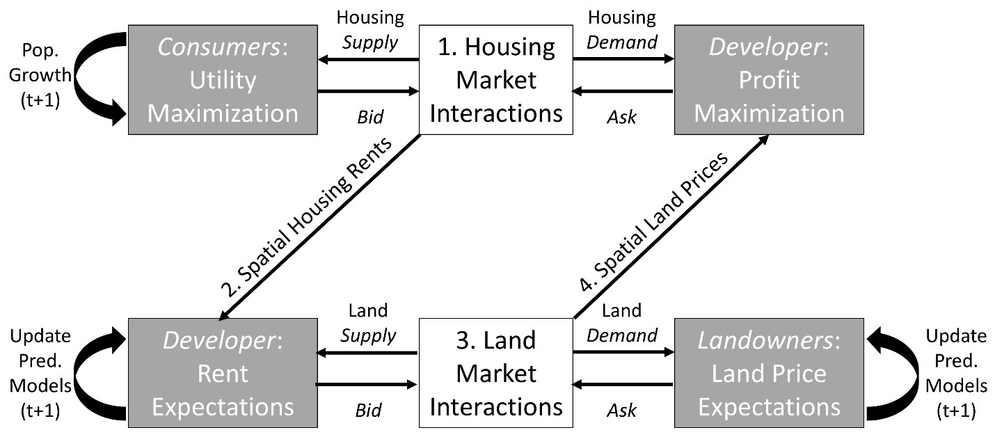
The ABM presented here is a version of the CHALMS model (Magliocca et al. 2011, 2012) adapted to a coastal landscape. The model simulates the conversion of undeveloped land to residential housing through spatial and utility- or profit-maximizing decisions by residential housing consumers, a representative developer, and landowners (Figure 1). A full model description using the Overview, Design concepts, and Details + Decision-Making (ODD+D; Grimm et al. 2010; Müller et al. 2013) is provided as a supplemental document. The main objective of the original version of CHALMS is to understand which landscape features and agent interactions are most important for explaining the timing and location of residential housing development. In the coastal version presented here, the influence of coastal amenities and risk of property damage from storms is also considered. To do this, CHALMS explicitly links housing and land markets to simulate endogenous, coupled market prices. Understanding spatially explicit and time-varying dynamics that result from land and housing market interactions is essential for evaluating potential outcomes of land-use policies (e.g., zoning; Magliocca et al. 2012).
Landscape and model initialization
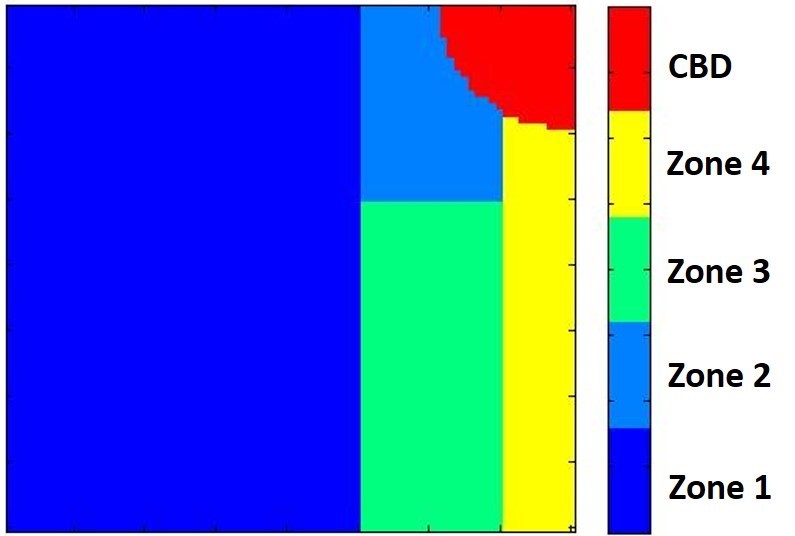
The simulated landscape is a stylized representation of a developing coastal region, i.e., does not represent any particular geographic area. Land acquisition and, in part, residential location decisions are based on two landscape attributes: distance to a central business district (CBD), which influences travel costs to places of employment, and proximity to the coastline from which consumers derive utility in the form of a natural amenity (Figure 2). Potential damages from storm impacts are also related to proximity to the coast (decreasing with distance from the coast) and the annual probability of storm occurrence. Travel costs increase linearly with distance from the CBD at a rate of $25.85 per cell (based on annual travel assumptions, see Magliocca et al. (2011 for details). Natural amenities related to proximity to the coast (Benson et al. 1998; Bourassa et al. 2004; Bin et al. 2008) decay nonlinearly as distance from the coast increases (Figure 2). Spatially-varying expected costs associated with property damages from coastal storms are a function of both proximity to the coast (Figure 2) and the annual probability of storm occurrence (Costanza et al. 2008). The model is executed for 20 discrete time steps (one model time step equals a year) over a gridded cellular landscape of 6,400 cells (80 by 80) and each cell is equivalent to one acre. The simulation time span was chosen based on the assumption that the development process would experience minimal fundamental changes over 20 years (e.g., from financing innovations), and the spatial extent was chosen to minimize any spatial boundary effects on development given the simulation time span. For the exception of the selected experimental parameters, all sources of stochasticity (e.g., assignment of agents’ price prediction models, learning time horizon, income) are held constant using a random number seed.
The model is initialized with a developed CBD that contains a mix of housing types on lots of either 0.25, 0.5, 1, or 2 acres and house sizes of 1,500 or 2,500 square feet (Figure 2). All new houses that are built over the course of model execution are a combination of one of these existing house and lot sizes (i.e., no new housing types are introduced). At the beginning of the simulation, the same number of consumers are initialized as there are number of houses in the CBD. Consumers are heterogeneous in their incomes and preferences for house size, lot size, and proximity to the coast. Consumer incomes and housing and location preferences are randomly drawn from uniform distributions. Undeveloped land is subdivided into 64 100-acre parcels (10 by 10 cells) that are regularly distributed across the landscape (Figure 2). Each undeveloped parcel is assigned to a single landowner agent.

Agent decision-making processes
The formalization of agent decisions and market transactions are identical to those in the original CHALMS framework and described in detail in Magliocca et al. (2011). Developer and landowner agents form expectations of future land prices in the land market based on observed prices in the past and relative location in the landscape (see Agent Prediction in ODD). Land market transactions are based on the bilateral transaction framework developed by Filatova et al. (2009). The developer forms a bid price for each undeveloped parcel based on spatially explicit expected rents for housing, and landowners form asking prices based on their expected value of the land in its most profitable use (e.g., agriculture versus residential housing). If the developer’s bid price is higher than the landowner’s asking price, then a transaction occurs and the entire parcel transfers ownership.
Given observed land purchase prices, the developer ranks each housing type from highest to lowest expected return (i.e., expected rents net of construction and land costs) given distance to the CBD and coast in every owned and/or undeveloped cell in existing land holdings or newly acquired parcels. The housing type with the highest expected return in a given cell is built first, with others following in remaining owned and undeveloped cells in the order of descending expected returns. Housing construction of a given type continues until as many houses of that type are built as the developer expects will be demanded by consumers, or all vacant land is developed. New houses are assigned the closet distance from the CBD and highest coastal amenity value of any cell in the new lot’s footprint. New and existing vacant houses are then offered for sale in the housing market with an asking price equal to the developer’s expected rent for the given housing type and location.
New housing consumers are introduced into the ‘consumer pool’ of existing consumers at the start of each time step at a rate of ten percent a year. Each consumer c generates utility from housing and a composite non-housing good, x. Each house i is characterized by its size, hi, its lot size, li, and an amenity that is a function of the distance from the coast, a(di), where di is house i’s distance from the coast. We assume that the utility function has a standard Cobb-Douglas structure:
| $$U(i,c)=x^{\alpha_c} h_i^{\beta_c} l_i^{\gamma_c} a(d_i)^{\delta_c}\text{; s.t.:}\,\alpha_c+\beta_c+\gamma_c+\delta_c=1$$ | (1) |
A consumer has income, I, pays (annualized) price, Pi, for house i, and pays travel costs, \(\psi_i\), which depend on house i’s distance from the central business district (CBD). Consumers also face an annual probability, \(\rho\), of property damage from coastal storms [1]. When a storm occurs, it imposes a cost, which we assume is a percentage of the house’s value. The percentage varies with the house’s distance from the coast, \(C(d_i)\); where \(\frac{\delta C_i}{\delta d_i}<0\) Thus, the budget constraint is given by:
| $$I=x+P_i(1+\rho C(d_i))+\psi_i$$ | (2) |
In this version of the model, we assume that consumers know the probability of a storm and the costs they will incur if a storm takes place. We also abstract from considerations of insurance. Both assumptions will be relaxed as a focus of future research.
Consumers place bids on all houses that generate positive utility and are thus within their budget constraints given asking prices. Each consumer observes the number of other consumers placing bids on their set of prospective houses and adjusts their bid according to competition levels. If there are more bids than there are houses being bid on, then bid prices are adjusted upwards. If there are fewer bids than there are houses being bid on, then bid prices are adjusted downwards. Bid adjustments are designed to reflect the relative supply of and demand for housing and quantify competition with the housing market. Houses are assigned to consumers with the highest bids for each house. If a consumer has the winning bid on multiple houses, then the consumer chooses the house that generates the highest utility given the winning bid prices. Consumers that locate in a house are assigned a residence time drawn randomly from a normal distribution (\(\mu=12.5\), \(\sigma=11\) time steps). When residence time is exceeded, the consumer moves-out, re-enters the consumer pool, and the newly vacant house is put back on the market. Consumers that do not locate after three consecutive time steps are removed from the consumer pool.
Space- and Time-Varying Global Sensitivity Analysis
The overall objective of the following GSA model experiments is to elucidate the extent to which parameters and their interactions contribute to variability in model outcomes. These experiments do not to establish causality between any particular parameter and development patterns in any particular location or single model realization. The intent is to illustrate the utility of combining variance- and density-based GSA approaches, rather than to draw conclusions about any particular coastal systems.
Variance-based GSA
Variance-based GSA decomposes the variance (V) of a selected model output (Y) from the perturbations of k=7 model inputs (Table 1) into the contributions of single (Vi) and combinations of model inputs with increasing dimensionality (Ligmann-Zielinska and Sun 2010):
| $$V=\sum_i V_i+\sum_{i<j}V_{ij}+\sum_{i<j<m}V_{ijm}+\dots +V_{1:k}$$ | (3) |
| $$S_i=\frac{v_i}{v}=\frac{v_{X_i}[E_{X_{-i}}(Y|X_i)]}{V(Y)}$$ | (4) |
| $$ST_i=\frac{V(Y)-V_{X_{-i}}[E_{X_i}(Y|X_{-i})]}{V(y)}=S_i+S_{ij}+S_{im}+S_{ijm}+\dots+S_{i:k}$$ | (5) |
The proportion of model output variance (V) attributed to input i independent of other inputs (k-1) is given by Si, and STi describes the overall contribution of input i and its interactions with other inputs to the overall model output variance (Ligmann-Zielinska and Sun 2010, Saltelli et al. 2010). The contributions to variance in model output Y of all inputs other than i is represented by the expression \(V_{X_i}[E_{X_{-i}}(|X_i)]\).
| Input | Description | Statistics | |
| Storm Frequency (Mf) | Probability of a coastal storm of a fixed severity occurring in any given year. | D | (0.0065, 0.7143) |
| Storm Severity (Ms) | Intercept of distance from coast damage function in Figure 2 in units of percent of property value. | N | (10, 5) |
| Coastal Amenity (Ao) | Utility derived from coastal amenity. | N | (500,000, 125,000) |
| Amenity Decay Rate (r) | Rate of decline in coastal amenity value with distance from the coast. | N | (0.1, 0.05) |
| Heterogeneity Among Amenity Preferences (δc) | Range of consumer preference for coastal amenity. Maximum of range is specified. | U | (0.9, 0.1) |
| Travel Costs (ψi) | Cost per mile traveled to CBD. | N | (1.30, 0.65) |
| Discount Rate (R) | Economic discount rate used to annualize land and housing prices. | N | (0.05, 0.025) |
We follow the time-varying GSA method developed by Ligmann-Zielinska and Sun (2010), which is based on the quasi-random Sobol estimation procedure (Saltelli 2002; Lilburne and Tarantola 2009) and implemented using a sequential estimation algorithm in Matlab developed by Tarantola (2013). In addition, building on the approaches by Hall et al. (2005), Lilburne and Tarantola (2009), and Ligmann-Zielinska et al. (2014b), spatially distributed sources of sensitivity are investigated at the regional (aggregate) scale as well as in several representative sub-regions within the landscape (fine-scale). For time-GSA, Si and STi are calculated for every time step to determine to what extent particular parameters are stronger or weaker drivers of model outcomes over time. For space-GSA, the landscape is divided into five ‘zones’ (i.e., sub-regions) based on their perceived value for development relative to their proximity to the coast (Figure 3). In preliminary experimentation, each zone showed internally consistent yet distinct development dynamics from other landscape regions. The CBD is excluded from analysis because the selected model outputs – number of houses built, percent developed area, and diversity of the housing stock – remain constant over the course of model execution in that location.
Density-based GSA
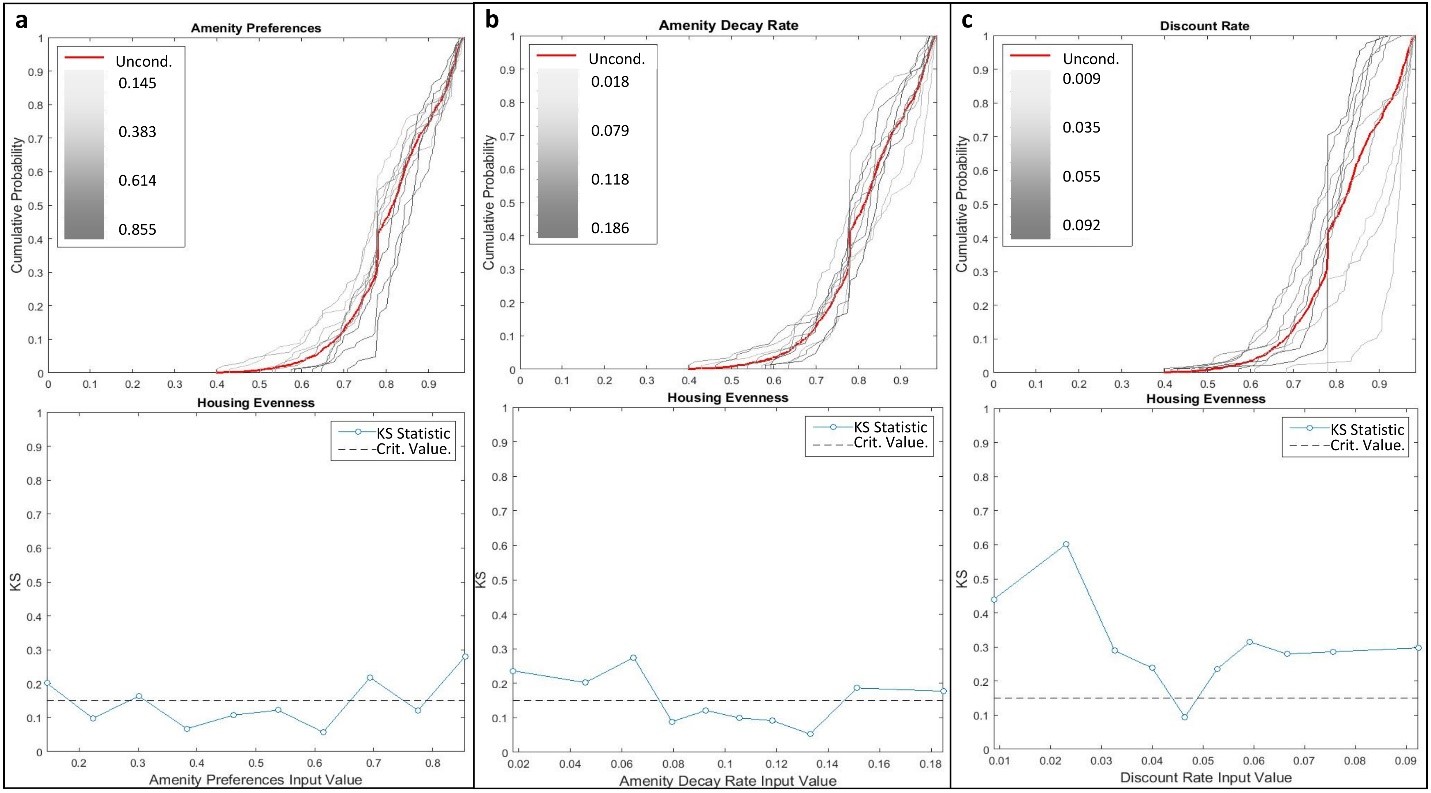
The density-based GSA approach developed by Pianosi and Wagener (2015), PAWN, is both methodologically and conceptually complementary to the variance-based GSA methods. PAWN is based on the comparison of conditional and unconditional CDFs of model output. The unconditional CDF is simply the distribution of model outputs generated from all parameter values used in the Sobol estimation procedure for the variance-based GSA. The conditional CDF is generated by fixing the value of one input parameter while letting other parameter values vary. Fortunately, this approach can be applied to existing datasets (i.e., using the same simulation data for both variance- and density-based analyses) by grouping model executions with similar input parameter values, which can then be treated as ‘fixed’ value sub-sets from the parameter distribution (Pianosi and Wagener 2015). Conditional distributions account for changes in outcome distribution when variability from a particular parameter (or parameter group) is removed, and thus the distance between the conditional and unconditional distributions is a measure of output sensitivity. The significance of the distance between conditional and unconditional distributions is tested with the Kolmogorov-Smirnov (KS) statistic (Kolmogorov 1933; Smirnov 1939).
Fixed groups are specified here by sub-setting each input parameter distribution generated by the quasi-random Sobol estimation procedure into ten equal-frequency quantiles, and thus the ‘fixed’ value for each quantile group is the median of the quantile. Conditional CDFs are then created by removing one parameter group at a time to observe the effect on model outcome distributions. All conditional CDFs are then plotted against the unconditional CDF and the KS statistic is calculated for each fixed value and compared against the critical value of the KS statistic at confidence level of 0.05. KS statistic values exceeding the critical value indicate a statistically significant influence of the parameter at the given fixed value. Importantly, this analysis is applied only to final model outcomes, as no spatial or temporal details about parameter sensitivities are provided. Thus, PAWN is a complement to variance-based in that it provides insight into where in parameter distributions sensitivities in model outcomes are produced.
Experimental approach
A key consideration when conducting GSA is the number of model executions required to obtain accurate sensitivity estimations. Estimations of sensitivity indices Si and STi are calculated from a number of base samples (N), which each contain k + 2 quasi-random parameter samples used for sequential estimation, and bring the total number of model executions required to N(k + 2) (Tarantola 2013). The larger the N, the more precise the sensitivity estimates, but practically the selection of N depends on the computational cost of the model. Relatively inexpensive models can have an N in excess of 500, but more expensive models may have an N on the order of 30-100 (Tang et al. 2006). Additionally, as the complexity and nonlinearity of a given model increases, so too should N. For this study, an N = 100 is selected for a total of 900 model executions as a compromise between estimation accuracy and computational demand. A single model execution using the parallel computing toolbox in Matlab requires roughly 90 minutes run-time, which results in a total of 1,350 hours of run-time on a multi-threaded 3.20 GHz AMD Opteron™ Processor 6328.
Input parameter distributions
Seven independent model input parameters are used (Table 1): storm frequency, storm severity, maximum natural amenity value at the coast (Ao; Figure 2), rate of coastal amenity decrease with distance from the coast (r; Figure 2), range of consumer preference for coastal amenity (\(\delta_c\), Equation 1), travel costs to CBD (\(\psi_i\), Equation 1), and economic discount rate. The economic discount rate is used by the developer to calculate the profitability and formulate future asking prices of particular housing types given observed housing and land prices. Table 1 describes the probability density functions (PDFs) used for quasi-random sampling.
For all normally distributed inputs we assume a standard deviation of half the mean to ensure sufficient perturbations of parameter values. Probabilities of storm occurrence (Mf) are aggregated from Costanza et al. (2008) across all storm severity categories for the Atlantic coast to estimate discrete annual probabilities of storm occurrence of any severity. Storm severity (Ms) is varied independently by modifying percent loss of property value (Figure 2). Storm frequency and severity are decoupled in this way for use with an expected cost framework for resolving consumer location decisions. Consumer preferences for coastal amenities (\(\delta_c\), Equation 1) are randomly drawn from a uniform distribution of varying range. For the purposes of exploring model output sensitivities to this formalization, the quasi-random sampling procedure is applied to the maximum of the preference distribution (e.g. [0.1, 0.9] vs. [0.1, 0.5]) to explore the effects of a more or less heterogeneous and strong preference for coastal amenities among the consumer agent population.
Output parameter selection
Three model outputs are selected for sensitivity analyses: number of houses, percent developed area, and diversity of the housing stock. The first two outputs relate mainly to spatial patterns of development and provide measures of the cumulative effects of household location decisions over time. The diversity of the housing stock, or housing stock evenness, at each period is measured using Shannon’s entropy. This index describes the relative likelihood of a particular house type being built in a given period. In other words, as the distribution of housing types in the overall housing stock becomes more even (Shannon entropy approaches 1), each housing type is equally likely as any other to be built and housing offerings are essentially random. Conversely, as the distribution of housing types in the overall housing stock becomes more uneven (Shannon entropy approached 0), a particular housing type (or set of housing types) is more likely to be offered reflecting relatively more desirable and/or profitable housing types. Such a measure can be related to self-reinforcing and/or path-dependent processes in the development process.
Results
The complete set of model outputs included temporally and spatially explicit land-use maps giving the locations, types, and prices of housing, consumer preferences and incomes, and transaction prices for land. Selected model outputs were aggregated within each of the sub-regional ‘zones’ (Figure 3) and sensitivity indices were calculated every time step for each zone. Figure 4 shows an example of variation in development patterns with low and high coastal amenity decay rates (r) for two selected model executions. Note that a perturbation in only this input parameter resulted in large variation in the location of development.

Sequential sensitivity estimation errors
The accuracy of sensitivity indices depends on the selection of N (Saltelli et al. 2008), however the optimum N is often not known a priori for complex models. Using the quasi-random Sobol sampling method and algorithm for sequential estimation of sensitivity indices developed by Tarantola (2013), the root means squared error (RMSE) of first-order sensitivity was calculated for each model execution to track convergence of sensitivity estimates to a moving average for each selected model output (Figure 5). Given the computation expense of the coastal CHALMS model, RMSE values below 15 percent (RMSE = 0.15) were deemed satisfactory (Saltelli et al. 2008). RMSE values for the number of houses built and percent developed area (Figure 5a and 5b) for all input parameters were generally less than the threshold for all model executions, except for slight increases in variability due to discount rate. In the case of housing stock evenness (Figure 5c), variability due to storm frequency and discount rate were above the RMSE threshold by the final model execution. However, RMSE values were relatively stable, fluctuating around their overall mean values through all model executions. Hence, N=100 samples were sufficient to conduct both GSAs on these model outputs.

Spatial and temporal GSA
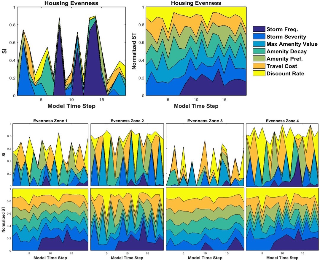
For variance-based GSA, time-dependent first-order (Si) and total effect (STi) sensitivity indices are plotted cumulatively at the regional and zonal levels for each selected model output. These are paired with outcome variance from density-based GSA presented as CDF and KS statistic plots of regional outputs from input parameters. For interpretation of variance-based sensitivity indicators, the effects of model inputs are additive when interactions are linear and the sum of Si nears 1 (Ligmann-Zielinska and Sun 2010). As non-additive behavior increases, the proportion of variance attributed to interactions among parameters increases, the sum of Si decreases, and areas plotted as white in Si plots increase. Regionally, variance in houses built and percent developed area was mostly additive, while variance in housing stock evenness was mostly due to parameter interactions. For all outputs, no single input parameter was consistently influential over time, as sensitivity indices oscillated frequently as the development process unfolded. Furthermore, sensitivity profiles at the zonal level were quite different from one another and regional profiles, which emphasized the importance of studying spatial as well as temporal global sensitivity.
Number of houses built
At the regional level, storm frequency (Mf) was responsible for much of the variance (Si) observed in the number of houses built (Figure 6) after seventh model time step. On average, amenity preference (\(\delta_c\)), travel costs (\(\psi_i\)), and discount rate (R) accounted for an average of 50% of total variance (STi) when interacting with other factors. Closer inspection with density-based GSA shows that outcome variance from storm frequency at the regional level is driven exclusively by the highest probability storm climate (Figure 7a). Additionally, the discount rate consistently influenced the number of houses built, with high and low discount rates and moderate discount rates tending to lead to fewer and more houses than the global average, respectively (Figure 7b).

Zonal sensitivities were quite different than those at the regional level. Discount rate (R) and travel costs (\(\psi_i\)) were almost entirely responsible for variance in the number of houses built in zone 1. Storm frequency was not influential in any zone, whereas the other input factors alternated in importance over time. Inputs amenity preference, amenity decay rate, travel costs, and discount rate are all influential factors in consumers’ decisions to locate in proximity to either the CBD or coast, as well as interacting strongly to drive housing and land prices. For example, competition for coastal property in zone 4 may have pushed consumers inland and driven development in zone 1.
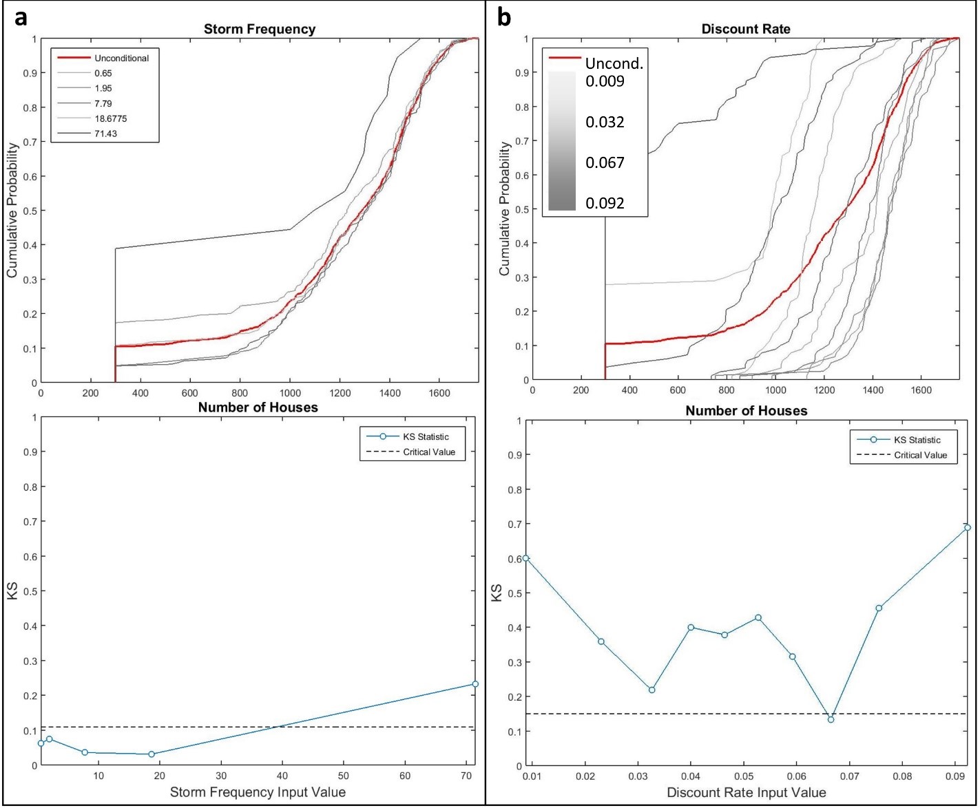
Percent developed area
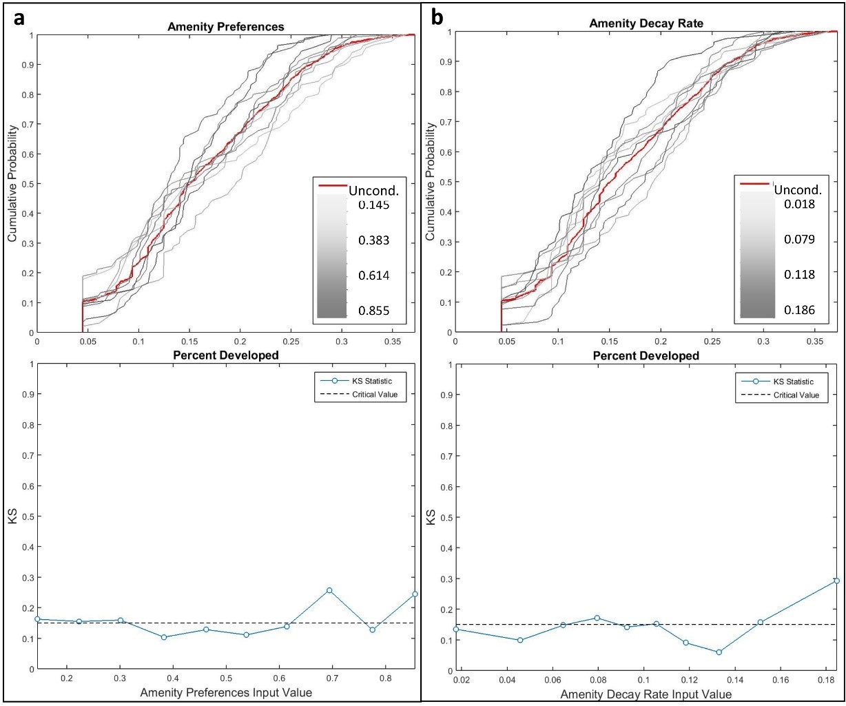
At the regional level, storm frequency was responsible for much of the variance observed in the percent of developed area (Figure 8) after seventh model time step. Just as for the number of houses built, density-based GSA revealed that the highest storm frequency was mostly responsible for regional variance. Less area developed on average with high and low discount rates, while moderate discount rates lead to more developed area than the global average. Figure 9a and Figure 9b also show that higher values of amenity preference and decay rate influenced the percent developed area, with increased preferences for amenities and faster decay of amenity values led to less developed area overall. However, because the relative differences between STi and Si were large at various time steps for model inputs other than storm frequency, we conclude that all contributed significantly to overall variance through their interactions with other model parameters (i.e., non-additive; Ligmann-Zielinska and Sun 2010).

Zonal sensitivities were quite different from those at the regional level, as no single model input was consistently important over time across all zones. All zones exhibited cyclical patterns of influence on variance with one or two parameters dominating in any single time step. In general, travel costs and discount rate consistently accounted for 20% to 40% of variance, while amenity- and storm-related decreased and increased in importance, respectively, moving from inland to coastal zones. Unlike the number of houses, storm frequency remained important at the zonal level for the percent developed area. This suggests that increased storm frequency tends to modify the density of housing, because variance in developed area is high and the number of houses is comparatively insensitive to storm frequency changes.
Housing stock evenness
Sensitivity of housing stock evenness was mainly driven by interactions among inputs at both regional and zonal levels (Figure 10). The sum of Si values averaged 50% throughout model execution at the regional level. Similarly, STi values were relatively evenly distributed among all of the model inputs further reinforcing the importance of input interactions for housing stock outcomes. Density-based GSA was particularly revealing in this context. Higher amenity preference and lower amenity decay rate values tended to create more even housing stocks (Figure 11a and Figure 11b). Both of these conditions provide more overall amenity value across the landscape, which mediated the effects of income and location differences that tend to favor some housing types over others. For example, ceterus paribus, higher income consumers tend to preferentially occupy houses on larger lots, and high density housing tends to occur in close proximity to the coast due to higher profit margins. Discount rates also demonstrated directional influences of housing stock evenness, with lower rates leading to more even housing stock (Figure 11c).
Discussion
Space- and time-varying GSA revealed input parameter interactions differed over both time and spatial scales and across selected model outputs. For the exception of housing stock evenness, the sum of first-order effects at the regional scale ranged from 70% to 100%, meaning that a high proportion of output variance at that scale was additive. However, there were instances in particular zones and at various points during model execution that the sum of first-order effects dropped to 20-40% across all model outputs, indicating the importance of localized spatial interactions in the development process. For example, storm frequency was highly interactive with other inputs in non-coastal zones, specifically in Figures 8 and Figure 10, which could be indicative of spatial ‘spill-over’ effects from high land and/or housing prices in the coastal area (Irwin and Bockstael 2002). In other words, market dynamics in one part of the landscape influenced development in adjacent areas of the landscape, i.e., ‘spill-over’.
Furthermore, input interactions over time were apparent in the cyclical patterns of variance observed at both regional and zonal levels. Cyclical patterns were observed in total-effect indices for all regional level outputs as inputs alternated in importance of driving output variance over time. Two intrinsic features of the model that reflect land and housing markets characteristics explain the emergence of these patterns. Land markets have been described as “thin markets” (Irwin and Wrenn 2014), meaning market transactions occur at relatively low frequency and are geographically dispersed, as opposed to other markets (e.g., financial) which tend to have many more transactions and more continuous price dynamics as a result. Additionally, the discrete nature of land parcels and housing options over which agents make decisions create discontinuous land and housing market dynamics. Such cyclical behavior is often attributed to delayed feedbacks created by a time lag between a change and the effects of that change on the rest of the system (Manson 2007). This form of complexity is important to represent in ABMs, particularly when investigating spatially-explicit interactions that operate unevenly over time across the landscape. The relative regularity of the cyclic patterns is explained by the constant, imposed rate of population growth and fixed landowner parcel sizes. In other words, demand for land and amount of land purchased to meet that demand were relatively steady over time, which produced a consistent (although not deterministic) cyclic structure in model sensitivity. Time-varying GSA enabled the detection of these interactions via their effects on output variation.
Sensitivities of housing stock evenness, in particular, illustrated the highly complex and nonlinear nature of market processes. Housing stock diversity results from many short timescale feedbacks between structural features of land and housing markets (e.g., transaction costs, construction costs) and behavioral features of landowners, developers, and housing consumers (e.g., price expectations, location preferences, risk tolerances). Sensitivity indices showed that the majority of variance in housing stock diversity was due to interactions among input parameters and model features (Figure 10). Application of conventional OAT approaches to sensitivity analysis would not have detected the importance of input interactions in such emergent phenomenon, and may have even generated misleading conclusions about the magnitude and relative importance of housing stock evenness sensitivity to particular input parameters.
The relatively large differences in sensitivities across zones, coupled with evidence of the importance of interactions for explaining variance, suggest that housing stock diversity is potentially a locally path-dependent and regionally state-dependent phenomenon. Page (2006, p. 95) defines a state-dependent process as one in which the outcome at any time depends only of the state of that processes at a given time, and different states that lead to the same future state are equivalent. In this context, the relative proportion of different housing types present in the overall housing stock at any given time, described here as the evenness of the housing stock using Shannon entropy, can be considered the housing stock state. A path-dependent process is one in which the outcome at any time depends on both past states and their order of occurrence (Page 2006, p. 97). At the zonal level, housing stock evenness was generally the result of path-dependent processes. Local spatial interactions and market forces made it more likely that a particular housing type would be built in each zone if it had been built there previously (Figure 12). In contrast, regional level housing stock evenness tended to become more even over time, suggesting that regional housing stock diversity was the result of state-dependent processes. Feedbacks from the regional land and housing markets stabilized overall housing diversity over time and ensured that roughly similar housing stocks consistently emerged at the regional level regardless of the order in which particular housing types were built in different locations. Such complex, cross-scale dynamics would not have been detectable with conventional sensitivity analyses.
While space- and time-varying GSA is an appropriate analytical tool for complex ABMs, its application presents a number of conceptual and computational challenges that conventional methods do not. The number of model executions required for GSA can be exponentially higher than for convention methods. Sufficient sample size is critical to producing accurate estimates, with more uncertain outputs potentially requiring (many) more than other outputs. Given the computational expense, the analyst is faced with a trade-off between extended processing time and estimation accuracy. Sequential estimation techniques, such as the Sobol method used here (Tarantola 2013), have the potential to optimize the number of model executions performed (Tang et al. 2006). However, this method prohibits parallel model executions, which can lead to exorbitant run times for computationally expensive models. Here, we selected a large number of initial base samples based on the literature (Tang et al. 2006; Ligmann-Zielinska and Sun 2010; Tarantola 2013), generated quasi-random parameter samples beforehand, executed each model run in parallel, and evaluated convergence of sensitivity estimates post-hoc (section 4.1). This approach required 1,350 hours of run-time as opposed to approximately 9,000 hours that would have been required if model execution had been performed in sequence.
One of the benefits of GSA is the identification of uncertain input parameters that contribute insignificantly to output variance, and thus can be fixed without changing overall model output (Ligmann-Zielinska and Sun 2010; Ligmann-Zielinska et al. 2014b). However, as this analysis demonstrated, in highly nonlinear ABMs, it may not be possible to identify and fix such parameters because of their highly interactive nature. If particular parameters can be specified empirically, such as travel costs and discount rate, this may eliminate sources of uncertainty even though the model is sensitive to these parameters. In contrast, some input parameters to which the model is highly sensitive, such as the spatial distribution of amenity values and consumers’ location preferences for coastal amenities, are likely to be heterogeneous across consumers and difficult to estimate empirically. In such cases, GSA is a useful tool for describing model sensitivities even if it does not ultimately lead to reducing model sensitivities through parameter fixing. In either case, GSA can identify parameters responsible for significant output variance, which then become priorities for data collection when developing an empirically parameterized model.
Conclusions
Although the CHALMS model is initialized with stylized parameter values and landscape configuration, this application of combined variance- and density-based GSA highlighted issues that apply to both theoretically- and empirically-based spatial ABMs. Variance-based GSA can be extremely computationally expensive, particularly when model outcomes are highly uncertain and require thousands of model executions to obtain accurate sensitivity estimates. As we demonstrated here, an iterative process in which quasi-random input parameters are generated a priori, model executions are performed in parallel, and estimation error is calculated post-hoc is a promising alternative to sequential model execution and sensitivity estimation for models with equally or more complex behavior than CHALMS. Density-based GSA using PAWN (Pianosi and Wagener 2015) also provides insight into the magnitude and directionality of model sensitivities, and it can be applied to existing model data, eliminating the need for additional model executions.
The computational cost of GSA methods for complex models is daunting but necessary. Once a model is capable of producing nonlinear and adaptive behaviors, such as path-dependent development patterns, a threshold is passed beyond which model outcome variability, and therefore the number of model executions required for GSA, is not reducible (Brown et al. 2005; Manson 2007). Such a gradual approach is both pragmatic, given the computational demands required, as well as necessary in order to implement comprehensive sensitivity analysis of complex ABMs.
Spatially and temporally explicit variance-based GSA and complementary density-based GSA have the potential to deepen understanding of the sensitivities of complex, dynamic ABMs. Uncertainty in input parameters contributes not only to sensitivity of model outcomes, but also to spatially- and temporally-varying sensitivities in model dynamics. One of the main advantages of ABMs over other top-down modeling or statistical approaches, particularly for studying land-use change, is to explicitly model the time path, or evolution, of emergent phenomenon. However, interpretation of results remains more challenging than for conventional methods, especially when ABMs possess many nonlinear characteristics, such as path-dependence (Brown et al. 2005; Manson 2007). This emphasizes the need for parsimony in model design. Even simple models can produce complex behavior (Sun et al. 2016), but the task of GSA is made easier and more efficient if the number of uncertain parameters (or overall number of parameters) can be reduced.
The ABM research community is engaged in an ongoing debate about the most appropriate SA methods. Specifically, Saltelli et al. (2008) and Ligmann-Zielinska et al. (2014b) have concluded that variance-based GSA is the most appropriate method for process-based models characterized by parameter interactions and emergence. Conversely, ten Broeke et al. (2016), recommend OAT over regression-based and GSA methods, because, they argue, these other methods consider only averaged parameter effects, masking nonlinear model mechanics. In light of our findings here, we agree with ten Broeke et al. on this point. Variance- and density-based GSA methods used alone are not sufficient for understanding model mechanics, because they fail to address either the directionality or dynamics of parameter effects on model outcomes, respectively. However, also clear from our findings is that accounting for parameter interactions is essential for understanding and quantifying the full scope of model behavior driven by uncertain parameters. Because OAT methods do not consider interaction effects, they will always be limited to partial examinations of model outcome space. Emergent model behaviors resulting from unique, simultaneous combinations of two or more parameters cannot be captured by perturbing one parameter at a time. Only global approaches that consider the full range of all uncertain parameters within a single analysis can rigorously investigate such behaviors. Furthermore, we have demonstrated that pairing complementary GSA methods can address the remaining criticisms of GSA methods. Specifically, density-based GSA can reveal which parts of individual parameter distributions are associated with model output sensitivities, and how robust model outcomes are to various parameter combinations within and across multiple parameter distributions (i.e., hotspots within the global parameter space). The prevalence (or sometimes dominance) of parameter interactions in ABMs requires the comprehensiveness that GSA methods provide, and restricts OAT methods to a useful means of model exploration.
The unique combination of GSA methods implemented here enriched our understanding of how our assumptions about parameters values affected modeled dynamics. Highly sensitive model outputs were identified for future model experiments in which the sampling space will be refined, and data collection efforts will be targeted to constrain parameters that produce model sensitivity. Critical sources of model sensitivities were also identified across space and over time that lead to new research questions. For example, the influence of storm frequency was stronger in certain locations and at different times during simulation runs. This leads to the question: how does the timing of storms – earlier or later in simulations, which impact less or more developed area, respectively – affect development dynamics? Ultimately, these are the types of questions that comprehensive GSA can raise, and force us as modelers to deepen our understanding of complexity in land-use ABMs.
Acknowledgements
The authors were supported by funding received from the National Science Foundation, Grant #1331399 EAR – SEES Hazards.Notes
- For simplicity, we assume only one type of storm with a fixed severity. Storm severity is altered as part of the sensitivity experiment.
References
AVISSAR, R. (1995). Scaling of land–atmosphere interactions: an atmosphere modelling perspective. Hydrological Processes, 9(5-6), 679–695. [doi:10.1002/hyp.3360090514]
BARONI, G., & Tarantola, S. (2014). A general probabilistic framework for uncertainty and global sensitivity analysis of deterministic models: a hydrological case study. Environmental Modelling & Software 51, 26-34.
BENSON, E.D., Hansen, J.L., Schwartz Jr, A.L., & Smersh, G.T. (1998). Pricing residential amenities: The value of a view. The Journal of Real Estate Finance and Economics, 16(1), 55-73. [doi:10.1023/A:1007785315925]
BIN, O., Crawford, T.W., Kruse, J.B., & Landry, C.E. (2008). Viewscapes and flood hazard: Coastal housing market response to amenities and risk. Land Economics, 84(3), 434-448.
BOURASSA, S. C., Hoesli, M., & Sun, J. (2004). What's in a view? Environment and Planning A, 36(8), 1427-1450. [doi:10.1068/a36103]
BROWN, D.G., Page, S., Riolo, R., Zellner, M., & Rand, W. (2005). Path dependence and the validation of agent-based spatial models of land use. International Journal of Geographical Information Science, 19(2), 153-174.
BRUGNACH, M. (2005). Process level sensitivity analysis for complex ecological models. Ecological Modeling, 187(2), 99-120. [doi:10.1016/j.ecolmodel.2005.01.044]
CARIBONI, J., Gatelli, D., Liska, R., & Saltelli, A. (2005). The role of sensitivity analysis in ecological modeling. Ecological Modeling, 203(1), 167-182.
COSTANZA, R., Pérez-Maqueo, O., Martinez, M.L., Sutton, P., Anderson, S.J., & Mulder, K., 2008. The value of coastal wetlands for hurricane protection. AMBIO, 37(4), 241-248. [doi:10.1579/0044-7447(2008)37[241:TVOCWF]2.0.CO;2]
DUBUS, I.G. & Brown, C.D. (2002). Sensitivity and first step uncertainty analyses for the preferential flow model MACRO. Journal of Environmental Quality, 31(1), 227–240.
FILATOVA, T. & Bin, O. (2014). 'Changing Climate, Changing Behavior: Adaptive Economic Behavior and Housing Markets Responses to Flood Risks.' In B. Kaminski & G. Koloch (Eds.), Advances in Social Simulation: Proceedings of the 9th Conference of the European Social Simulation Association. Berlin Heidelberg: Springer, pp. 249-258. [doi:10.1007/978-3-642-39829-2_22]
FILATOVA, T., Parker, D.C., & van derVeen, A. (2009). Agent-based urban land markets: Agent’s pricing behavior, land prices and urban land use change. Journal of Artificial Societies and Social Simulation 12(1), 3: https://www.jasss.org/12/1/3.html.
FILATOVA, T., Parker, D.C., & van derVeen, A. (2011). The implications of skewed risk perception for a Dutch coastal land market: Insights from an agent-based computational economics model. Agricultural and Resource Economics Review, 40(3), 405-423. [doi:10.1017/S1068280500002860]
GRIMM, V., Berger, U., DeAngelis, D. L., Polhill, J. G., Giske, J., & Railsback, S. F. (2010). The ODD protocol: a review and first update. Ecological modelling, 221(23), 2760-2768.
HALL, J.W., Tarantola, S., Bates, P.D., & Horrit, M.S. (2005). Distributed sensitivity analysis of flood inundation model calibration. Journal of Hydraulic Engineering, 131(2), 117–126. [doi:10.1061/(ASCE)0733-9429(2005)131:2(117)]
HUANG, Q., Parker, D.C., Filatova, T., & Sun, S. (2014). A review of urban residential choice models using agent-based modeling. Environment and Planning B: Planning and Design, 40, 000-000.
IRWIN, E.G. & Bockstael, N.E. (2002). Interacting agents, spatial externalities and the evolution of residential land use patterns. Journal of Economic Geography, 2(1), 31-54. [doi:10.1093/jeg/2.1.31]
IRWIN, E.G., Jayaprakash, C., & Munroe, D.K. (2009). Towards a comprehensive framework for modeling urban spatial dynamics. Landscape Ecology, 24(9), 1223-1236.
IRWIN, E.G. & Wrenn, D.H. (2014). 'An assessment of empirical methods for modeling land use.' In J. M. Duke & J. Wu (Eds.), The Oxford Handbook of Land Economics. Oxford: Oxford University Press.
KOLMOGOROV, A. (1933). Sulla determinazione empirica di una legge di distribuzione. Giornale dell’Istituto Italiano degli Attuari, 4, 83-91.
LIGMANN-ZIELINSKA, A. & Sun, L. (2010). Applying time-dependent variance-based global sensitivity analysis to represent the dynamics of an agent-based model of land use change. International Journal of Geographical Information Science, 24(12), 1829-1850. [doi:10.1080/13658816.2010.490533]
LIGMANN-ZIELINSKA, A. (2013). Spatially-explicit sensitivity analysis of an agent-based model of land use change. International Journal of Geographical Information Science, 27(9), 1764-1781.
LIGMANN-ZIELINSKA, A., Liu, W., Kramer, D.B., Cheruvelil, K.S., Soranno, P.A., Jankowski, P., & Salap, S. (2014a). Multiscale spatial sensitivity analysis for agent-based modelling of coupled landscape and aquatic systems. Proceedings of the International Environmental Modelling and Software Society (iEMSs) International Environmental Modelling and Software Society. http://www.iemss.org/society/index.php/iemss-2014-proceedings.
LIGMANN-ZIELINSKA, A., Kramer, D. B., Cheruvelil, K. S., & Soranno, P. A. (2014b). Using Uncertainty and Sensitivity Analyses in Socioecological Agent-Based Models to Improve Their Analytical Performance and Policy Relevance. PloS One, 9(10), e109779.
LILBURNE, L.R., Webb, T.H., & Francis, G.S. (2003). Relative effect of climate, soil, and management of nitrate leaching under wheat production in Canterbury, New Zealand. Australian Journal of Soil Research, 41(4), 699–709. [doi:10.1071/SR02083]
LILBURNE, L. & Tarantola, S. (2009). Sensitivity analysis of spatial models. International Journal of Geographical Information Science, 23, 151–168.
MAGLIOCCA, N., Safirova, E., McConnell, V., & Walls, M. (2011). An economic agent-based model of coupled housing and land markets (CHALMS). Computers, Environment and Urban Systems, 35(3), 183-191. [doi:10.1016/j.compenvurbsys.2011.01.002]
MAGLIOCCA, N., McConnell, V., Walls, M., & Safirova, E. (2012). Zoning on the urban fringe: Results from a new approach to modeling land and housing markets. Regional Science and Urban Economics, 42(1), 198-210.
MANSON, S.M. (2007). Challenges in evaluating models of geographic complexity. Environment and Planning B-Planning & Design, 34, 245–260. [doi:10.1068/b31179]
MARINO, S., Hogue, I.B., Ray, C.J., & Kirschner, D.E. (2008). A methodology for performing global uncertainty and sensitivity analysis in systems biology. Journal of Theoretical Biology, 254, 178-196.
MÜLLER, B., Bohn, F., Dreßler, G., Groeneveld, J., Klassert, C., Martin, R., Schlüter, M., Schulze, J., Weise, H. & Schwarz, N. (2013). Describing human decisions in agent-based models–ODD+ D, an extension of the ODD protocol. Environmental Modelling & Software, 48, 37-48. [doi:10.1016/j.envsoft.2013.06.003]
PAGE, S.E. (2006). Path dependence. Quarterly Journal of Political Science, 1, 87-115.
PIANOSI, F. & Wagener, T. (2015). A simple and efficient method for global sensitivity analysis based on cumulative distribution functions. Environmental Modelling & Software, 67, 1-11. [doi:10.1016/j.envsoft.2015.01.004]
PIANOSI, F., Beven, K., Freer, J., Hall, J.W., Rougier, J., Stephenson, D.B., & Wagener, T. (2016). Sensitivity analysis of environmental models: A systematic review with practical workflow. Environmental Modelling & Software, 79, 214-232.
RICHIARDI, M.G., Leombruni, R., Saam, N.J., & Sonnessa, M. (2006). A common protocol for agent-based social simulation. Journal of Artificial Societies and Social Simulation, 9(1), 15: https://www.jasss.org/9/1/15.html.
SALTELLI, A. (2002). Making best use of model evaluations to compute sensitivity indices. Computer Physics Communications, 145, 280–297.
SALTELLI, A., Ratto, M., Andres, T., Campolongo, F., Cariboni, J., Gatelli, D. Saisana, M., & Tarantola, S. (2008). Global Sensitivity Analysis. The Primer, John Wiley & Sons.
SALTELLI, A., Annoni, P., Azzini, I., Campolongo, F., Ratto, M. & Tarantola, S. (2010). Variance based sensitivity analysis of model output. Design and estimator for the total sensitivity index. Computer Physics Communications, 181(2), 259-270.
SARRAZIN, F., Pianosi, F., & Wagener, T. (2016). Global sensitivity analysis of environmental models: Convergence and validation. Environmental Modelling & Software, 79, 135-152. [doi:10.1016/j.envsoft.2016.02.005]
SMIRNOV, N. (1939). On the estimation of the discrepancy between empirical curves of distribution for two independent samples. Moscow University Mathematics Bulletin, 2(2).
SUN, Z., Lorscheid, I., Millington, J.D., Lauf, S., Magliocca, N.R., Groeneveld, J., Balbi, S., Nolzen, H., Müller, B., Schulze, J. & Buchmann, C.M. (2016). Simple or complicated agent-based models? A complicated issue. Environmental Modelling & Software 86: 56-67. [doi:10.1016/j.envsoft.2016.09.006]
TANG, Y., Reed, P., Wagener, T., & Van Werkhoven, K. (2006). Comparing sensitivity analysis methods to advance lumped watershed model identification and evaluation. Hydrology and Earth System Science, 11, 793–817.
TARANTOLA, S. (2013). Saltelli & Jansen formulas (sequential estimation of first and total effects) in Matlab. Joint Research Centre of the European Commission. Last release 2 April, 2013. Available at: http://ipsc.jrc.ec.europa.eu/?id=756.
TEN BROEKE, G., van Voorn, G., & Ligtenberg, A. (2016). Which Sensitivity Analysis Method Should I Use for My Agent-Based Model?. Journal of Artificial Societies & Social Simulation, 19(1), 5: https://www.jasss.org/19/1/5.html. [doi:10.18564/jasss.2857]
THIELE, J.C., Kurth, W., & Grimm, V. (2014). Facilitating Parameter Estimation and Sensitivity Analysis of Agent-Based Models: A Cookbook Using NetLogo and 'R'. Journal of Artificial Societies and Social Simulation, 17(3), 11: https://www.jasss.org/17/3/11.html. [doi:10.18564/jasss.2503]