
Introduction
In the last decades, the literature of decision theory has been facing a gradual shift from pure rational to fuzzy or probabilistic models of individual behavior. Simon (1955) and Allais (1953) mark important milestones in this trend and state the foundations of what was later referred to as “bounded rationality”.
For Simon (1955) and Allais (1953), the models that set the “economic man” as the ground for the developments in decision theory needed a drastic review in order to support the new findings of the psychologists, which demonstrated that in real situations the observed behavior of people substantially differed from the behavior preconized by such models.
Take for instance two core attributes of the preferences of rational individuals: completeness and transitivity. According to Arrow (1950, 1963), these attributes constitute the basic axioms of the individual preferences and the heart of the General Possibility Theorem.
Another attribute that is commonly presented as an important assumption for rational individual preferences is the independence of irrelevant alternatives (IIA). It states that if a voter v prefers alternatives x to y while choosing or ranking them from a choice-set A, adding or removing alternatives from A will not change the preference of v over x and y (Radner & Marschak, 1954; Sen, 1971)[1].
Conversely, some scholars have been diving into the realm of the non-rational, exposing that people sometimes fail to present transitive or complete preferences. (Fishburn 1991; Anand 1993; Camerer 1998; Nau 2006; Danan & Ziegelmeyer 2006; Nurmi 2014). In addition, some researchers questions the validity of the IIA property (McFadden et al. 1977; Fry & Harris 1996; Cheng and Long 2007).
In this context, from a more practical point of view, some argue that people are not able to evaluate a large amount of data in order to take many decisions (Iyengar & Lepper 2000; Schwartz et al. 2002; Schwartz 2004). It is also verified that individuals can face an overwhelming effect when dealing with decisions with too many options (Scheibehenne et al. 2010).
This reasoning leads us to question whether the models we adopt in order to make social decisions take into consideration these non-rational aspects of human behavior. More specifically, we question whether the traditional voting systems consider the overwhelming effect individuals can face when large sets of alternatives have to be evaluated.
Even though some recent works have been focusing on this issue (Nurmi 2014), much work has to be done. In this paper, we propose a probabilistic voting procedure, called Random-Subset Voting, that addresses the choice overload issue through a random mechanism that reduces the number of alternatives. We propose a theorem indicating that, for large sets of voters, the outcomes of traditional Borda and Random-Subset Borda converge. We then evaluate the proposed procedure using a Monte Carlo simulation technique and a web experiment.
We organize this paper as follows: in Section 2, we present a brief review of the literature of probabilistic voting procedures; in Section 3, we formally present the Random-Subset Voting procedure – RSV – and include the mathematical modelling, followed by the simulations and the web experiment. In the last two sections, we discuss the results and present the conclusions of the paper.
Probabilistic Voting
The path taken in the last decades into the direction of less demanding assumptions with regard to the rationality of individuals has encouraged the development of models in which random or probabilistic features are embedded into the traditional deterministic schemes.
In fact, from a more theoretical perspective, one can show that a fundamental duality is on the basis of our democratic evolution. On one side, social choices purely made by chance with no mechanism of preference gathering. On the other side, social choices based on the preferences of the citizens with no room for any kind of sortition or fuzzy reasoning[2].
Out of these extremes, a full range of mechanisms embeds both ideas and tries to find the proper combination for each decision.
Intriligator (1973, 1982) proposed a model in which the voters are not required to order (or select) alternatives but are asked to assign probabilities to each one indicating how prone he/she is to vote for each choice. These individual probability vectors are combined leading to the social probability vector. This vector is the input for the random mechanism that will generate the final social choice.
Zeckhauser (1969) proposed a method in which the set of alternatives is expanded. It included not only the alternatives themselves, but also lotteries between them. In some decisions, it might be suitable for the voters to opt for a lottery between alternatives a and b than taking alternative c for sure.
Barberá & Pattanaik (1986) argue that stochastic choice models are directly related to developments in psychology and model the preferences as distributions over orderings of alternatives. A function f maps values between 0 and 1 to each ordering w in the set W of all possible orderings.
In addition to these contributions, many authors have expanded the literature and reinforced the arguments in favor of probabilistic, or stochastic, models of social choice (Fishburn 1975; Fishburn & Gehrlein 1977; Gibbard 1977; Nitzan 1975; Barberá 1979; Coughlin & Nitzan 1981; Ehlers et al. 2002; Nurmi 2002; Mckelvey & Patty 2006).
Inspired by Intriligator's idea, we propose a new three stage voting procedure. While the randomization step in Intriligator's process comes up in the third phase, after properly eliciting preferences for the alternatives, we set out a procedure in which the randomization takes place at the beginning, leaving to the voters the task of indicating their preferences from smaller sets of alternatives.
In the next section, we formalize the Random-Subset Voting procedure.
Random-Subset Voting (RSV)
Assume that a set V of n voters {v1, v2, v3,..., vn} are required to indicate their preferences over m alternatives on a set A {a1, a2, a3,..., am}.
Random-Subset Voting states that instead of leaving the voters to indicate their preferences over A, each of them will vote from Ai, a random subset of A of size r. This means that, for each voter vi, a mechanism will generate the subset Ai by randomly picking r alternatives from A. We call RSVr, the Random-Subset Voting with r random alternatives. The voters will express their preferences over each random subset of alternatives.
In summary, the method is divided into three steps:
- A fair random mechanism is used to generate n random subsets of r alternatives (r < m) and assign each of them to a voter vi;
- Each voter vi indicates his/her preferences over Ai;
- The individual preferences are aggregated and the result of the election is reached.
By fair, we mean that the alternatives will have the same probability of being chosen as elements of the random subsets.
In the following sub-section, we present the mathematical modeling of Random-Subset Borda.
Mathematical modeling
In this section, we state and prove a theorem showing that, under specific conditions, the final rankings of two elections, one using the Random-Subset Borda and one using Borda itself will be the same, with probability 1, for a large enough n.
Before going into the details, we provide some insights regarding the choice of Borda. Although any traditional voting rule might have been used in order to assess RSV, we have chosen Borda for the reasons that follows. First, in order to simplify the analytical modeling, with no risk of oversimplification, we have focused on one-stage procedures. Second, among the main one-stage procedures in the literature (Condorcet, Borda, plurality and approval), Borda and Condorcet are the procedures in which more information is required from the voter. Ordering a set of alternatives is more difficult than choosing one (plurality) or selecting some (approval). Therefore, as the number of alternatives increase in a social choice, the amount of information will increase rapidly and the task of evaluating them will become harder[3] in comparison to other methods. Finally, we have chosen to focus on Borda, and not on Condorcet, because it allows choosing more than one alternative.
Based on Gehrlein & Fishburn (1978), we assume that large electorates are common and, then, focus on \(n \rightarrow \infty\).
As stated in the last section, let \(\mathcal{A}\) be the set of m alternatives and V be the set of n voters. The voters are considered to have preferences that are subject to transitivity, completeness and IIA.
Define \(\mathcal{A}\) as the set of all possible complete orderings of \(\mathcal{A}\). Define \(\mathcal{A} (j,k)\subseteq \mathcal{A}\) as the subset of in which the alternative \(a_j\) is in the \(k\)-th position in the ordering.
Define \(p(x)\) as the fraction of voters whose preferences are described by the ordering \(x\in A\) . So, considering the Borda method, in which the alternative in the \(k\)-th position gets \((m-k)\) points, the average score of alternative \(a_j\) is:
| $$\overline{X}_j=\sum_{k=1}^{m-1}(m-k)\,\sum_{x\in \mathcal{A}(j,k)} p(x)\text{.}$$ | (1) |
Now, consider the method Random-Subset Borda with r random alternatives (2 ≤ r < m). The alternative in the q-th position in the randomly selected subset gets (r-q) points.
Let \(X_{i,j}^r\) be the random variable that indicates the score of the alternative \(a_j\) for the voter \(v_i\). Note that, if \(a_j\notin \mathcal{A}_i\), then \(X_{i,j}^r= 0\).
Define \(\overline{X_{n,j}^r}\) as the random variable that indicates the average score of alternative \(a_j\) in the RSB election.
| $$\overline{X_{n,j}^r}=\frac{1}{n}\sum_{i=1}^n X_{i,j}^r\text{.}$$ | (2) |
Lemma 1 proves that, if all voters satisfy independence of irrelevant alternatives (IIA), the expected average score of any alternative in RSB is equal to the average score in traditional Borda, except for a positive scale factor.
Lemma 1: Suppose that every voter in V satisfies transitivity, completeness and IIA and that \(2 ≤ r < m\). Thus, we have:
| $$E(\overline{X_{n,j}^r})=\frac{r(r-1)}{m(m-1)}\overline{X_j}\text{.}$$ |
Proof of Lemma 1:
Considering that alternative j can be in anyone of the m positions in the set A and that it can be in any of the r positions in the selected subset, it follows that:
| $$E(\overline{X_{n,j}^r})=\sum_{k=1}^{m-1}\Biggl(\sum_{q=1}^{r-1}(r-q)\frac{\binom{k-1}{q-1}\binom{m-k}{r-q}}{\binom{m}{r}}\sum_{x\in \mathcal{A}(j,k)}p(x) \Biggr) = \frac{1}{\binom{m}{r}}\sum_{k=1}^{m-1}\Biggl(\sum_{q=1}^{r-1}(r-q)\binom{k-1}{q-1}\binom{m-k}{r-q}\sum_{x\in \mathcal{A}(j,k)} p(x)\Biggr)\text{.}$$ |
| $$\begin{split} E(\overline{X_{n,j}^r})=\frac{1}{\binom{m}{r}}\sum_{k=1}^{m-1}\Biggl(\biggl(\sum_{x\in \mathcal{A}(j,k)}p(x)\biggr)\sum_{q=1}^{r-1}(m-k)\binom{k-1}{q-1}\binom{m-k-1}{r-q-1} \Biggr) = \\ \frac{1}{\binom{m}{r}}\sum_{k=1}^{m-1}\Biggl((m-k)\biggl(\sum_{x\in \mathcal{A}(j,k)}p(x)\biggr)\sum_{q=1}^{r-1}\binom{k-1}{q-1}\binom{m-k-1}{r-q-1} \Biggr)\text{.} \end{split}$$ |
| $$E(\overline{X_{n,j}^r})=\frac{\binom{m-2}{r-2}}{\binom{m}{r}}\sum_{k=1}^{m-1}\Biggl((m-k)\biggl(\sum_{x\in \mathcal{A}(j,k)}p(x) \biggr)\Biggr)=\frac{r(r-1)}{m(m-1)}\overline{X_j}.$$ |
Since the random variables \(X^r_{i,j}\), with \(i=1,2,\dots,n\), are independent and limited, the strong law of large numbers (Kolmogorov 1956) implies that:
| $$\overline{X_{n,j}^r}\xrightarrow{n\rightarrow\infty}\frac{r(r-1)}{m(m-1)}\overline{X_j}.$$ | (3) |
Finally, we prove the theorem that states that, for a big enough electorate, with probability 1, the result of elections using Borda and Random-Subset Borda, with 2 ≤ r < m, are the same.
Theorem 1: Suppose that every voter in V satisfies transitivity, completeness and IIA and that 2 ≤ r < m. Thus, we have that:
| $$\overline{X_{j_1}} > \overline{X_{j_2}} \iff P\biggl(\lim_{n \to \infty} \overline{X_{n,j_1}^r} > \lim_{n \to \infty} \overline{X_{n,j_2}^r}\biggr) = 1, \, \forall j_1,j_2 \in V.$$ |
Proof of Theorem 1: From (3), we can affirm that
| $$P\biggl(\lim_{n \to \infty} \overline{X_{n,j_1}^r} = \frac{r(r-1)}{m(m-1)} \overline{X_{j_1}} \biggr) = 1$$ |
| $$P\biggl(\lim_{n \to \infty} \overline{X_{n,j_2}^r} = \frac{r(r-1)}{m(m-1)} \overline{X_{j_2}} \biggr) = 1. $$ |
| $$ P\biggl(\lim_{n \to \infty} (\overline{X_{n,j_1}^r}-\overline{X_{n,j_2}^r})=\frac{r(r-1)}{m(m-1)}(\overline{X_{j_1}}-\overline{X_{j_2}}) \biggr) = 1. $$ |
In the next sub-section, we present how we have applied Monte Carlo techniques to simulate RSV in the context of the Borda voting rule.
Simulation
In the social choice field, many simulation approaches are found. Ludwin (1976) simulates a three-candidate single-seat election and compares voting methods. Bordley (1983) develops a general method for evaluating election schemes and uses it to compare six well-known voting schemes. Merrill III (1984) simulates elections in a randomly generated society and analyzes the Condorcet efficiency criteria for seven different methods. Bissey et al. (2004) presents a program to simulate preferences of voters and compare the representativeness and the governability of eleven voting systems. Other important studies in the field are Chamberlin & Cohen (1978), Chamberlin (1986), Jones et al. (1995), Adams (1997), Johnson (1999), Gehrlein & Lepelley (2000), Kollman et al. (2012) and Schumacher & Vis (2012).
In our approach, we use simulations to compare Borda and Random-Subset Borda (RSB). Even though we propose RSV as an alternative for dealing some already identified limits of human cognition in dealing with decisions, the simulation proposed assumes that voters have preferences that are complete, transitive and subject to IIA. The reason for this approach is primarily to assure that, when comparing voting systems, we have the same underlying premises supporting them. In other terms, the main point we want to evaluate is how RSB performs in comparison to Borda when the same premises regarding rationality are taken into account.
The simulation software was developed in Python and is publicly available at the CoMSES Net Computational Model Library[4].
In order to facilitate the presentation, we propose the following definitions:
- Configuration: is represented by a tuple (n; m) that indicates respectively the number of voters and the number of alternatives of a given simulation;
- Scenario: is a randomly generated list of n rankings representing the preferences of the voters over m alternatives. For each configuration we can generate many different scenarios;
- RSBr: Random-Subset Borda with r random alternatives;
- Unit Simulation: for a given scenario, a unit simulation is the execution of Borda and RSBr. For each unit simulation, we set four parameters: number of voters (n), number of alternatives (m), number of random alternatives (r) and the distribution of preferences;
- Match index (MI): when comparing two rankings, the match index counts the number of matches between them. A full match (MI = m) happens when the number of matches is equal to the number of alternatives. On the other hand, when the number of matches count zero, we have minimal MI. This concept is as an adaptation of the Kemeny’s distance (Kemeny 1959).
We divide this section into four subsections. In the first, we present how the random preferences for the voters were generated. In the second, we show the results of a single run of the simulation. In the third subsection, we present the results of the simulation for several runs and scenarios. Finally, in the last subsection, we identify thresholds of convergence between Borda and RSB.
Random preferences generation
In the context of modeling and simulating voting procedures, the random generation of preferences is by far the most important issue. Gehrlein & Fishburn (1981) describe three methods of generating profiles: impartial culture (IC), impartial anonymous culture (IAC) and maximal culture (MC). Apart from the details of each one, all three procedures are neutral regarding the alternatives and characterize “close” elections. Gehrlein (2004, 2006) evaluates how specific variations on IAC affects the probability of observing Condorcet’s paradox. Chamberlin & Featherston (1986) present what Tideman & Plassmann (2012) denominated unique unequal probabilities (UUP). In this approach, it is assumed that each possible ranking has a constant probability of being used by a voter. An overview of the most common methods for profile generation is presented in Tideman & Plassmann (2012).
Our method is based on the idea of Chamberlin & Featherston (1986) but takes a different path. Instead of assuming that each possible ranking has a constant probability, we associate in our model each alternative to a Gaussian distribution with predetermined mean and variation. This distribution is the basis of the random numbers generator that will be used to rank the alternatives.
The algorithm of random preference generation works as follows:
- For each alternative \(a_i\), define a unique Gaussian distribution \(N_i(\mu_i, \sigma_i)\);
- For each voter \(v_j\):
- For each alternative \(a_i\):
- Generate \(x_i\), random number generated from \(N_i(\mu_i, \sigma_i)\);
- Order the alternatives according to \(x_i\).
- For each alternative \(a_i\):
At the end of this process, the algorithm will produce a scenario, i.e. \(n\) random rankings of \(m\) alternatives.
For \(N_i\), we propose a fixed value for \(\sigma\)(0.5) and means ranging linearly from 1 to 0.
As an illustration of a configuration with 4 alternatives, the distributions for a1, a2, a3 and a4 are, respectively, N1(1.0, 0.5), N2(0.67, 0.5), N3(0.33, 0.5), N4(0.0, 0.5). Figure 1 depicts the normal curves for each alternative.
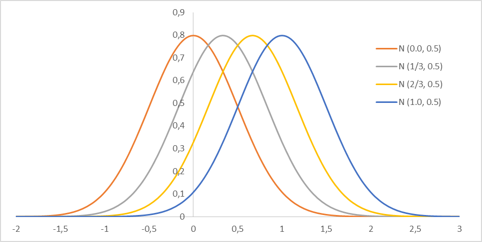
Each distribution in Figure 1 guides the random number generation process of each alternative.
Note that, in spite of the arbitrariness of the values of the standard deviation and the range of means, its values were intended to guarantee that all alternatives have a chance (a very small chance for the least preferred ones) of being chosen as the first candidate.
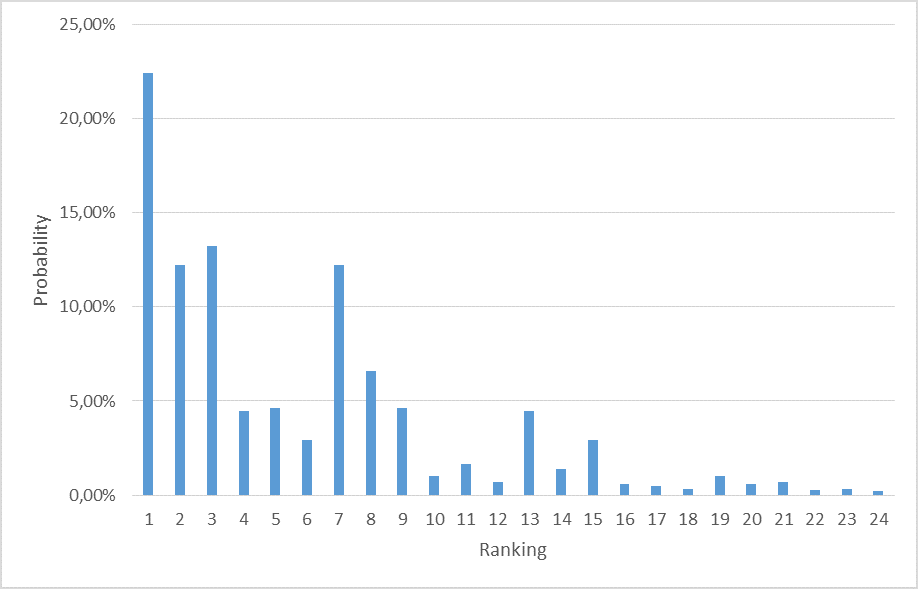
This procedure will generate a set of 24 rankings of 4 alternatives. Table 1 and Figure 2 present the probabilities of each ranking for the distributions in Figure 1 when using the algorithm of random preference generation proposed.
| # | ranking | Prob. (%) | # | ranking | Prob. (%) |
| 1 | a1, a2, a3, a4 | 22.42 | 13 | a3, a1, a2, a4 | 4.44 |
| 2 | a1, a2, a4, a3 | 12.25 | 14 | a3, a1, a4, a2 | 1.41 |
| 3 | a1, a3, a2, a4 | 13.24 | 15 | a3, a2, a1, a4 | 2.91 |
| 4 | a1, a3, a4, a2 | 4.44 | 16 | a3, a2, a4, a1 | 0.60 |
| 5 | a1, a4, a2, a3 | 4.64 | 17 | a3, a4, a1, a2 | 0.46 |
| 6 | a1, a4, a3, a2 | 2.92 | 18 | a3, a4, a2, a1 | 0.31 |
| 7 | a2, a1, a3, a4 | 12.25 | 19 | a4, a1, a2, a3 | 1.00 |
| 8 | a2, a1, a4, a3 | 6.59 | 20 | a4, a1, a3, a2 | 0.60 |
| 9 | a2, a3, a1, a4 | 4.64 | 21 | a4, a2, a1, a3 | 0.70 |
| 10 | a2, a3, a4, a1 | 1.00 | 22 | a4, a2, a3, a1 | 0.28 |
| 11 | a2, a4, a1, a3 | 1.67 | 23 | a4, a3, a1, a2 | 0.32 |
| 12 | a2, a4, a3, a1 | 0.70 | 24 | a4, a3, a2, a1 | 0.21 |
Unit simulation
Each unit simulation is the simulation of both Borda and RSBr for a single scenario. It works as follows:
- Create scenario (n; m);
- For each voter vi, with i ranging from 1 to n:
- Generate Ai (random subset of alternatives of size r);
- Compute the Borda count for the traditional Borda;
- Compute the Borda count for RSBr;
- Calculate the Match Index (MI).
The generation of each random subset Ai have to guarantee that the alternatives will have the same chance of being assigned to any random subset.
Figure 3 shows the results of a unit simulation for a (250; 4) configuration with 2 random alternatives. The distributions of Figure 1 were used for generating the random preferences. For convenience, we have computed the evolution of the Borda count as the voters cast their votes. In practice, it is the equivalent of publishing the partial results of the election after each vote cast.
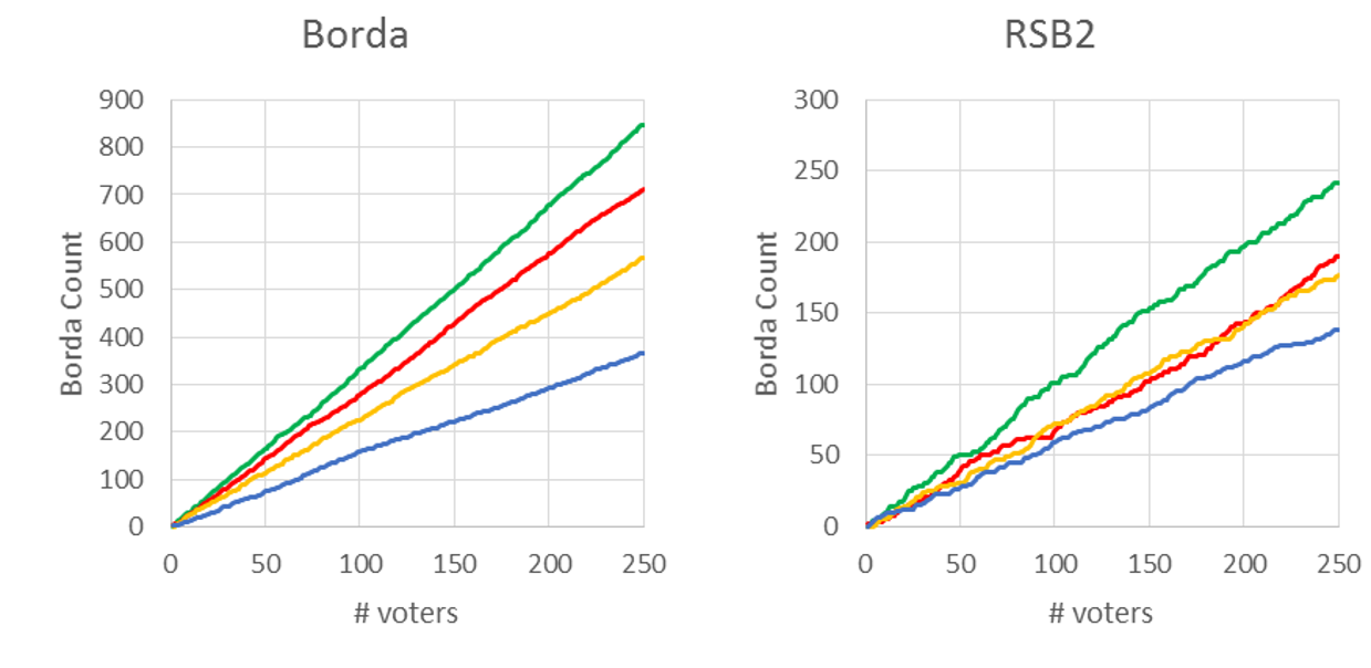
The lines in the graph represents the evolution of the Borda count for all four alternatives in both methods. Note that, as the number of voters increase, the rankings of Borda and RSB2 tend to converge. In this simulation, the Match Index reached its peak (full match) after 221 votes.
In the next subsection, we show the multi-r simulations.
Multi-r simulation
For a given scenario, we define a multi-r simulation as the execution of all possible unit simulations for a single scenario. In other words, for each value of r (ranging from 2 to m), a unit simulation is executed and the match index is calculated.
In Figure 4, we present the results of the multi-r simulation of a (1,000; 10) scenario. The graph indicates how MI evolves as the number of random alternatives increases.
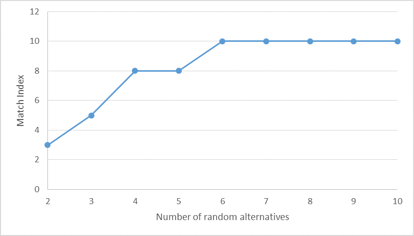
Note that, as the number of random alternatives increase, the match index tends to reach m. It is a rather intuitive result, since the upper bound of the number of random alternatives is in this case 10. In this simulation, the value of MI for r=2 was 3. It means that the comparison of the final rankings of Borda and RSB2 presented only 3 matches. For values of r ranging from 3 to 5, MI was, respectively, 5, 8 and 8. For the remaining values of r (from 6 to 10), MI was equal to 10 (full match).
In the next subsection, we show how we have executed the multi-r simulations for 15 pre-determined configurations.
Multi-configuration simulations
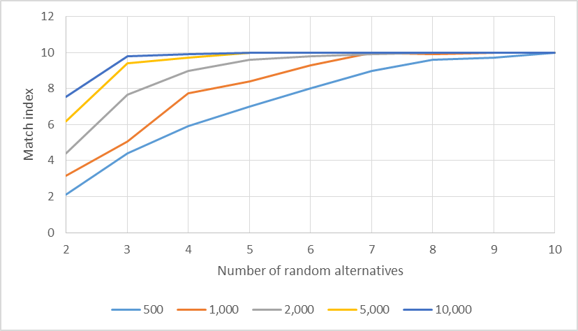
In this subsection, we present the results of the simulations for the configurations in Table 2.
| m | Number of voters | ||||
| 10 | 500 | 1,000 | 2,000 | 5,000 | 10,000 |
| 20 | 2,000 | 5,000 | 10,000 | 20,000 | 40,000 |
| 50 | 5,000 | 10,000 | 40,000 | 70,000 | 100,000 |
For each configuration, we have generated 20 random scenarios and executed a multi-r simulation for each one. We have then calculated the means of MI for each configuration.
Figure 5 presents the results of the simulations for m=10. Each line in the graph represents, for each configuration, the variation of the match index as the number of random alternatives increase. Note that, as expected, r=10 implied MI=10 for all configurations. This is the traditional Borda method. For small values of r, 3 for example, the mean of MI for the configurations (500; 10), (1,000; 10), (2,000; 10), (5,000; 10) and (10,000; 10) was, respectively, 4.4, 5.05, 7.65, 9.4 and 9.8. For r=8, these values reached 9.6, 9.9, 10, 10 and 10. For n equals to 10,000, 5,000, 2,000, 1,000 and 500, the methods converged, i.e. presented the same rankings, respectively, at r equals to 5, 5, 8, 9 and 10.
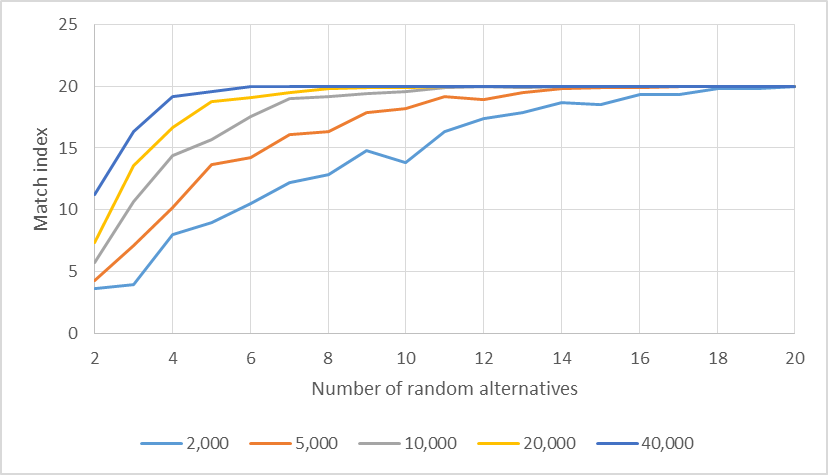
In Figure 6, the lines indicate the evolution of the match index for the configurations in which m=20. One can easily observe that for n=40,000, the match index reaches its peak at r=6 staying unchanged for the remaining values of r. For n equals to 20,000, 10,000, 5,000 and 2,000 the methods converged, i.e. presented the same rankings, respectively, at r equals to 11, 12, 17 and 20.
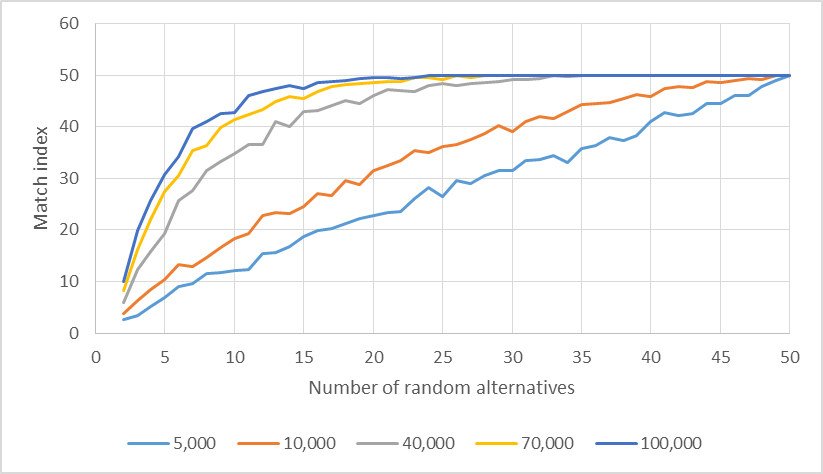
A similar analysis of Figure 7 shows that, for m=50, the methods converge at r equals to 50, 50, 38, 30 and 25 for m equals to 5,000, 10,000, 40,000, 70,000 and 100,000, respectively.
Convergence simulation
The results of the last subsection led us to the following question: For a given number of alternatives, how many voters and random alternatives are necessary to have a full match of Borda and RSBr?
In order to have a first glance of the answer, we have implemented a simulation in which, for a given number of alternatives, we gradually increase the number of voters and check whether the full match is reached. When it is reached, we decrement r and repeat the same process. This cycle repeats until r=2. The algorithm that follows presents the simulation steps:
- Define r = m
- Define n = 100
- Define list = []
- While r ≥ 2:
- Create scenario (n; m)
- Single-run for the scenario with r random alternatives
- Compute MI
- If MI = m:
- r = r-1
- Save tuple (r; n) in list
- Increment n.
In summary, this simulation identifies the population in which the first full match is verified for each value of r.
For each value of m (10, 20 and 50) we have run 20 times the simulation. At the end of the process, we have a list of tuples that indicates the number of voters m in which a full match was verified with r random alternatives.
Figure 8 presents the results of simulations for m=10. For each value of r, the graph depicts the mean of the population in which a full match of Borda and RSBr was first verified.
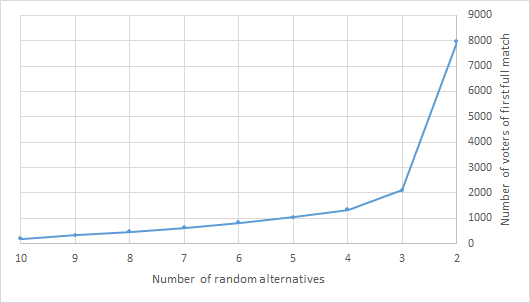
The behavior of the curve indicates that, for values of r ranging from 10 to 3, the corresponding population rose steadily from 200 to 2,000. For r=2, the number of voters increased exponentially and reached 8,000.
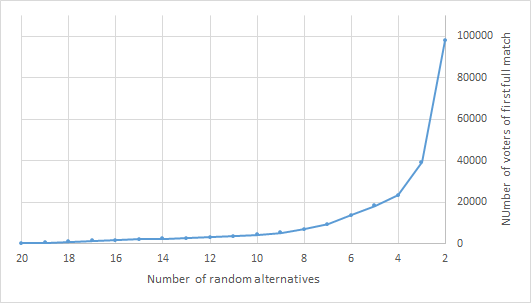
A similar exponential growth is verified in Figure 9 (m=20). For r ranging from 20 to 5, one can identify a gradual increase in the population. Afterwards, the slope of the curve changes and the subsequent values of n grow rapidly.
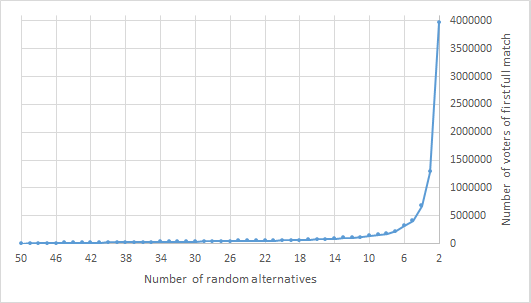
For the simulations with m=50 (Figure 10), the exponential behavior of the curve is even more tangible. After r=10, when the number of voters was around 140,000, the curve begins a clear change in its behavior, leading to approximately 4,000,000 voters when r=2.
In the next sub-section, we present the web experiment implemented to validate RSB.
Web experiment
In order to have a first glance of a real application of the Random-Subset Borda, we have implemented a very straightforward web experiment in which respondents were asked to rank alternatives, juices in this case, according to their preferences. Our goal was to evaluate how the scenario proposed in Figure 3 (m=4, r=2) performed when real people were required to order alternatives in RS Borda and in Borda.
In about 4 months, 365 students and federal employees from the Federal Institute of Education and Technology in Pernambuco and from the Federal University of Pernambuco, both in Brazil, participated in the experiment. The voting system was developed in Python/Django and was made available through the internet.
The entire voting process was divided into four steps:
- present to the voters the goal of the experiment, which was, in summary, to rank juices according to their preferences;
- fill in a form with basic personal information (age and sex);
- rank 2 alternatives;
- rank 4 alternatives.
We have chosen juices of four well known fruits in the region: passion fruit, strawberry, acerola and mangaba (hancornia speciosa).
In the third step, as proposed by RS Borda, we have randomly chosen two alternatives from the set of four juices.
The ranking process was accomplished by a drag and drop tool that allowed the voters to order the alternatives according to their preferences. To minimize any bias in this process, the alternatives were randomly presented to the voters.
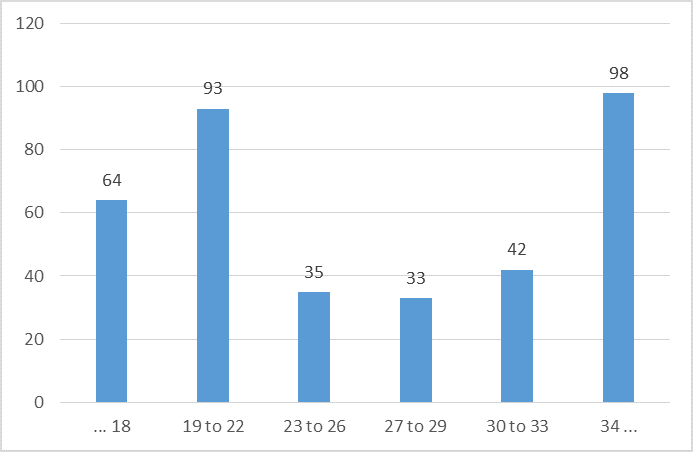
From the set of 365 respondents, we had 160 men and 205 women. Figure 11 presents the distribution of their ages.
The distribution of alternatives in the random subsets are presented in Figure 12.
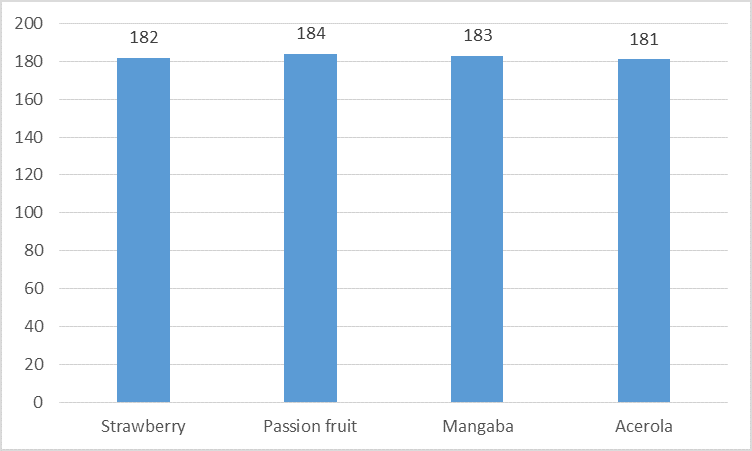
From Figure 12, one can notice that a uniform distribution was used to randomly select the alternatives for the random subsets, i.e., a fair mechanism selected the alternatives and assigned them to the respondents. As expected, in spite of the fairness of the mechanism, small variations in the count of alternatives in the subsets were verified. Passion fruit appeared in 184 subsets, while acerola appeared in 181. Strawberry and mangaba appeared 182 and 183 times, respectively [5].
Figure 13 presents the results of the experiment.
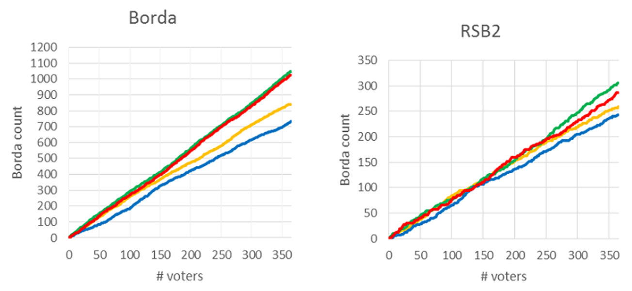
Table 3 presents the final counts for the alternatives in both methods.
| Juice | Borda count | RSB2 count |
| Passion fruit | 1049 | 306 |
| Acerola | 1027 | 287 |
| Strawberry | 842 | 259 |
| Mangaba | 732 | 243 |
Figure 13 showed the evolution of the Borda count for Borda and for RSB2 for the 365 respondents. After 252 voters the methods converged.
Discussion
In this section, we present some discussions about the approaches used to validate RSB.
First, using analytical techniques, we have demonstrated that, for big electorates, RSB and Borda converge to the same outcome. This means that, as the number of voters increase, the results of both methods are the same with probability 1.
In order to have more practical insights regarding the proposed method, we have run several simulations. The results of the simulations indicate some relationships between the number of alternatives (m), the number of voters (n), the number of random alternatives (r) and the match index (MI):
- On keeping m and n fixed, increasing r led to an increase in MI. In spite of the variations identified in the results this trend is verified in all simulations;
- On keeping m and r fixed, increasing n led to an increase in MI;
- For a given m, in order to reach a full match (MI = m), one can either increase n or r;
For fixed values of m and r, the simulations also suggest the existence of thresholds for n. In other words, one can expect that after a certain number of voters the probability of having MI = m tends to 1.
The findings here indicate that, considering the assumptions of transitivity, completeness and IIA, Borda and RSB methods lead to the same results in large electorates. This point was verified in the mathematical model, in all simulations and in the experiment.
It is important to notice that when comparing the simulation presented in Figure 3 (m=4 and r=2) and the results of the web experiment (Figure 13), a relatively small difference in the convergence threshold was verified. While in the simulation the threshold was 221 voters, in the experiment, it was 252. More experiments should be undertaken in future researches in order to verify how the implemented simulation behave in real scenarios.
Conclusion
In this paper, we have proposed the Random-Subset Voting procedure, a new way of combining probability and voting. With this method, a voter will not rank the entire set of alternatives, but a subset of it. This subset is selected by a fair random mechanism that guarantees that all candidates will have the same chance of being assigned to each voter.
We have applied the RSV idea in the context of Borda through the Random-Subset Borda and used three different approaches in the validation of the proposed method: a mathematical analysis of the convergence, a simulation and an experiment. The results of all approaches showed that when the number of voters is large enough RSB and Borda converge to the same outcome.
The results also suggest the existence of thresholds of convergence. We have used the simulations to estimate the number of voters in which a full match between Borda and RSB might occur for different scenarios.
The main goal of this proposal concerns the minimization of the overwhelming effect some voters could face when dealing with many alternatives. In a hypothetical large-scale scenario, we could implement the following experiment. Citizens in a city or a state have to evaluate (rank) 50 projects. After eliciting their preferences and aggregating the results, the top 5 projects will be implemented. Now, assume that instead of analyzing 50 projects, each citizen will be asked to evaluate only 2, chosen randomly. From a theoretical point of view, when the premises already mentioned hold, the results of RSB will match the results of Borda. It means that the voters do not need to evaluate all the projects in order to reach the same collective decision.
This example guides us to another important aspect of RSV: the possibility of bringing into large-scale decisions voting methods like Borda, Condorcet, ranked ballots, etc. These procedures, due to the considerable amount of information required to the voter, could not be used in several contexts. When deciding over 20 or more alternatives for example, some methods are, in practice, unsuitable. With RSV, they could represent feasible alternatives.
Another facet of RSV concerns the premise that humans are not always as rational as some models preconize and that completeness, transitivity and IIA are not verified. In the mathematical modeling and in the simulations, we have shown that RSB and Borda converge when these premises are considered. In real situations, however, one can anticipate that the rational assumptions do not necessarily hold and that the individual rankings of RSB will not be consistent with the rankings of Borda. It is expected that some voters change the relative position of some alternatives when evaluating fewer options. A voter could have a different opinion about some alternatives when evaluating small subsets. One could argue that these changes caused by this “non-rational” behavior would lead to better collective results, since dealing with fewer options will minimize the overwhelming effect that plays a role in such scenarios. However, further investigation of this point needs to be addressed in the future.
An additional concern regarding RSV is the applicability of the procedure in real scenarios. Some might argue that this work can only be taken from a theoretical point of view, but do not have practical implications. Even though we defend that much work has to be accomplished before bringing RSV into our political life, we do believe it could be a real-world tool for decision making, especially if, or when, we move from our traditional indirect democracy to a more direct and online-based one (Santos 1998; Sintomer 2010; Pateman 2012). The applied web experiment was a simple but relevant argument in favor of this idea.
It is important to emphasize that RSV is a concept that could be better applied to situations in which many alternatives are in the choice set. It is not yet clear, however, how many alternatives characterize “many”. Is it 10? 20? In fact, we believe that, depending on the nature of the alternatives and on the number of voters, reducing a set of 6 or 7 alternatives to a random subset of 2 might be appropriate. In other contexts, reducing sets of 20 or 30 to random subsets of 4 or 5 could lead to good social results. In future researches, this issue will be further investigated.
An additional point that must be brought into light is that one can defend the argument that some voters would not agree with the subset assigned to them and state they have been harmed by receiving “poor alternatives”.
Even though we could not yet identify to what extent this argument is valid, we argue that this argument can be considered when representatives are the alternatives. When people choose people, poor candidates might be assigned to many voters and lead to an increase in the abstention levels. However, there are evidences that the increase in the abstention levels can be identified in situations where the number of alternatives is big enough (Cunow 2013). This reasoning needs to be addressed in future researches.
In spite of this consideration, the “very poor alternatives” issue do not play a big role when taking projects or actions. In this situation, the goal of the voters will be to evaluate the alternatives assigned to them and declare their preferences. All the alternatives might be good enough, and the goal would be to define the subset of actions that will be implemented when a specific budget is made available, for example.
One last aspect that needs to be taken into account is the operationalization of the proposal. In fact, if this method was proposed a few decades ago, the applicability of it would have been challenged. Nowadays, however, our technology and ability to deliver private, secure and fast information suggest that dealing with the operational overhead of such a solution would not be a barrier.
Other future researches might include modeling, simulating and implementing experiments of other voting schemes and evaluating how they behave in the context of RSV.
Notes
- There is some confusion in the literature concerning the different definitions of IIA; see Arrow (1950), Ray (1973), Bordes & Tideman (1991) and McLean (1995). In general, these definitions split into two categories: social and individual. The social one, defined by Arrow (1950), concerns changes in relative positions of alternatives in the aggregated ordering when adding alternatives to or removing alternatives from the choice set. The individual one, proposed by Radner & Marschak (1954), and also presented by Sen (1971), under the alpha property definition, considers whether adding to or removing an alternative from the choice set will have impact on the preferences of a voter over the alternatives already in the choice set. It is also studied under the framework of psychology and consumer research as decoy or context effects (Trueblood et al., 2013). In this paper, we adopt the IIA definition from the individual perspective.
- Even though it might seem odd for many, lots have been used many times in our democratic history. In Athens, Venice and Florence, for example, many representatives were chosen by lot. Some scholars even argue that sortition was a core principle of the ancient Athenian democracy and played a crucial role at the time (Headlam 1891; Tridimas 2012; Bouricius 2013, Lockard 2004).
- Nurmi (1983) presents a detailed analysis regarding the difficulty and easiness of voting schemes.
- www.openabm.org/model/4758/.
- A more strict version of the fair mechanism could consider forcing the same count of alternatives in the random subsets. In this case, some voters might get random subsets with r + 1 or r - 1 random alternatives.
References
ADAMS, J. (1997). Condorcet efficiency and the behavioral model of the vote. The Journal of Politics, 59 (4), 1252-1263. [doi:10.2307/2998600]
ALLAIS, M. (1953). Le comportement de l'homme rationnel devant le risque: Critique des postulats et axiomes de l'Ecole Americaine. Econometrica, 21 (4), 503-546.
ANAND, P. (1993). The philosophy of intransitive preference. The Economic Journal, 103 (417), 337-346. [doi:10.2307/2234772]
ARROW, K. J. (1950). A difficulty in the concept of social welfare. The Journal of Political Economy, 58 (4), 328-346.
ARROW, K. J. (1963). Social Choice and Individual Values. New York: John Wiley & Sons.
BARBERÁ, S. (1979). Majority and positional voting in a probabilistic framework. The Review of Economic Studies, 46 (2), 379-389.
BARBERÁ, S. and Pattanaik, P. (1986). Falmagne and the rationalizability of stochastic choices in terms of random orderings. Econometrica, 54 (3), 707-715. [doi:10.2307/1911317]
BISSEY, M., Carini, G. and Ortona, G. (2004). ALEX3 : A simulation program to compare electoral systems. Journal of Artificial Societies and Social Simulation, 7 (3).
BORDES, G., Tideman N. (1991). Independence of irrelevant alternatives in the theory of voting. Theory and Decision, 30, 163-186. [doi:10.1007/BF00134122]
BORDLEY, R. F. (1983). A Pragmatic method for evaluating election schemes through simulation. The American Political Science Review, 77 (1), 123-141.
BOURICIUS, T. (2013). Democracy through multi-body sortition: Athenian lessons for the modern day. Journal of Public Deliberation, 9 (1), 1-19.
CAMERER, C. (1998). Bounded rationality in individual decision making. Experimental Economics, 1 (2), 163-183.
CHAMBERLIN, J. and Cohen, M. (1978). Toward applicable social choice theory : A comparison of social choice functions under spatial model assumptions. The American Political Science Review, 72 (4), 1341-1356. [doi:10.2307/1954543]
CHAMBERLIN, J. (1986). Discovering manipulated social choices: The coincidence of cycles and manipulated outcomes. Public Choice, 51, 295-313.
CHAMBERLIN, J. and Featherston, F. (1986). Selecting a voting system. The Journal of Politics, 48 (2), 347-369. [doi:10.2307/2131097]
CHENG, S. Long, J. (2007). Testing for IIA in the multinomial logit model. Sociological Methods & Research, 35 (4), 583-600.
COUGHLIN, P. and Nitzan, S. (1981). Electoral outcomes with probabilistic voting and Nash social welfare maxima. Journal of Public Economics, 15 (1), 113-121. [doi:10.1016/0047-2727(81)90056-6]
CUNOW, S. (2013). Too Much Choice? Abstention Rates, Representation and the Number of Candidates. Working paper, University of California.
DANAN, E. and Ziegelmeyer, A. (2006). Are Preferences Complete? An Experimental Measurement of Indecisiveness Under Risk. Working Paper, Max Planck Institute of Economics.
EHLERS, L., Peters, H. and Storcken, T. (2002). Strategy-proof probabilistic decision schemes for one-dimensional single-peaked preferences. Journal of Economic Theory, 105(2), 408-434.
FISHBURN, P. (1975). A probabilistic model of social choice: A comment. The Review of Economic Studies, 42 (2), 297-301. [doi:10.2307/2296538]
FISHBURN, P. (1991). Nontransitive preferences in decision theory. Journal of Risk and Uncertainty, 4 (2), 113-134.
FISHBURN, P. and Gehrlein, W. (1977). Towards a theory of elections with probabilistic preferences. Econometrica, 45 (8), 1907-1924. [doi:10.2307/1914118]
FRY, T.R., HARRIS, M. N. (1996). A Monte Carlo study of tests for the independence of irrelevant alternatives property. Transportation Research Part B: Methodological, 30(1), 19-30.
GEHRLEIN, W. (2004). Consistency in measures of social homogeneity: A connection with proximity to single peaked preferences. Quality and Quantity, 38 (2), 147-171. [doi:10.1023/B:QUQU.0000019391.85976.65]
GEHRLEIN, W. (2006). Condorcet's Paradox. Berlin: Springer Verlag.
GEHRLEIN, W. and Lepelley, D. (2000). The probability that all weighted scoring rules elect the same winner. Economics Letters, 66 (2), 191-197. [doi:10.1016/S0165-1765(99)00224-4]
GEHRLEIN, W. and Fishburn, P. (1978). Probabilities of election outcomes for large electorates. Journal of Economic Theory, 19 (1), 38-49.
GEHRLEIN, W. and Fishburn, P. (1981). Constant scoring rules for choosing one among many alternatives. Quality and Quantity, 15 (2), 203-210. [doi:10.1007/BF00144260]
GIBBARD, A. (1977). Manipulations of schemes that mix voting with chance. Econometrica, 45 (3), 665-681.
HEADLAM, J. (1891). Election by Lot at Athens. Cambridge: Cambridge University Press.
INTRILIGATOR, M. (1973). A probabilistic model of social choice. Review of Economic Studies, 40 (4), 553-560.
INTRILIGATOR, M. (1982). Probabilistic models of social choice. Mathematical Social Sciences, 2, 157-166. [doi:10.1016/0165-4896(82)90064-6]
IYENGAR, S. and Lepper, M. (2000). When choice is demotivating: Can one desire too much of a good thing?. Journal of Personality and Social Psychology, 79 (6), 995-1006.
JOHNSON, P. (1999). Simulation modeling in political science. American Behavioral Scientist, 42 (10), 1509-1530. [doi:10.1177/0002764299042010004]
JONES, B., Radclif, B., Taber, C., Timpone, R. (1995). Condorcet winners and the paradox of voting: probability calculations for weak preference orders. The American Political Science Review, 89 (1), 137-144.
KEMENY, J. (1959). Mathematics without numbers. Daedalus, 88(4), 577-591.
KOLLMAN, K., Miller, J., Page, S. (2012). Adaptive parties in spatial elections. Political Science, 86 (4), 929-937.
KOLMOGOROV, A. N. (1956). Foundations of the Theory of Probability. Chelsea, New York, 1933. Trans. N. Morrison.
LOCKARD A. (2004). Sortition. In D. Rowley and F. Schneider (Eds.), In The Encyclopedia of Public Choice (pp. 857-860). Springer US.
LUDWIN, W. (1976). Voting methods: A simulation. Public Choice, 25 (1), 19-30. [doi:10.1007/BF01726328]
MCFADDEN, D., Train, K. and Tye, W. (1977). An application of diagnostics tests for the independence from irrelevant alternatives property of the multinomial logit model. Transportation Research Record, 637, 39-46.
MCKELVEY, R. and Patty, J. (2006). A theory of voting in large elections. Games and Economic Behavior, 57 (1), 155-180. [doi:10.1016/j.geb.2006.05.003]
MCLEAN, I. (1995). Independence of irrelevant alternatives before Arrow. Mathematical Social Sciences, 30 (2), 107-126.
MERRILL III, S. (1984). A Comparison of efficiency of multicandidate electoral systems. American Journal of Political Science, 28 (1), 23-48. [doi:10.2307/2110786]
NAU, R. (2006). The shape of incomplete preferences. Annals of Statistics, 34 (5), 2430-2448.
NITZAN, S. (1975). Social preference ordering in a probabilistic voting model. Public Choice, 24(1), 93-100. [doi:10.1007/BF01718418]
NURMI, H. (1983). Voting procedures: a summary analysis. British Journal of Political Science, 13(2), 181-208.
NURMI, H. (2002). Voting Procedures under Uncertainty. Berlin: Springer. [doi:10.1007/978-3-540-24830-9]
NURMI, H. (2014). Are we done with preference rankings? If we are, then what?. Operations Research and Decisions, 24 (4), 63-74.
PATEMAN, C. (2012). Participatory democracy revisited. Perspectives on politics, 10(1), 7-19. [doi:10.1017/S1537592711004877]
RADNER, R., MARSCHAK, J. (1954). Note on some proposed decision criteria. Decision Process, 61-68.
RAY, P. (1973). Independence of irrelevant alternatives. Econometrica: Journal of the Econometric Society, 41(5), 987-991. [doi:10.2307/1913820]
DE SOUSA SANTOS, B. (1998). Participatory budgeting in Porto Alegre: toward a redistributive democracy. Politics & Society, 26(4), 461-510.
SCHEIBEHENNE, B., Greifeneder, R. and Todd, P. M. (2010). Can there ever be too many options? A meta-analytic review of choice overload. Journal of Consumer Research, 37 (3), 409-425. [doi:10.1086/651235]
SCHUMACHER, G. and Vis, B. (2012). Why do social democrats retrench the welfare state? A simulation. Journal of Artificial Societies and Social Simulation, 15(3), 4: https://www.jasss.org/15/3/4.html. [doi:10.18564/jasss.1959]
SCHWARTZ, B. (2004). The paradox of choice. New York: Harper-Collins.
SCHWARTZ, B., Ward, A., Monterosso, J., Lyubomirsky, S., White, K. and Lehman, D. R. (2002). Maximizing versus satisficing: happiness is a matter of choice. Journal of Personality and Social Psychology, 83(5), 1178-1197.
SEN, A. (1971). Choice functions and revealed preference. The Review of Economic Studies, 38 (3), 307-317. [doi:10.2307/2296384]
SIMON, H. A. (1955). A behavioral model of rational choice. The Quarterly Journal of Economics, 69(1), 99-118.
SINTOMER, Y. (2010). Random selection, republican self-government, and deliberative democracy. Constellations, 17 (3), 472-487. [doi:10.1111/j.1467-8675.2010.00607.x]
TIDEMAN, T. N., & Plassmann, F. (2012). Modeling the outcomes of vote-casting in actual elections. In Electoral Systems (pp. 217-251). Springer Berlin Heidelberg.
TRIDIMAS, G. (2012). Constitutional choice in ancient Athens: The rationality of selection to office by lot. Constitutional Political Economy, 23 (1), 1-21. [doi:10.1007/s10602-011-9112-1]
TRUEBLOOD, J. S., Brown, S. D., Heathcoat, A. and Busemeyer, J. (2013). Not just for consumers: Context effects are fundamental to decision making. Psychological Science, 24 (6), 901-908.
WALPOLE, R. E., Myers R. H., Myers S. L., Ye, K. (2012). Probability and Statistics for Engineers and Scientists. Boston: Prentice Hall.
ZECKHAUSER, R. (1969). Majority rule with lotteries on alternatives. The Quarterly Journal of Economics, 83 (4), 696-703.