
Introduction
A demographically viable population can be defined as one that persists for a certain length of time despite stochastic perturbations in mortality, fertility, and sex ratio. Small populations are potentially susceptible to extinction through these stochasticities: the smaller the population, the greater the proportion of the population is represented by each individual, and the greater impact of each birth and death on the characteristics of the entire population (Moore 2001, p. 403; Shaffer 1981; Wobst 1975). The link between viability and size is a central principle of population biology. The minimum viable population (MVP) size is the population size above which stochastic factors do not pose a significant threat to the survival of the population over some defined length of time (Shaffer 1981). MVP size is typically assessed over a span of time many generations in duration in order to allow the effects of stochastic perturbations to play out.
In all species, reproductive variables such as fecundity, reproductive strategy, and maturation rates have significant impacts on the size of population that is "viable" under different circumstances (see Sakai et al. 2001; Shaffer 1981; White et al. 2008). In human populations, the cultural rules affecting marriage also potentially impact viability by defining or restricting a person’s pool of potential mates. A wide range of marriage behaviors has been observed among ethnographic hunter-gatherers (e.g., see Binford 2001; Kelly 1995; Murdock 1967). Clarifying how differences in fertility and marriage affect the demographic viability of small populations is relevant to understanding the size and structure of both ethnographic hunter-gatherer societies and those that we are attempting to understand archaeologically. Finding the lower size limits of demographically viable human populations is of particular interest to anthropologists studying how human societies adapt to different environments and colonize empty landscapes.
I use an agent-based model (ABM) to systematically explore how variability in marriage behaviors and mortality conditions affects the ability of hunter-gatherer populations of varying size to sustain themselves over long periods of time when growth is constrained. An ABM allows us represent the human behaviors that we can document ethnographically (such as birth, marriage, reproduction, and death) as operational "rules" for human-level behavior, create a system of actors who interact according to these rules, set the system in motion, and characterize the outcomes in terms of aggregate patterns. In contrast to equation-based demographic models, this type of model permits stochasticity in mortality, fertility, and sex ratio to operate at the correct "human" level and ultimately affect survival at the population level. Through systematic experimentation, cause-effect relationships between these two levels can be investigated as an empirical problem, allowing us to use modeling as tool for building theory about the minimum size of demographically viable hunter-gatherer populations.
In this paper, a "viable" population is defined as one that survives over a span of 400 years. Under the conditions investigated here, experiment results show that model populations greater than 150 persons are largely unthreatened by the normal stochastic perturbations in mortality, fertility, and sex ratio that may cause smaller populations to go extinct. MVP size is smaller when marriage rules are less restrictive, as fewer constraints on marriage allow a population to capitalize on a greater proportion of the finite female reproductive span. While some aspects of my results are in accord with those of previous modeling work (i.e., Moore 2001; Wobst 1974), they provide no support to the assertion that a human population size on the order of 500 or so is necessary to ensure demographic viability.
Background
The nature of mobile hunting-gathering adaptations produces a tension between the economics of subsistence and the necessities of demography. Many ethnographically-documented hunter-gatherer populations spend at least part of the year in dispersed, autonomous foraging groups generally containing less than 35 persons (Binford 2001; Kelly 1995). The size and mobility behaviors of these foraging groups are strongly conditioned by subsistence ecology, which often makes it impossible to support larger aggregations of persons for extended periods of time (Binford 1980, 1983, 2001; Kelly 1995). While these small foraging groups constitute functional economic units for subsistence purposes, they are not presumed to be demographically self-sustaining over the course of many generations. Thus groups large enough to be demographically viable are too large to be economically viable, while groups small enough to be economically viable on a day-to-day basis are not demographically viable over the long term. Ethnographic hunter-gatherer systems "solve" this dilemma by using cultural mechanisms (e.g., kinship, exchange, and personal/group mobility) to build and maintain a social system that binds together a dispersed population, facilitating the transfer of information and persons between groups (see White 2012).
Study of relationships between marriage behaviors, population size, and demographic viability in hunter-gatherer social systems has been pursued by both ethnographic research and model-based analysis. Ethnographic research has been used to identify patterns in the sizes of hunter-gatherer systems (e.g., Birdsell 1953, 1958, 1968; Hamilton et al. 2007), document behaviors affecting marriage and reproduction (e.g., Binford 2001; Kelly 1995), and collect demographic data that can be used to characterize living populations (e.g., Hewlett 1991; Hill et al. 2007; Pennington 2001). Model-based analysis has been used to estimate the minimum sizes of hunter-gatherer mating networks (Wobst 1974), explore the relationships between marriage behaviors and fertility (Wobst 1975), and evaluate demographic aspects of colonization models (Moore 2001).
The influential studies of Birdsell (1953, 1958, 1968) and Wobst (1971, Wobst 1974) presumed that the population size of hunter-gatherer social systems would be conditioned by: (1) limitations on the minimum size required for a population to be demographically viable; and (2) the "cost" of maintaining communication across a system of dispersed groups under conditions of very low population density. In combination, these forces would produce social systems of some "equilibrium" size: large enough to be demographically viable but not so large as to be too expensive to maintain. They reasoned that the size of hunter-gatherer social systems should therefore be close to the minimum size necessary to encompass a demographically viable population (Wobst 1974, pp. 154-155).
Birdsell (1953, 1958, 1968) approached the problem of determining equilibrium size by considering ethnographic data from Australia. He noted that the size of "dialectical tribes" of Australian hunter-gatherers had a central tendency of around 500 persons, and reasoned that endogamous social systems of this size were probably also typical of Paleolithic hunter-gatherers. It is worth pointing out, as Birdsell (1953, p. 197) himself did, that the number 500 was a statistical abstraction produced from disparate sources of ethnographic data: the documented size range of Australian "tribes," while varying around a central tendency of about 500 persons, commonly included groups of less than 200 (see Birdsell 1953, Figure 8, 1958, p. 186; Kelly 1995, pp. 209-210).
Wobst (1971, 1974) used a computer simulation to explore the sizes of hunter-gatherer populations necessary to ensure the availability of mating partners over the long term. Following Yellen and Harpending (1972), he defined the minimum equilibrium size (MES) of a population as "the mean and median number of persons that live in the intervening distance between 2 marriage partners" (Wobst 1974, 157). In his simulation, a population divided into groups of 25 people was arrayed in a grid of hexagonal cells. When a male in the population reached marriageable age (15 years old), he systematically searched for a mate in the surrounding population, beginning with the spatially nearest groups. Results from model runs (n = 40) lasting 400 years returned MES values between 79 and 332 people (Wobst 1974, pp.162-163). Systems in this size range would have occupied 1 or 2 tiers of hexagonal grid cells each containing 25 people, leading Wobst to estimate that, in populations that are spatially structured like those in his model, 175 to 475 people would constitute the mean size of a maximum band where the availability of mating partners could be guaranteed. Wobst’s MES estimate of 475 people resonated with the conclusions of Birdsell’s work, reinforcing the earlier characterization (see Lee and DeVore 1968, pp. 245-248) of 500 as a "magic number" in hunter-gatherer demography.
Moore (2001) used a simulation model to explore the extinction of small human populations in several colonization scenarios. Like Wobst’s (1974) model, Moore’s model represented mortality, fertility, and marriage at the level of the individual and contained provisions for adjusting marriage rules. Starting populations of varying size were "set ashore" and allowed to persist until they went extinct or began growing rapidly (depending on conditions). At low fertility rates, populations varying in initial size from 4 to 60 persons invariably went extinct. There was a general positive relationship between the starting size of the population and the mean number of years before the population went extinct. At high fertility rates, very small (ten person) groups that survived the initial "stochastic crisis" often went on to experience rapid growth in population. Moore (2001) offered no formal definition of viability to frame his results, but concluded that
"no population size at low fertility and/or high mortality is sufficiently large to guarantee the success of a colonizing group. But on the other hand, every population, no matter how disadvantageous its demographic conditions might be, has some chance of survival, even for hundreds or thousands of years" (Moore 2001, p. 405).
This statement encapsulates the challenges of understanding demographic viability among the small (and sometimes potentially very small) populations we encounter when considering so many aspects of past hunter-gatherer systems. Of all the analyses performed to try to elucidate aspects of prehistoric hunter-gatherer demography, studies that have attempted to realistically grapple with the impacts of stochasticity in small populations are in a distinct minority. Equation-based models that assume infinite populations, fixed birth/death rates, and/or random mating are of limited utility for exploring demography in small populations where individual-level stochastic variation is an important factor (cf. Wobst 1975, p. 76). The studies of Birdsell and Wobst have enjoyed considerable influence over the last forty years, perhaps in part because they have existed in a near-vacuum of subsequent theory-building work. The "magic number 500" retains currency as a simple explanation for why hunter-gatherer social systems appear to occur in a limited range of sizes relative to those of other human societies, and Wobst’s (1974) study is often the sole paper cited in support of the general idea that hunter-gatherer populations must be of some minimum size that is larger than that of the foraging group in order to be "viable" or "effective" or "self-sustaining."
The model that I utilize in this paper has many parallels with the models of Wobst (1974) and Moore (2001). Like those models, it represents each person as an individual entity, allowing heterogeneity within the population and permitting stochasticity to operate at the correct level. Perhaps the most important difference between this model and those of Wobst (1974) and Moore (2001) is that the model used here incorporates household-level feedback mechanisms that affect decisions about marriage, reproduction, and infant mortality. This is important because of the place of the family/household as a fundamental economic and social unit in hunter-gatherer systems (e.g., Binford 2001, p. 309; Helm 1965, p. 379; Jarvenpa and Brumbach 1988, p. 607; Keen 2004; Wobst 1971, p. 62). Incorporating representations of basic household productive/reproductive behaviors and constraints allows us to let stochastic effects play out in model systems that more closely resemble those we are trying to understand.
Model Description
The model used for this analysis is version 3 of the ForagerNet3_Demography model (hereafter FN3D_V3). The model was written in the Java programming language and built initially using Repast J. The data used here were produced after the model was converted to run in Repast Simphony. Documentation of Repast can be found at www.repast.sourceforge.net. Raw code and description for the FN3D_V3 model are available online at www.openabm.org (White 2016b). This section provides a general overview of the design, operation, and methods of the model and describes in detail the representation of marriage restrictions that are specific to the analysis in this paper.
General design and operation
The model has three main "levels:" person, household, and the system. Each agent in the model represents an individual person that is a discrete entity with a unique identity. Households are co-residential groupings of persons that form through marriage and change in size and composition primarily through marriage, reproduction, and mortality. Occasionally households can include members that are not related by biological descent, marriage, or marriage to a common partner (e.g., when both parents in a household die and their "orphan" children become part of a different household). The dependency ratio of a household (the ratio of the number of consumers to the number of producers) is a key factor in probability-based, household-level decisions about reproduction, marriage, and infanticide (see below). For the experiments discussed here, persons are counted as producers at age 14. A dependency ratio of 1.75, considered "typical" of hunter-gatherers (Binford 2001, p. 230), was used to perform economic calculations. The system of the model is composed of all persons and households in existence at a given point in time.
Social links classify relationships between pairs of living persons and are used to define which pairs of persons are prohibited from marrying. Family links indicate a consanguineal (i.e., blood descent) relationship. Kinship and marriage links are links of affinity (i.e., created through marriage). Co-resident links are established between individuals that co-reside in a household but do not qualify for family, marriage, or kin status. A change in the nature of the relationship between two persons will trigger a change in the class of the social link that connects the two persons.
Model-level parameters set conditions for all persons or all households in the world and define aspects of the system: all persons become eligible to marry at the same age, for example. The model was intentionally configured to remove the spatial components of interaction and behavior. This eliminates the potential effects of information flow, mobility, and population density on the analysis performed here.
At the startup of each run, the model produces an initial population of a specified number of persons of random sex and random age between 15 (the age at which the potential for reproduction and pair-bonding begins) and 20. The initial households in a model run are created through random marriages between eligible males and females in the initial population.
Time passes in the model in the form of discrete steps, each representing one week (5200 steps representing 100 years). Following the creation of initial persons and households, the model takes a step and initiates a sequence of operations that includes the methods for pair-bonding, reproduction, and death (see White 2016b). This same sequence of operations is repeated in every subsequent step until the model has completed a specified number of steps. Data required for computing relevant variables (mean population size, total fertility rate, mean female age at marriage, mean percentage of polygynous marriage, etc.) are collected during the second half of a run. Summary data are calculated at the end of a run and appended to a data file for analysis.
Methods
The main methods of interest in this use of the FN3D_V3 model are the marriage, reproduction, and mortality methods.
Marriage. Each male at or above the age of 15 (ageOfMaturity) will enter the marriage methods at each step. A potential female mate is randomly chosen from the pool of unmarried females of reproductive age. The model then checks to confirm that the pairing would not violate the set marriage restrictions (see below) nor create an economically unviable household (e.g., if the female has many dependents from a previous bonding where the male has died). If these conditions are met, the male and female each perform a sequence of economic calculations that computes the probability that they will marry (see White 2013, pp. 132-135, 2016b). If the male is already married and polygyny is permitted, the male calculation is based on the economic utility of adding an additional female to his existing household. The female calculation is based on a comparison between the dependency ratio in her current household (typically with her birth family) and the dependency ratio of the household she would join (e.g., as an additional female mate) or form with the male. All single males of suitable age will attempt to marry each step with 100 percent probability.
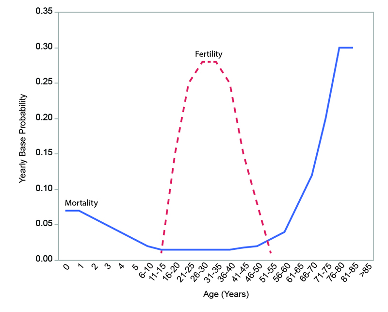
Reproduction. Although the biological potential for female reproduction in the model extends from ages 11 through 55, only currently married females that are not in a period of post-partum amenorrhea are eligible to become pregnant. The base probability of a female becoming pregnant during a given step is calculated by using an age-specific fertility schedule (Figure 1; White 2016b) similar to that documented for the !Kung (Howell 1979) and the Ache (Hill and Hurtado 1996). The peak reproductive years are between ages 21 and 40.
The dependency ratio of a household is the ratio of consumers (the total number of persons in a household) to producers (the number of persons who are actively procuring and/or preparing food). In the model, the dependency ratio of a household affects the reproductive behavior of the household. The probability of pregnancy is reduced if the addition of another child would raise the household’s dependency ratio above 1.75 (1.75 was chosen to represent the dependency ratio of a "typical" hunter-gatherer household based on ethnographic data presented by Binford 2001, p. 230). This represents the existence of mechanisms for avoiding pregnancy based on household-level economics. The chance of avoiding pregnancy is determined by first calculating how much above 1.75 the dependency ratio would rise if another child were to be added and then taking this amount as a percentage of 1.75 (e.g., the chance of avoidance is 100 percent if another child would raise the dependency ratio of the household to 3.5). Successful reproduction results in the creation of a child of random sex who is then added to the household.
The reproduction methods also include a mechanism for terminating the life of a newborn infant (i.e., committing infanticide). The chance of infanticide is calculated using the dependency ratio in the same way as avoidance of procreation: the difference is that the birth and subsequent death of a child figure into infant mortality rates where avoidance of procreation does not. The sex of a child does not affect the probability of infanticide in the model.
Mortality. Each person is exposed to a risk of death at each step. The yearly base probabilities of death are age-specific and follow a pattern similar to that documented for the Ache (Hill and Hurtado 1996) and the Tsimane (Gurven and Kaplan 2007) (see Figure 1). If a person reaches a certain maximum age (set by the value of the parameter maxAge), death is automatic. Infant mortality is increased from the base probabilities in the model through the economically-sensitive infanticide mechanism.
The model uses a global feedback mechanism between mortality rates and population size to stabilize the size of the population (see White 2016a, 2016b). A model-level parameter (popMortAdjustPoint) specifies the population size above which all probabilities of death are increased and below which all probabilities of death are decreased. At each step, the model calculates the variable popMortAdjustment by comparing the current size of the population to the size of the population specified by popMortAdjustPoint. If the current population is 605, for example, and popMortAdjustPoint = 500, the popMortAdjustment is 1.21 (605/500). If the current population is 400 and popMortAdjustPoint = 500, the popMortAdjustment is 0.8 (400/500).
The probability of death for a particular person is calculated by first multiplying that person’s age-specific probability of death per step by the set value of mortalityMultiplier, a model-level parameter that is used to adjust the strength of the feedback between mortality and population size. That probability is then multiplied by the calculated value of popMortAdjustment to arrive at the probability that the person will die that step. In the case of a 25-year-old (with a yearly base probability of death of 0.015) in a population of 605 persons with a popMortAdjustPoint of 500 and a mortalityMultiplier of 1.8, for example, the probability of death each step is 0.000628 ((0.015/52) * (605/500 * 1.8)), 0.0327 each year.
Adjustment of the value of mortalityMultiplier can be used to produce a continuous range of low to high mortality conditions while maintaining the shape of the age-specific curve shown in Figure 1. For the experiments conducted here, settings of 1 (no adjustment), 2 (doubled mortality probabilities), and 4 (quadrupled mortality probabilities) were used to simulate a range of mortality conditions. The value of popMortAdjustPoint was set to the same value as the initial number of persons. Note this does not mean that population size stabilized at that value: it simply means that the base probabilities of death were positively or negatively adjusted based on whether population size is above or below that value. At a given value of popMortAdjustPoint, the particular size at which a model population stabilizes is a product of the balance between fertility and mortality. Populations with more severe mortality conditions stabilize at sizes significantly below popMortAdjustPoint.
Marriage behaviors and constraints
Restrictions on marriage are controlled by a set of three parameters (Table 1, Figure 2).
| Parameter | Function | Settings |
| pairBondMode | Specifies whether or not polygynous marriage is permitted | 1 = monogamous marriage only; 2 = polygynous marriage permitted |
| pairBondRestrictionMode | Specifies the mode of "kin-based" restrictions on marriage | 0 = no restrictions; 1 = "basic" incest taboo; 2 = incest taboo includes all kin; 3 = incest taboo includes marriage divisions |
| numMarriageDivisions | Specifies number of endogamous marriage divisions within population | 1 = no divisions affecting marriage; 2 = population divided into two endogamous groups; 3 = population divided into three endogamous groups; etc. |

The parameter pairBondMode controls whether or not polygynous marriage is permitted. If polygyny is prohibited (pairBondMode = 1), only unmarried males are eligible to marry. If polygyny is permitted (pairBondMode = 2), each male of reproductive age is eligible to marry each step. When polygyny is permitted, person-level decisions about polygynous marriage are affected on a case-by-case basis by the male and female economic calculations discussed above.
The parameter pairBondRestrictionMode specifies the extent of a "kinship-based" incest taboo that prohibits marriage between pairs of persons related by kinship and/or descent. When the value of pairBondRestrictionMode is 0, there is no incest taboo: any eligible female of reproductive age may marry any eligible male of reproductive age. The male designated "ego" in Figure 2a is not prohibited from marrying any of the 11 females in the diagram. Human systems that completely lack cultural rules restricting marriage are unknown ethnographically: pairBondRestrictionMode 0, therefore, can serve as a limiting case representing a minimum restriction of marriage beyond that which has been documented.
When the value of pairBondRestrictionMode is set to 1, the model imposes a "basic" incest taboo: marriage is prohibited between all pairs of individuals connected by family links and any two individuals related as blood aunt/uncle – niece/nephew (Figure 2b). Marriage is also prohibited between any two persons who have previously co-resided in the same household, whether related as family or not. Note that marriage is not prohibited between cousins or between a husband and his wife’s sisters or a wife and her husband’s brothers. This is consistent with the occurrence of these kinds of marriages in many hunter-gatherer societies (e.g., see Kelly 1995; Murdock 1967). In pairBondRestrictionMode 1, the male designated "ego" in Figure 2b would be prohibited from marrying seven of the 11 females in the diagram.
In pairBondRestrictionMode 2, marriage is prohibited between all pairs of individuals connected by kin ties in addition to all pairs of individuals prohibited from marrying in pairBondRestrictionMode 1. This would prevent ego from marrying his female cousin, but not an aunt that is not related through blood descent (Figure 2c).
In pairBondRestrictionMode 3, a set of "marriage divisions" is created to subdivide the population into endogamous groups. The imposition of endogamous marriage divisions in the model represents, in abstract, a cultural system that serves to restrict the pool of potential marriage partners available to each individual in addition to the restrictions imposed by the "basic" incest taboo (as shown in Figure 2b). The section and subsection systems of Australian hunter-gatherer societies are one ethnographic example where non-kinship cultural divisions of the population serve to restrict marriage (see Keesing 1975; Meggitt 1968; Murdock 1965; Yengoyan 1968). The naming system used by the San is another (see Lee 1984, p. 68; Lewis-Williams 1982, p. 436).
The parameter numMarriageDivisions controls the number of marriage divisions which are created. Membership in one of these divisions is determined at birth through the assignment of a random number. When the value of this parameter is set to 4, for example, a random integer between 1 and 4 is generated when a person is born. The person stores this number. When the person is eligible to marry, the pool of potential mates is limited to those with identical numbers. When there are four marriage divisions, approximately three-quarters of the population is considered to be unsuitable for marriage from the perspective of a given individual. In the model, the membership of marriage divisions is independent from kinship and family.
Model Experiments and Results
A set of experiments was performed to evaluate the relationships between population size, cultural restrictions on marriage, and the demographic viability of a population over a fixed span of time. The baseline age-specific mortality probabilities were varied across three sets of runs by adjusting the value of mortalityMultiplier. The goal of these experiments was to explore how cultural restrictions on marriage affected minimum viable population (MVP) size under different mortality conditions. Values for key parameters of the experiments are provided in Table 2.
| Parameter | Description | Value |
| initNumPersons | Number of persons created at start of a model run | 2-500 (variable) |
| popMortAdjustPoint | Population size above which base probabilities of mortality are increased and below which base probabilities of mortality are decreased | 2-500 (set to same value as initNumPersons) |
| popMortAdjustMult | Strength of mortality-based feedback mechanism for stabilizing population size | 1 (constant) |
| ageAtMaturity | Age (in years) at which a person is eligible to marry (and therefore eligible to reproduce) | 15 (constant) |
| agetAtProduction | Age (in years) at which a person is counted as a "producer" for purposes of calculating the dependency ratio of a household | 14 (constant) |
| maxAge | Maximum age (in years) a person may attain | 86 (constant) |
| maxPPA | Maximum duration (in weeks) of post-partum amenorrhea | 72 (constant) |
| ageAtWeaning | Age (in years) at which children are weaned | 3 (constant) |
| sustainableCP | Value of dependency ratio considered "normal;" a dependency ratio > sustainableCP has positive effect on probabilities of avoiding reproduction or committing infanticide | 1.75 (constant) |
| fertilityMultiplier | Adjusts the base age-specific probabilities of pregnancy by a set factor | 1 (constant) |
| mortalityMultiplier | Adjusts the base age-specific probabilities of death by a set factor | 1, 2, or 4 (variable) |
Minimum viable population (MVP) size is defined here as the population size that resulted in survival over a 400 year time span in 95 percent of experiment runs. The 400-year period was chosen to match the length of time used in Wobst’s (1974) landmark simulation study. Assuming generations lasting about 20 years, the 400-year period spans 20 generations.
Basic information about the settings and sample sizes of the MVP experiments is provided in Table 3. Five thousand runs were performed at each combination of settings, randomly varying initial population between 2 and 500 persons. The value of popMortAdjustPoint was set to match the initial population size. Aggregate data on demographic variables (mean fertility and mortality rates, inter-birth interval, male and female ages at marriage, and the percentage and intensity of polygyny) were recorded during the last half of each run and reported on the final step. Five thousand additional runs (one of which was dropped in data transfer) were performed at initial population levels of 501-1000 for one set of conditions (marriage settings 1-3-8; mortalityMultiplier = 4) to determine MVP size.
| mortality Multiplier | pairBondMode | pairBond RestrictionMode | numMarriageDivisions | n runs |
| 1 | 1 (monogamous) | 0 | 1 | 5000 |
| 1 | 1 (monogamous) | 1 | 1 | 5000 |
| 1 | 1 (monogamous) | 2 | 1 | 5000 |
| 1 | 1 (monogamous) | 3 | 2 | 5000 |
| 1 | 1 (monogamous) | 3 | 4 | 5000 |
| 1 | 1 (monogamous) | 3 | 8 | 5000 |
| 1 | 2 (polygynous) | 0 | 1 | 5000 |
| 1 | 2 (polygynous) | 1 | 1 | 5000 |
| 1 | 2 (polygynous) | 2 | 1 | 5000 |
| 1 | 2 (polygynous) | 3 | 2 | 5000 |
| 1 | 2 (polygynous) | 3 | 4 | 5000 |
| 1 | 2 (polygynous) | 3 | 8 | 5000 |
| 2 | 1 (monogamous) | 0 | 1 | 5000 |
| 2 | 1 (monogamous) | 1 | 1 | 5000 |
| 2 | 1 (monogamous) | 2 | 1 | 5000 |
| 2 | 1 (monogamous) | 3 | 2 | 5000 |
| 2 | 1 (monogamous) | 3 | 4 | 5000 |
| 2 | 1 (monogamous) | 3 | 8 | 5000 |
| 2 | 2 (polygynous) | 0 | 1 | 5000 |
| 2 | 2 (polygynous) | 1 | 1 | 5000 |
| 2 | 2 (polygynous) | 2 | 1 | 5000 |
| 2 | 2 (polygynous) | 3 | 2 | 5000 |
| 2 | 2 (polygynous) | 3 | 4 | 5000 |
| 2 | 2 (polygynous) | 3 | 8 | 5000 |
| 4 | 1 (monogamous) | 0 | 1 | 5000 |
| 4 | 1 (monogamous) | 1 | 1 | 5000 |
| 4 | 1 (monogamous) | 2 | 1 | 5000 |
| 4 | 1 (monogamous) | 3 | 2 | 5000 |
| 4 | 1 (monogamous) | 3 | 4 | 5000 |
| 4 | 1 (monogamous) | 3 | 8 | 9999 |
| 4 | 2 (polygynous) | 0 | 1 | 5000 |
| 4 | 2 (polygynous) | 1 | 1 | 5000 |
| 4 | 2 (polygynous) | 2 | 1 | 5000 |
| 4 | 2 (polygynous) | 3 | 2 | 5000 |
| 4 | 2 (polygynous) | 3 | 4 | 5000 |
| 4 | 2 (polygynous) | 3 | 8 | 5000 |
The means and ranges of several demographic outcomes of the model experiments are compared to documented ethnographic ranges (Table 4) in Figure 3. Because these outcomes are system-level characteristics that are the result of the interplay between person- and household-level interactions and behaviors and the model-level "rules" and constraints that influence marriage, reproduction, and mortality, they can be used to assess the validity of the model (see Gilbert 2008). At the settings utilized for this paper, the model produces ranges of values for most of the variables that overlap the ethnographic ranges. The one exception is inter-birth interval, which is generally greater in the model runs than in ethnographic cases. This discrepancy is probably related to the representation of the economic costs/benefits of sub-adults in the model: the parameter ageAtProduction, which determines when sub-adults become producers, was set to a relatively high age of 14. A high ageAtProduction may have also depressed fertility rates. The model currently contains no provision for females to be married below the ageAtMaturity (set at 15 in these experiments), accounting for the high mean female age at marriage relative to the ethnographic cases.
| Variable | Range | Approximate mean | Reference(s) |
| Total fertility rate | 2.6 – 8.0 births | 5.4 births | Hewlett 1991: Table 2; Pennington 2001: Table 7.2 |
| Inter-birth interval | 2.5 – 4.0 years | - | Kelly 1995: Table 6.7; Pennington 2001:Table 7.4 |
| Intensity of polygyny | 0 -10 wives | - | Betzig 1986; Keen 2006 |
| Infant mortality | 10 – 30 percent | 20 percent | Hewlett 1991: Table 3; Kelly 1995: Table 6.9 |
| Female age at marriage | 5 – 22 years | 14 years | Binford 2001: Table 8.07 |
| Male age at marriage | 12 – 35 years | 21 years | Binford 2001: Table 8.07 |

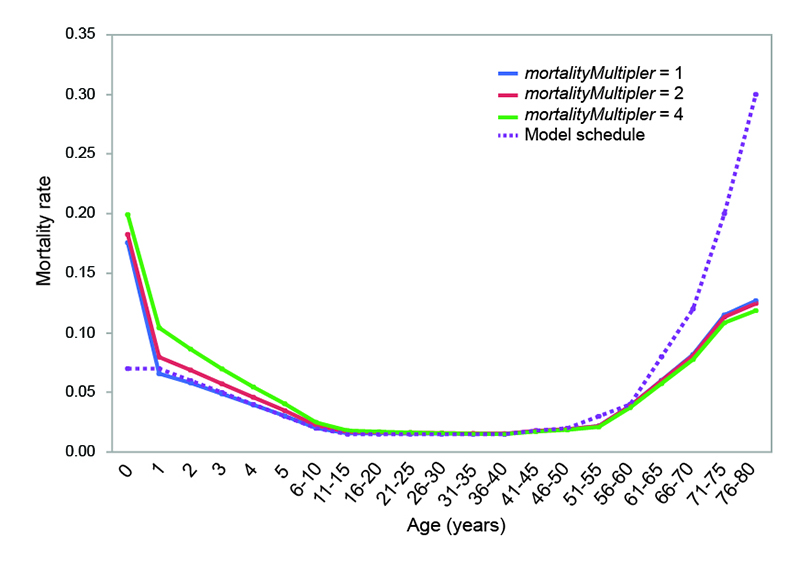
The actual patterns and values of age-specific mortality experienced by model populations are compared to the baseline schedule of probabilities used by the model in Figure 4. Under all three mortality conditions, mortality rates for individuals between 6 and 60 are nearly identical to the baseline probabilities set in the model. The economically-sensitive infanticide methods in the model produce infant mortality rates similar to those documented ethnographically (see above), and the effect is slightly greater under the more severe mortality conditions. Childhood mortality is higher than in the model schedule when the value of mortalityMultiplier is set to 2 or 4. Adults over the age of 60 experience lower mortality rates that those set by the baseline schedule in the model.
At the settings utilized in this paper, the populations in the model have relatively low fertility, high inter-birth intervals, and late mean female age at marriage compared to known ethnographic cases. In general, however, characteristics of model populations fall within ethnographic ranges. Multiple points of consistency suggest that the FN3D_V3 model reasonably captures many basic aspects of hunter-gatherer systems and is therefore a useful tool for investigating the demographic characteristics of hunter-gatherer populations and understanding how population size is related to demographic viability.
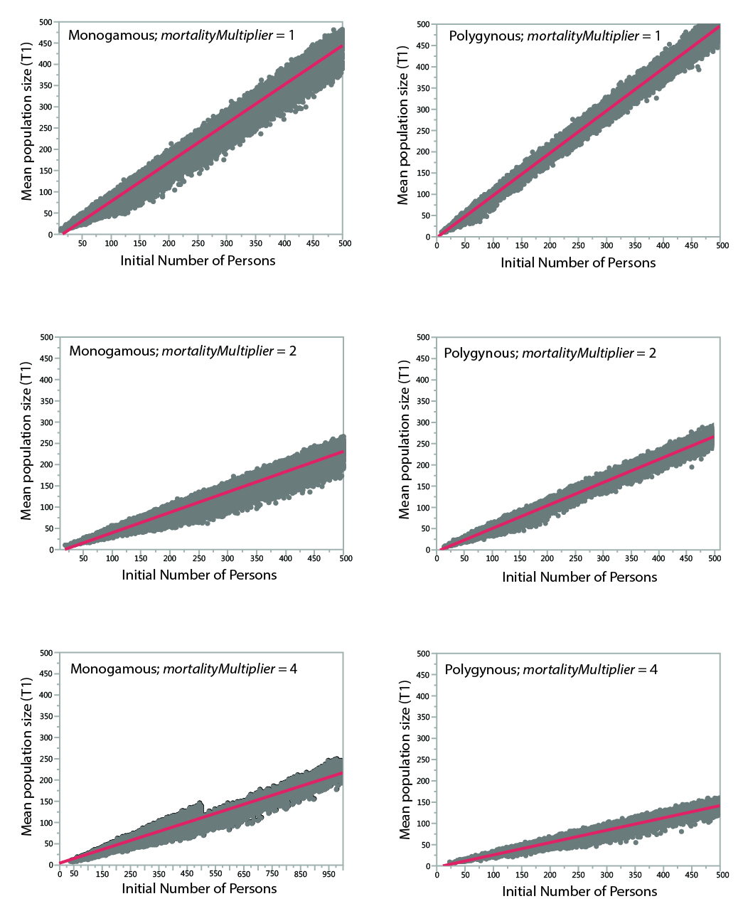
The key result of the analysis is the minimum size at which populations reliably survive a 400-year period. Although the model records the mean size of the population during a run, mean population size is a meaningless statistic for runs that go extinct. To estimate the mean population size of runs that went extinct, comparisons of initial population vs. mean population size among surviving runs were used to create a set of regression equations (Table 5). As shown in Figure 5, the relationships between initial population size and mean population size are relatively straightforward. The lower size of populations under more severe mortality conditions is apparent.
| Case | R2 | Regression Equation |
| Monogamous; mortalityMultipler = 1 | 0.977 | t1meanPopSize = -14.96665 + 0.9138677*initNumPersons |
| Polygynous; mortalityMultiplier = 1 | 0.994 | t1meanPopSize = -2.414638 + 0.9962043*initNumPersons |
| Monogamous; mortalityMultiplier = 2 | 0.970 | t1meanPopSize = -10.55064 + 0.4918262*initNumPersons |
| Polygynous; mortalityMultiplier = 2 | 0.987 | t1meanPopSize = -3.212787 + 0.542522*initNumPersons |
| Monogamous; mortalityMultiplier = 4 | 0.882 | t1meanPopSize = -3.205661 + 0.244365*initNumPersons |
| Polygynous; mortalityMultiplier= 4 | 0.960 | t1meanPopSize = -2.704945 + 0.2898954*initNumPersons |
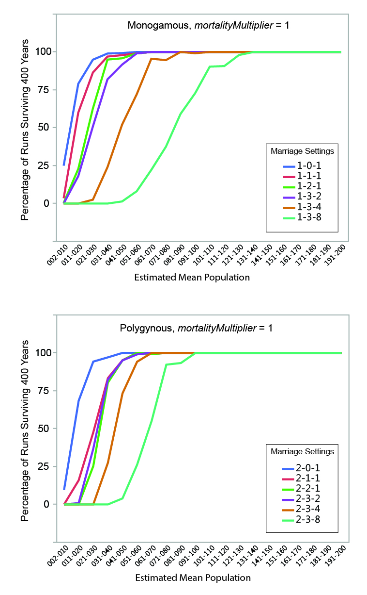
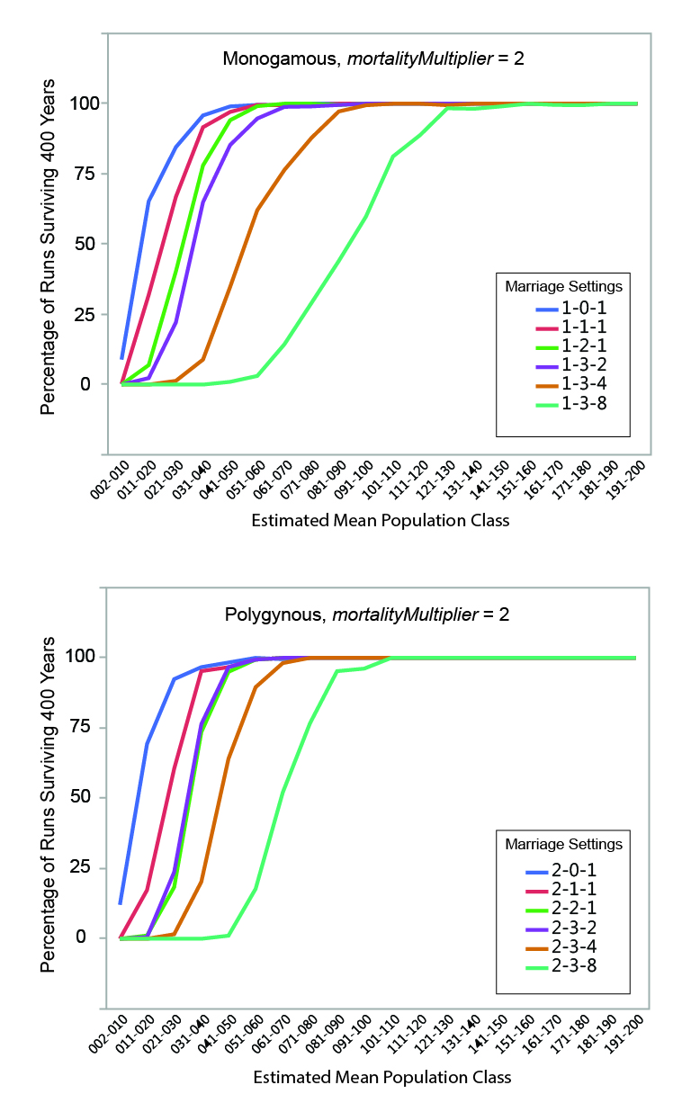
MVP size was calculated for each set of runs by determining the mean estimated population size below which fewer than 95% of the runs survived the 400-year period. The regression formulae in Table 5 were used to calculate the estimated mean population of each run from the initial population. Estimated mean population size was grouped into increments of 10 persons, and the percentage of instances where populations within a given mean size range survived (i.e., never dropped below two persons) for the full duration of a run was calculated. The relationships between estimated mean population size and survival are shown graphically in Figures 6, 7, and 8. Data are presented in summary form in Table 6.
| mortality Multiplier | Marriage settings | MVP size | Mean total fertility | Mean IBI (years) | Mean infant mortality (%) | Mean female marriage age | Mean male marriage age | Mean intensity of polygyny |
| 1 | 1-0-1 | 40 | 4.11 | 6.08 | 17.93 | 16.48 | 16.56 | 1 |
| 1 | 1-1-1 | 40 | 4.12 | 6.08 | 18.00 | 16.45 | 16.50 | 1 |
| 1 | 1-2-1 | 40 | 4.13 | 6.08 | 18.00 | 16.41 | 16.49 | 1 |
| 1 | 1-3-2 | 60 | 4.00 | 6.09 | 17.59 | 17.01 | 17.13 | 1 |
| 1 | 1-3-4 | 70 | 3.83 | 6.09 | 17.12 | 17.80 | 17.95 | 1 |
| 1 | 1-3-8 | 130 | 3.59 | 6.08 | 16.58 | 18.92 | 19.06 | 1 |
| 1 | 2-0-1 | 40 | 4.44 | 5.91 | 17.69 | 15.36 | 18.60 | 2.92 |
| 1 | 2-1-1 | 50 | 4.44 | 5.91 | 17.75 | 15.37 | 18.56 | 2.93 |
| 1 | 2-2-1 | 50 | 4.44 | 5.91 | 17.75 | 15.37 | 18.56 | 2.95 |
| 1 | 2-3-2 | 50 | 4.43 | 5.91 | 17.62 | 15.39 | 18.95 | 3.15 |
| 1 | 2-3-4 | 70 | 4.43 | 5.90 | 17.43 | 15.45 | 19.57 | 3.53 |
| 1 | 2-3-8 | 100 | 4.39 | 5.89 | 17.08 | 15.6 | 20.48 | 4.13 |
| 2 | 1-0-1 | 40 | 4.05 | 6.00 | 18.57 | 16.93 | 16.97 | 1 |
| 2 | 1-1-1 | 50 | 4.06 | 6.00 | 18.62 | 16.86 | 16.94 | 1 |
| 2 | 1-2-1 | 60 | 4.06 | 6.01 | 18.63 | 16.84 | 16.90 | 1 |
| 2 | 1-3-2 | 70 | 3.91 | 6.01 | 18.26 | 17.46 | 17.53 | 1 |
| 2 | 1-3-4 | 90 | 3.71 | 5.99 | 17.87 | 18.28 | 18.37 | 1 |
| 2 | 1-3-8 | 130 | 3.44 | 5.97 | 17.53 | 19.28 | 19.41 | 1 |
| 2 | 2-0-1 | 40 | 4.45 | 5.83 | 18.39 | 15.61 | 18.62 | 2.72 |
| 2 | 2-1-1 | 40 | 4.44 | 5.84 | 18.46 | 15.62 | 18.59 | 2.74 |
| 2 | 2-2-1 | 50 | 4.44 | 5.84 | 18.45 | 15.62 | 18.58 | 2.77 |
| 2 | 2-3-2 | 50 | 4.44 | 5.83 | 18.27 | 15.66 | 19.05 | 3.03 |
| 2 | 2-3-4 | 70 | 4.41 | 5.82 | 17.99 | 15.76 | 19.80 | 3.52 |
| 2 | 2-3-8 | 90 | 4.33 | 5.82 | 17.57 | 16.01 | 20.78 | 4.09 |
| 4 | 1-0-1 | 50 | 3.99 | 5.88 | 20.26 | 17.35 | 17.43 | 1 |
| 4 | 1-1-1 | 60 | 4.00 | 5.88 | 20.33 | 17.28 | 17.32 | 1 |
| 4 | 1-2-1 | 60 | 4.00 | 5.88 | 20.35 | 17.27 | 17.31 | 1 |
| 4 | 1-3-2 | 70 | 3.81 | 5.87 | 20.03 | 17.86 | 17.93 | 1 |
| 4 | 1-3-4 | 90 | 3.58 | 5.84 | 20.05 | 18.54 | 18.62 | 1 |
| 4 | 1-3-8 | 140 | 3.51 | 5.84 | 19.91 | 18.72 | 18.81 | 1 |
| 4 | 2-0-1 | 40 | 4.48 | 5.72 | 19.88 | 15.98 | 18.64 | 2.54 |
| 4 | 2-1-1 | 50 | 4.45 | 5.73 | 19.93 | 15.99 | 18.60 | 2.56 |
| 4 | 2-2-1 | 60 | 4.44 | 5.73 | 19.92 | 16.00 | 18.61 | 2.64 |
| 4 | 2-3-2 | 60 | 4.44 | 5.71 | 19.68 | 16.06 | 19.15 | 2.95 |
| 4 | 2-3-4 | 70 | 4.37 | 5.71 | 19.36 | 16.22 | 19.85 | 3.44 |
| 4 | 2-3-8 | 100 | 4.15 | 5.71 | 19.03 | 16.77 | 20.58 | 3.54 |

MVP sizes based on estimated mean population range from 40 to 140 (Figure 9; numeric data provided in Table 6). The data points in Figure 9 are grouped by marriage mode (monogamous and polygynous) and arranged within those modes from left to right from the "least restrictive" to the "most restrictive" marriage settings that were investigated. Unsurprisingly, the smallest MVP sizes were associated with the least restrictive marriage systems: polygynous systems with no incest taboo (pairBondMode = 2, pairBondRestrictionMode = 0, numMarriageDivisions = 1). The largest MVP sizes were associated with monogamous systems with an incest taboo and culturally-imposed marriage divisions. This is generally consistent with the idea that, other things being equal, progressively greater population sizes are required to maintain viability as cultural rules that decrease the proportion of the population suitable for marriage become more restrictive (Wobst 1974, p. 165; see also Wobst 1975).

The value of mortalityMultiplier affects MVP size in the expected way, with larger population sizes required for viability under more severe mortality conditions. The effect is most notable where MVP size is small: an increase from 40 to 60 persons (marriage setting 1-1-1, mortalityMultiplier 1 and 4), for example, represents a 50 percent increase in MVP size. In terms of the overall pattern shown in Figure 9, however, it is clear that the imposition of cultural restrictions that eliminate large portions of the population from an individual’s potential pool of mates has a greater impact on MVP size than the severity of the mortality feedback.
The imposition of an incest taboo removes closely-related persons from an individual’s pool of potential mates. Other things being equal, this would tend to increase the size of the population necessary to maintain demographic viability. In the model, the increases in population size sufficient to offset the effects of imposing a "basic" incest taboo are small in absolute terms (in the neighborhood of 10 persons). At very small population sizes, however, population changes of 10 persons are not insignificant: an increase from 40 to 50 persons increases the total population size by 25 percent.
The marriage divisions imposed by the model remove a random group of persons representing some set proportion of the population from an individual’s pool of potential mates. The imposition of marriage divisions has a significant impact on MVP size. At the most restrictive setting investigated (numMarriageDivisions = 8), population sizes required for demographic viability were 2.25 to 3.25 times larger than those with only a basic incest taboo.
Other settings being equal, polygynous systems in the model generally have smaller MVP sizes than monogamous ones. Polygynous systems are associated with higher mean total fertilities (the number of children born to a female over the course of her reproductive years), lower mean female ages at marriage, and lower mean inter-birth intervals (see Table 6 and Figure 3). The negative relationship between total fertility and female age at marriage is clear when the two variables are plotted against one another (Figure 10). The polygynous model systems provide more opportunities for females to marry earlier in life and potentially bear more offspring during the course of their reproductive spans, enhancing the viability of small populations by increasing fertility and compensating for imbalances in sex ratio. Imposition of marriage divisions has less effect on MVP size in polygynous systems than monogamous ones.

Discussion
Results from the model suggest that populations limited to as few as 40-60 people can be demographically viable over long spans of time when cultural marriage rules are no more restrictive than the imposition of a basic incest taboo. Even under the most restrictive marriage rules and most severe morality conditions imposed during model experiments, populations of at least 150 persons were demographically viable over 400 years of model time. These estimates of MVP size were calculated for populations with no logistical constraints (e.g., no impediments to information flow and no spatial component of interaction) to identifying and obtaining marriage partners.
With regard to MVP size, my results are generally consistent with the conclusions of Wobst (1974). Forty runs of his model under varying conditions returned values of MES (minimal equilibrium size) between 79 and 332 people (Wobst 1974, pp. 162-163, 166). As discussed above, Wobst’s higher, often-quoted estimate of MES range of 175-475 persons was tied to specific assumptions about both population density and the arrangement of the population in space. Neither density nor spatial distribution of population are represented in my model. It is possible that those differences alone account for the majority of differences in the results from the two models. It is also possible that differences in the representation of marriage, mortality, fertility, and family structure are important. One way to investigate this would be to implement Wobst’s model as an ABM and make a direct comparison.
Keeping in mind that MVP and MES are not strictly synonymous, the broad agreement between my results and those of Wobst is noteworthy. Both sets of results are consistent with the idea that, in the absence of strong cultural restrictions on marriage, populations limited to perhaps 150 people are of sufficient size to nearly ensure survival over long spans of time and populations limited to as few as 75 persons have a good chance of long-term survival under the same conditions.
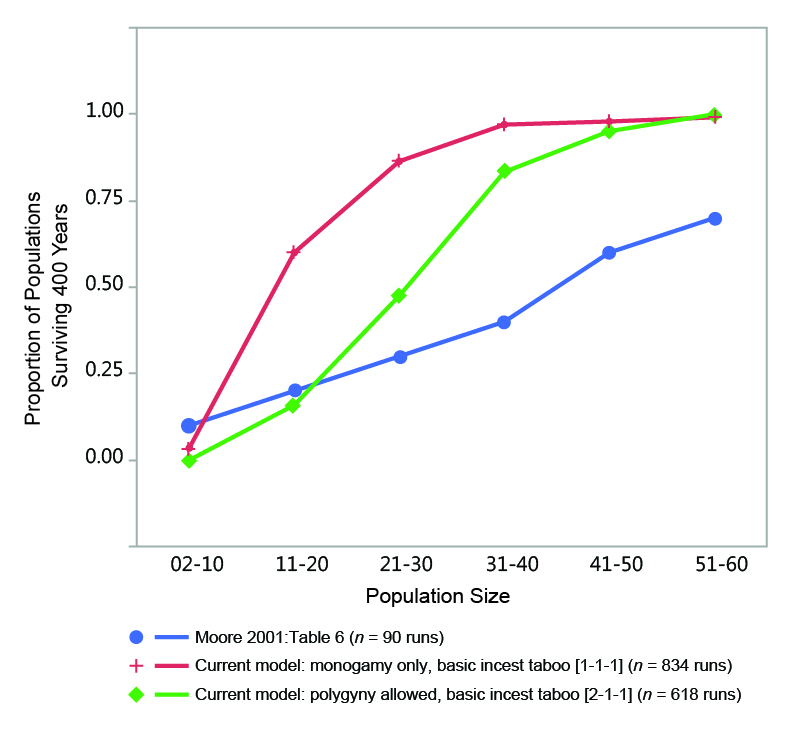
Although my conclusion is at odds with the generality offered by Moore and Moseley (2001, p. 526) that "bands of such small size [175 persons, 50 persons, or 25 persons] usually do not constitute viable mating systems that would guarantee the reproductive future of the band," it is actually in broad agreement with the data that they present. Figure 11 compares the percentage of populations of a given initial size range that survive a span of 400 years in data provided by Moore (2001, Table 6) and two sets of my own data. Moore’s (2001) results are similar to mine in terms of the relationship between initial population size and survivorship. Although Moore (2001) does not provide data for initial populations larger than 60 persons, the trends in his data clearly suggest that populations of around 100 persons would have a very high survival rate over a 400-year span in his model, even under the low fertility regime he employed to produce the results in his Table 6 (i.e., a mean of 2.56 births during a full female reproductive span; see Moore 2001, Table 1).
Thus while the details of these three models differ somewhat, their results support the general idea that human populations limited to around 100-150 persons, depending on circumstances, have a fairly high probability of survival over long periods of time in the absence of other barriers to marriage and reproduction. This applies to cases when population size is constrained by global feedbacks affecting mortality (my model) and fertility (Wobst 1974, p. 161). Under those conditions, very small populations (i.e., less than 40 people) were not viable over a 400-year period in my model.
While my results are mostly in agreement with those of previous modeling efforts, there are points of disagreement with regard to how various cultural behaviors related to marriage affect small populations. At least some of the differences between my results and those of others are probably attributable to how the models themselves function and differences in how various human behaviors are represented in the models. In the remainder of this discussion, I will discuss issues related specifically to polygyny and the incest taboo.
Polygyny
There are clear, patterned relationships between polygyny, fertility, female age at marriage, and MVP size in my results: polygynous systems in the model provide more opportunities for females to marry earlier in life and potentially bear more offspring during their finite reproductive spans. This increases mean total fertility and allows smaller MVP sizes in polygynous systems relative to monogamous ones, other conditions being the same. In very small populations, these relationships appear to enhance the probability of population survival over the long term.
As mentioned above and described in detail by White (2012, 2013, 2016b), the FN3D_V3 model uses a series of probabilistic, household-based economic calculations to determine whether or not polygynous marriage occurs in each circumstance where it is possible. These "rules" generally produce intensities of polygyny, distributions of polygynous marriage, and individual polygynous families that are verifiably like those produced by actual hunter-gatherer systems (see White 2013, pp. 157-158).
Wobst considered the effects of polygyny on his MES metric, concluding that, other things being equal, a polygynous system will tend to have a higher MES than a monogamous system because the "excess" mates available for polygynous marriage would tend to be located farther away in space (1974, pp. 157, 165-167). This conclusion is not necessarily at odds with the results I present, as I make no attempt to represent or measure the spatial extent of a marriage network. It is possible, however, that the increase in the size of the MES in polygynous systems in Wobst’s model is at least partly the result of how he represented polygynous marriage. Based on Wobst’s (1974) description, it is not clear exactly how polygynous marriage was operationalized in his model. The size and composition characteristics of the families produced by Wobst’s representation of polygynous marriage are likewise unknown.
Moore’s model represented polygyny "simply by allowing married men to remain in the marriage pool" (Moore 2001, p. 398), apparently subject to the same risk of marriage as unmarried males. He does not provide data which allow comparisons of the behavior of monogamous and polygynous systems in his model. As with Wobst’s (1974) model, the size and composition characteristics of the families produced by Moore’s representation of polygynous marriage are unknown.
The relationship between total fertility and the percentage of polygynous marriage in the model results is interesting in light of the available ethnographic data. While the issue has been a contentious one (see Borgerhoff Mulder 1989; Dorjahn 1958; Isaac 1980; Josephson 2002), the majority of studies suggest that polygynous marriage is associated with decreased fertility relative to monogamous marriage (e.g., Dorjahn 1958; Hern 1992; Isaac 1980; but also see Barber 2004). Several mechanisms have been proposed to explain this apparent negative relationship, none of which has been shown to be a sufficient explanation in a large number of cases: it is clear that the relationship between polygyny and fertility is not simple across the spectrum of ethnographic cases for which we have data (Josephson 2002).
The same can also be said for the model systems considered here. Figure 11 shows mean total fertility rates, mean inter-birth intervals, and mean infant mortality rates for polygynous populations under all three mortality settings (data points from runs with less than 10 percent and greater than 40 percent polygyny are not shown, as sample sizes for those categories are very small). Between about 15-35 percent polygynous marriage, all three mortality conditions show a general pattern of decreasing fertility (Figure 12a). Mean inter-birth interval generally decreases through this range (Figure 12b). The relationship between infant mortality and the percentage of polygyny is more complicated, as the general pattern appears to differ by mortality condition (Figure 12c). Infant mortality and inter-birth interval appear to be affected by differences in overall mortality regime (i.e., the value of mortalityMultiplier) to a much greater degree than total fertility.

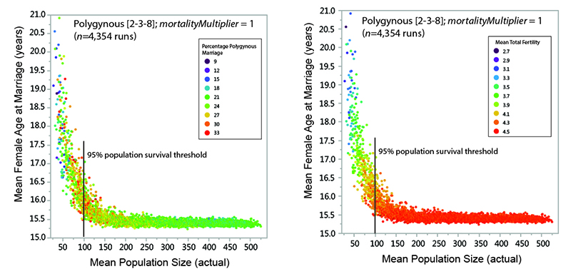
As explained above, fertility rates in the model appear to be strongly related to the proportion of the female reproductive span that is spent in marriage (i.e., in a state where reproduction is possible). Considering a subset of the model data allows us to consider the how female marriage age and polygyny are related to MVP size. Figure 13 shows data from surviving populations in one set of experiments (polygynous system, mortalityMultiplier = 1; eight marriage divisions). There is a strong non-linear relationship between mean population size and the mean age at which females were married, with far greater variability in marriage age in populations below the threshold of demographic viability (in this case, around 100 persons). There is also much greater variability in the percentage of polygynous marriage among populations below the viability threshold (Figure 13a) and a strong relationship between mean female age at marriage and mean total fertility (Figure 13b). The idea that the demographic outcomes of model systems with small populations are characterized by a much wider range of variability (in terms of variables such as polygyny and fertility) than systems with larger populations is generally consistent with earlier explorations of the sensitivities of the model (White 2016a). As population size decreases, stochastic variability increases in importance: the demographic characteristics of the population are more sensitive to each individual birth, death, and marriage. Other things being equal, female age at marriage is perhaps the most important variable affecting fertility in small populations in the model.
Overall, results from the model suggest that polygynous marriage may be an important mechanism for increasing the viability of small hunter-gatherer systems by lowering the mean female age at marriage (and increasing mean fertility) when there is an imbalance in the number of available males and females of marriageable age. Because no attempt is made to represent many of the linkages between polygynous marriage and fertility that have been suggested as explanations for decreased fertility in polygynous societies (e.g., the "dilution effect" of polygynous men sharing their reproductive output among multiple women, female sterility as an incentive for multiple marriage, conflict between co-wives, and age-based changes in fecundity – see Josephson 2002), we can be sure that none of these factors is responsible for the behavior seen in the model.
Marriage restrictions based on the incest taboo
Results from the experiments suggest that relaxing prohibitions on marriage among close kin has a small effect on MVP size. The significance of this effect is greatest at small population sizes, where each individual is a larger proportion of the total population. As with polygyny, relaxing prohibitions on incestuous marriage has the effect of increasing the number of potential mates within a population of a given size, potentially lowering the mean female age at marriage and mitigating an imbalance in the numbers of marriageable males and females.
My results are generally consistent with those of Wobst (1974, pp. 165-166), who found little to no difference in the size of the MES when the incest taboo was removed. Another modeling effort by Wobst (1975) supported the idea that imposition of an incest taboo in a small population (i.e., 100 individuals) required a significant increase in fertility to prevent that population from going extinct. An increase in fertility among married females was necessary to compensate for the fertility lost by females who were of reproductive age but not married because of a lack of available mates (Wobst 1975, p. 79).
Some of my results are at odds with the assertions of Moore (2001) and Moore and Moseley (2001) regarding the idea that marriage prohibitions based on incest taboos would pose a significant threat to the viability of small colonizing populations:
"The marriage problem is generated by the fact that foraging bands, of perhaps 25 to 50 persons each, are conventionally organized around a coresident lineage...so that potential spouses in a band – people of opposite sex but similar ages...are closely related to each other and cannot marry" (Moore 2001:397).
My results suggest that very small initial populations with an incest taboo can reliably survive under the right circumstances (i.e., if polygyny is permitted and fertility is high enough). Ethnographic information suggests two additional reasons to be skeptical of the idea that incest taboos would prevent small foraging bands from being viable founding populations. First, the idea that foraging bands are composed mainly of closely related individuals is not supported by recent ethnographic data: "close" kin accounted for less than 10 percent of the membership of the sample of hunter-gatherer groups considered by Hill et al. (2011). This is consistent with the high degree of flux in group membership noted for many ethnographic hunter-gatherers (e.g., see Binford 2001; Kelly 1995; Lee and DeVore 1968, p. 7; Marshall 1976, pp. 179-180; Silberbauer 1981; Turnbull 1968; Woodburn 1968), which would tend to produce foraging groups that contained individuals not necessarily related by close kinship.
Second, while marriage rules specifying who may and may not marry exist in all human cultures, actual behavior can, and often does, deviate from those rules. Individuals within the system often do not follow the "rules", and rules exist (or can be created) to circumvent the "rules" (Keesing 1975, p. 83; Kelly 1995, p. 286; see also Buchler and Selby 1968; Murdock 1965). Ecological, demographic, and economic circumstances can produce different kinship and marriage behaviors within the same set of "rules" (e.g., Keesing 1975, pp. 123, 135). We might suspect, then, that strict marriage restrictions based on incest taboos could be relaxed when small, isolated populations are demographically stressed, such as during a “stochastic crisis” associated with colonization.
Conclusion
In this paper, I have attempted to isolate the effects of marriage behaviors on the size of demographically viable populations. In real hunter-gatherer systems, obviously, numerous other conditions, behaviors, and characteristics (none of which exist in a vacuum) are potentially related to demographic viability. Other recent modeling efforts have focused on issues such as cooperation, cultural transmission, subsistence economics, and mobility (e.g., see Barceló and Del Castillo 2016; Lewis et al. 2014; Santos et al. 2015; White 2013). As model-based efforts continue to develop, it will be possible to build theory linking together these various characteristics and dynamics of hunter-gatherer systems.
The experimental framework utilized here suggests that, under many circumstances, a population of about 150 persons is of sufficient size to be considered demographically viable over a long span of time. Out of a total of 67,614 runs with mean estimated populations over 150, only nine went extinct. Female age at marriage appears to be a key variable influencing MVP size: fewer cultural restrictions on marriage behaviors are linked to lower female ages at marriage, increased fertility, and lower MVP sizes.
My results are broadly consistent with those from two other models (Moore 2001 and Wobst 1974) that have considered questions of demographic viability and accord reasonably well with the empirical data we have that documents the existence of hunter-gatherer social systems appreciably smaller than 500 persons (see Birdsell 1953, Figure 9; Moffett 2013). Factors other than stochasticity in mortality, fertility, and sex ratio (e.g., environmental variability of spatial components of interaction behaviors) presumably influence the size of actual hunter-gatherer social systems and encourage them to exceed the minimum size threshold required for demographic viability. If we accept that a population of 150 is a reasonable baseline estimate for the population size sufficient to ensure demographic viability over long spans of time, we might then reasonably reconsider our explanations for why some hunter-gatherer social systems exceed this minimum. If there is a downward pressure that encourages hunter-gatherer social systems to be as small as possible, it seems likely that something other than demographic viability (in the sense of the term as used here) constitutes the limiting factor when social systems encompass significantly more than 150 people. Understanding how other factors might relate to the minimum and maximum size of hunter-gatherer populations will require further work.
While this analysis wasn’t aimed directly at issues of the viable size of colonizing populations, it is worth noting that the results do not necessarily conflict with the idea that successful colonizing populations of hunter-gatherers could initially be much smaller than MVP size. The experiments discussed here were performed under conditions where population sizes were stabilized through a feedback mechanism to determine at what population threshold the inherent stochastic variability in human mortality/fertility was not a threat to long-term survival. In the absence of feedbacks to constrain population size, conditions where fertility exceeds mortality could allow very small populations to grow to a point where normal stochastic perturbations no longer pose a threat of extinction. Exploration of that subject will require further experimentation.
The analysis presented here could be expanded in several additional directions. Parameterized representation of spatial and/or temporal limitations to marriage opportunities, for example, could be used to investigate the effects of the scales and rhythms of population aggregations on MVP size. Experimentation with the age at which individuals are eligible to marry could be used to analyze the effects of cultural rules that proscribe marriage age and differences in those rules for males and females. A more nuanced approach to the imposition of marriage divisions could be taken to more closely represent the rules of the moiety structures that have been documented ethnographically. In all cases, the default hypothesis is that rules and behaviors that potentially limit access to marriage partners will tend to increase MVP size. Whether any reasonable mechanisms that that constrain marriage will be able, alone or in combination, to increase MVP size to the “magic number” of 500 is a question to be addressed by future systematic investigation.
Acknowledgements
Many components of the model used in this analysis were constructed during my doctoral work at the University of Michigan. Bob Whallon, John Speth, Henry Wright, and Rick Riolo served both as dissertation committee members and sources of clarity and perspective during that effort. Two anonymous reviewers commented constructively on an earlier draft of this paper. I am responsible for any and all errors.References
BARBER, N. (2004). Sex ratio at birth, polygyny, and fertility: A cross-national study. Social Biology, 51(1/2), 71-77. [doi:10.1080/19485565.2004.9989084]
BARCELÓ, J. A., & Del Castillo, F. (Eds.) (2016). Simulating Prehistoric and Ancient Worlds. Cham: Springer International. [doi:10.1007/978-3-319-31481-5]
BETZIG, L. L. (1986). Despotism and Differential Reproductive Success: A Darwinian View of Human History. Chicago: Aldine.
BINFORD, L. R. (1980). Willow smoke and dog’s tails: hunter-gatherer settlement systems and archaeological site formation. American Antiquity, 45(1), 4-20. [doi:10.2307/279653]
BINFORD, L. R. (1983). 'Long term land use patterns: some implications for archaeology.' In R. C. Dunnell & D. K. Grayson (Eds.), Lulu Linear Punctated: Essays in honor of George Irving Quimby (pp. 27-53). Anthropological Papers No. 72, Museum of Anthropology, University of Michigan.
BINFORD, L. R. (2001). Constructing Frames of Reference: An Analytical Method for Archaeological Theory Building Using Hunter-Gatherer and Environmental Data Sets. Berkeley: University of California Press.
BIRDSELL, J. B. (1953). Some environmental and cultural factors influencing the structuring of Australian aboriginal populations. The American Naturalist, 87(834), 171-207. [doi:10.1086/281776]
BIRDSELL, J. B. (1958). On population structure in generalized hunting and collecting populations. Evolution, 12(2), 189-205. [doi:10.1111/j.1558-5646.1958.tb02945.x]
BIRDSELL, J. B. (1968). 'Some predictions for the Pleistocene based on equilibrium systems among recent hunter-gatherers.' In R. B. Lee & I. DeVore (Eds.), Man the Hunter (pp. 229-240). Chicago: Aldine.
BORGERHOFF MULDER, M. (1989). Marital status and reproductive performance in Kipsigis women: Re-evaluating the polygyny-fertility hypothesis. Population Studies, 43, 285-304. [doi:10.1080/0032472031000144126]
BUCHLER, I. R., & Selby, H. A. (1968). Kinship and Social Organization. New York: Macmillan.
DORJAHN, V. R. (1958). Fertility, polygyny and their interrelations in Temne society. American Anthropologist, 60, 838-860. [doi:10.1525/aa.1958.60.5.02a00050]
GILBERT, N. (2008). Agent-Based Models. Thousand Oaks: Sage Publications. [doi:10.4135/9781412983259]
GURVEN, M., & H. Kaplan (2007). Longevity among hunter-gatherers: A cross-cultural examination. Population and Development Review, 33, 321-356. [doi:10.1111/j.1728-4457.2007.00171.x]
HAMILTON, M. J., Milne, B. T., Walker, R. S., Burger, O., & Brown, J. H. (2007). The complex structure of hunter-gatherer social networks. Proceedings of the Royal Society B, 274, 2195-2202. [doi:10.1098/rspb.2007.0564]
HELM, J. (1965). Bilaterality in the socio-territorial organization of the Arctic Drainage Dene. Ethnology, 4, 361-385. [doi:10.2307/3772786]
HERN, W. M. (1992). Polygyny and fertility among the Shipibo of the Peruvian Amazon. Population Studies, 46, 53-64. [doi:10.1080/0032472031000146006]
HEWLETT, B. S. (1991). Demography and childcare in preindustrial societies. Journal of Anthropological Research, 47(1), 1-37. [doi:10.1086/jar.47.1.3630579]
HILL, K., & Hurtado, A. M. (1996). Ache Life History: The Ecology and Demography of a Foraging People. New York: Aldine de Gruyter.
HILL, K., Hurtado, A. M., & Walker, R. S. (2007). High adult mortality among Hiwi hunter-gatherers: Implications for human evolution. Journal of Human Evolution, 52, 443-454. [doi:10.1016/j.jhevol.2006.11.003]
HILL, K. R., Walker, R. S., Božičević,, M., Eder, J., Headland, T., Hewlett, B., Magdalena Hurtado, A., Marlowe, F., Wiessner, P., & Wood, B. (2011). Co-residence patterns in hunter-gatherer societies show unique human social structure. Science, 331, 1286-1289. [doi:10.1126/science.1199071]
HOWELL, N. (1979). Demography of the Dobe !Kung. New York: Academic Press.
ISAAC, B. L. (1980). Female fertility and marital form among the Mende of rural Upper Bambara Chiefdom, Sierra Leone. Ethnology,19(3), 297-313. [doi:10.2307/3773334]
JARVENPA, R., & Brumbach, H. J. (1988). Socio-spatial organization and decision-making processes: observations from the Chipewyan. American Anthropologist, 90, 598-618. [doi:10.1525/aa.1988.90.3.02a00050]
JOSEPHSON, S. C. (2002). Does polygyny reduce fertility? American Journal of Human Biology, 14, 222-232. [doi:10.1002/ajhb.10045]
KEEN, I. (2004). Aboriginal Economy and Society: Australia at the Threshold of Colonisation. Oxford: Oxford University Press.
KEEN, I. (2006). Constraints on the development of enduring inequalities in Late Holocene Australia. Current Anthropology, 47(1), 7-38. [doi:10.1086/497672]
KEESING, R. M. (1975). Kin Groups and Social Structure. New York: Holt, Rhinehart and Winston.
KELLY, R. L. (1995). The Foraging Spectrum. Washington, D.C.: Smithsonian Institution Press.
LEE, R. B. (1984). The Dobe !Kung. Fort Worth: Harcourt Brace College Publishers.
LEE, R. B., & DeVore, I. (Eds.). (1968). Man the Hunter. Chicago: Aldine.
LEWIS, H. M., Vinicius, L., Strods, J., Mace, R., & Migliano, A. B. (2014). High mobility explains demand sharing and enforced cooperation in egalitarian hunter-gatherers. Nature Communications 5, 5789. [doi:10.1038/ncomms6789]
LEWIS-WILLIAMS, J. D. (1982). The economic and social context of southern San rock art. Current Anthropology, 23, 429-449. [doi:10.1086/202871]
MARSHALL, L. (1976). The !Kung of the Nyae Nyae. Cambridge: Harvard University Press. [doi:10.4159/harvard.9780674180574]
MEGGITT, M. J. (1968). '"Marriage classes" and demography in central Australia.' In R. B. Lee & I. DeVore (Eds.), Man the Hunter (pp. 176-184). Chicago: Aldine.
MOFFETT, M. W. (2013). Human identity and the evolution of societies. Human Nature, 24(3), 219-267. [doi:10.1007/s12110-013-9170-3]
MOORE, J. H. (2001). Five models of human colonization. American Anthropologist, 103(2), 395-408. [doi:10.1525/aa.2001.103.2.395]
MOORE, J. H., &; Moseley, M. E. (2001). How many frogs does it take to leap around the Americas? Comments on Anderson and Gillam. American Antiquity, 66(3), 526-529. [doi:10.2307/2694250]
MURDOCK, G. P. (1965) [1949]. Social Structure. New York: The Free Press.
MURDOCK, G. P. (1967). Ethnographic Atlas: A summary. Ethnology, 6,109-236. [doi:10.2307/3772751]
PENNINGTON, R. (2001). 'Hunter-gatherer demography.' In C. Panter-Brick, R. H. Layton, & P. Rowley-Conwy (Eds.), Hunter-Gatherers: An Interdisciplinary Perspective (pp. 170-204). Cambridge: Cambridge University Press.
SAKAI, A. K., Allendorf, F. W., Holt, J. S., Lodge, D. M., Molofsky, J., With, K. A., Baughman, S., Cabin, R. J., Cohen, J. E., Ellstrand, N. C., McCauley, D. E., O’Neil, P., Parker, I. M., Thompson, J. N., & Weller, S. G. (2001). The population biology of invasive species. Annual Review of Ecology and Systematics, 32, 305-332. [doi:10.1146/annurev.ecolsys.32.081501.114037]
SANTOS, J. I., Pereda, M., Zurro, D., Álvarez, M., Caro, J., Galán, J. M., & Briz, I. (2015). Effect of resource spatial correlation and hunter-fisher-gatherer mobility on social cooperation in Tierra del Fuego. PLoS ONE, 10(4). [doi:10.1371/journal.pone.0121888]
SHAFFER, Mark L. (1981). Minimum population sizes for species conservation. BioScience, 31(2), 131-134. [doi:10.2307/1308256]
SILBERBAUER, G. B. (1981). Hunter and Habitat in the Central Kalahari Desert. Cambridge: Cambridge University Press.
TURNBULL, C. M. (1968). 'The Importance of Flux in two Hunting Societies.' In R. B. Lee & I. DeVore (Eds.), Man the Hunter (pp. 132-137). Chicago: Aldine.
WHITE, A. A. (2012). The Social Networks of Early Hunter-Gatherers in Midcontinental North America. Unpublished Ph.D. Dissertation: University of Michigan.
WHITE, A. A. (2013). Subsistence economics, family size, and the emergence of social complexity in hunter-gatherer systems in eastern North America. Journal of Anthropological Archaeology, 32(2), 133-163. [doi:10.1016/j.jaa.2012.12.003]
WHITE, A. A. (2016a). 'The sensitivity of demographic characteristics to the strength of the population stabilizing mechanism in a model hunter-gatherer system.' In M. Brouwer Burg, H. Peeters, and W. Lovis (Eds.), Uncertainty and Sensitivity Analysis in Archaeological Computational Modeling (pp. 113-130). Cham: Springer International. [doi:10.1007/978-3-319-27833-9_7]
WHITE, A. A. (2016b). ForagerNet3_Demography_V3 (Version 1). CoMSES Computational Model Library. http://www.openabm.org/model/5300/version/1.
WHITE, P. C. L., Ford, A. E. S., Cloud, M. N., Engeman, R. M., Roy, S., & Saunders, G. (2008). Alien invasive vertebrates in ecosystems: Pattern, process and the social Dimension. Wildlife Research, 35(3), 171-179. [doi:10.1071/WR08058]
WOBST, M. H. (1971). Boundary Conditions for Paleolithic Social Systems: A Simulation Approach. Unpublished Ph.D. Dissertation: University of Michigan.
WOBST, M. H. (1974). Boundary conditions for Paleolithic social systems: A simulation approach. American Antiquity, 39(2-Part1), 147-178. [doi:10.2307/279579]
WOBST, M. H. (1975). The demography of finite populations and the origins of the incest taboo. Population Studies in Archaeology and Biological Anthropology: A Symposium. Memoirs of the Society for American Archaeology, 30, 75-81.
WOODBURN, J. (1968). 'Stability and flexibility in Hadza residential groupings.' In R. B. Lee & I. DeVore (Eds.), Man the Hunter (pp. 101-110). Chicago: Aldine.
YELLEN, J., & Harpending, H. (1972). Hunter-gatherer populations and archaeological inference. World Archaeology, 4(2), 244-253. [doi:10.1080/00438243.1972.9979535]
YENGOYAN, A. A. (1968). 'Demographic and ecological influences on aboriginal Australian marriage sections.' In R. B. Lee & I. DeVore (Eds.), Man the Hunter (pp. 185-199). Chicago: Aldine.