
Introduction
Microsimulations and agent-based models (ABMs) are increasingly used across a broad area of disciplines, e.g. biology (Gras et al. 2009), sociology (Macy et al. 2002), economics (Deissenberg et al. 2008) and epidemiology (Gray et al. 2011) . In many of these applications an artificial society of agents, usually representing humans or animals, is created, and the agents need to be paired with each other to allow for interactions between them.
Zinn (2012) addresses some of the conceptual challenges of finding suitable pairs of agents, particularly with respect to closed continuous ABMs. The author differentiates between stochastic versus stable matching rules, discusses different measures of compatibility between agents (which we call distance functions) and which agents choose their partners and which only get chosen. While the paper provides a conceptual framework of matching procedures, computational algorithmic aspects are left out and little research can be found on this topic. Bouffard et al. (2001) presents an algorithm for finding suitable pairs for marriage. However this algorithm would be too slow for the repeated pair-matching required in many microsimulations of sexually transmitted infections (STIs).
The identification of suitable pairs of agents for partnerships may be difficult to compute efficiently. If a simulation does not measure the compatibility of two agents, i.e. it assumes that agents behave uniformly and match randomly with one another, then it risks failing to model essential features that determine the outcomes being studied.
On the other hand if a model attempts to measure the compatibility of agents, so that it produces sets of agent partnerships that very closely match the population being studied, it may become too computationally slow to study large populations; it may even be too slow for small populations where agents seek new partners repeatedly. The choice of pair-matching algorithm therefore needs to consider the trade-off between accuracy and speed to ensure the feasibility of the microsimulation for the research question at hand. This is especially true if the model is stochastic and needs to be run many times for the construction of confidence intervals or sensitivity analyses.
Two algorithms are commonly used for pair-matching in microsimulations. One randomly matches agents in a mating pool into pairs. While this does not usually yield good quality matches with respect to the actual distribution of partnerships in the population being studied, it is fast: the time of the pair-matching procedure is linear with the number of agents being matched.
The second algorithm is a brute force approach (using common computer science terminology, e.g. Levitin (2011). This algorithm compares each agent to every other unmatched agent in the mating pool, using a compatibility or distance function, in order to choose appropriate partnerships. While this method usually yields good quality matches, it is slow, with execution time quadratic with the number of agents being matched.
The aim of our study is to present several alternative pair-matching algorithms for microsimulations and ABMs, which allow for a better trade-off between good quality matches and computation time than the random and brute-force methods. After the general problem statement and a description of general characteristics of pair-matching algorithms, we provide a detailed description of the matching algorithms. As this paper focuses on the computational features, we analyse the respective relative efficiency and effectiveness of the algorithms compared to brute force and random matching algorithms for one abstract microsimulation, and one microsimulation that models some features of a natural population in the field of epidemiology.
We have provided open-source C++ implementations of the algorithms, although modellers will likely wish to adapt them for their domains. We hope that these algorithms will lead to faster more accurate, easier-to-implement microsimulations, especially, but not only, of STI epidemics.
Background
General problem statement
The typical structure of a discrete microsimulation or ABM is that the simulation is divided into time steps, and in each time step events execute over all the agents. For example, see Algorithm 1.
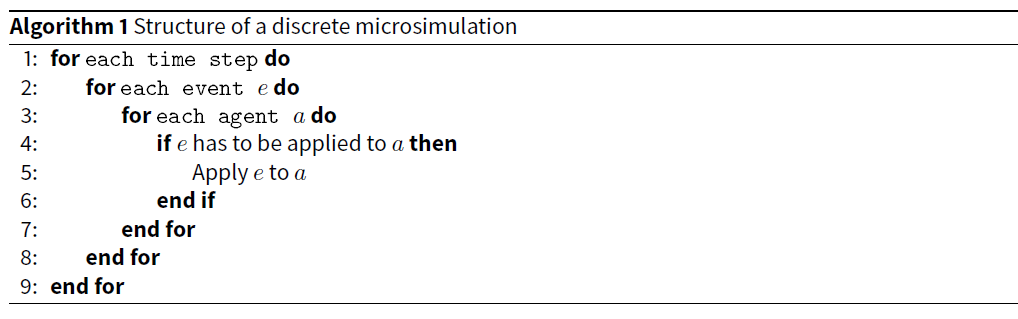
The practicability of a simulation is dependent on the efficiency of the events. A particularly simple event is to age each agent. This merely requires incrementing an age property for each agent. The execution time is linear with the number of agents. We usually want the efficiency class of events to be linear, or at worst linearithmic (i.e. the execution time is proportional to n log n, where n is the number of agents being matched). An event whose time efficiency is quadratic (n2) with the number of agents being matched will slow simulations with large numbers of agents to the point that it may become unfeasible to generate confidence intervals or conduct sensitivity testing.
Pair-matching represents a more complex event involving the properties of more than one agent and can be stated formally as follows: We have a set of n agents eligible for pairing a1, a2…an. We have a distance function distance which takes two agents as its parameters such that if distance(a,b) < distance(a,c) then b is a more likely, compatible, suitable or appropriate match for a than c. (If it is possible that distance (a, b) = distance(a,c) the modeller must decide on a tie-breaking mechanism.) A pair-matching solution is a set of matches such that every agent is paired with exactly one other agent. This can be recast as a fully-connected graph problem such that every vertex is an agent and every edge is a distance between two agents.
There exists for such a graph with n vertices multiple sets of distinct pair-matchings. One or more of these is a minimum-distance — or perfect — set in that the sum of all the distances between the pairs is less than or equal to every other pair-matching set. There are algorithms that find the minimum-distance set of pair-matchings, such as Blossom V (Kolmogorov 2009; Cook & Rohe 1999). However, Blossom V suffers from two serious problems: it is far too slow for most microsimulations, and it is not stochastic — it always produces the same set of pairs, unless there are multiple perfect pair-matching sets, in which case the algorithm could be modified to produce a random tie-breaking mechanism. Usually, though, more stochasticism than this is required. Nor is reproducing the expected value of a probabilistic distribution with certainty usually a desirable statistical attribute of a microsimulation.
Instead we are interested in pair-matching algorithms that approximate the underlying distribution, and do so quickly. This paper presents several such pair-matching algorithms, some of them novel. They are tested, compared and analysed, including against the Blossom V algorithm.
Characteristics of pair-matching algorithms
Pair-matching algorithms may be described and categorized in general by the following characteristics:
Distance function If agents are not matched randomly, a distance function must be defined. This function indicates the compatibility of a pair of agents for a partnership based on the distribution of partnerships in the population being modelled, as described in 2.3.
Exact vs approximate In some applications, agents are only paired if they are an exact match, i.e. for two agents a and b, they are paired if and only if distance(a, b) equals a defined value. In other applications, only an approximate match is necessary. In this paper the algorithms are compared using approximate matching applications. Nevertheless, the algorithms can all be adapted to do either approximate or exact matching.
Stochasticism Stochasticism in partner choice is usually desired in microsimulations, for example so that multiple executions of the simulation differ from each other. As agents are usually stored in an array data structure, or similar, pair-matching algorithms will process the array from front to back. If the agents that are processed first are more likely to find compatible partners than those processed last, as the pair-matching event is repeated in subsequent time-steps, the partner selections will become increasingly biased. An easy way to avoid this ”storage” bias is through the introduction of randomness by shuffling agents using the technique described in Knuth (1997, pp.142-146) and that is implemented in most modern programming language standard libraries. Further randomness can be introduced if desired. For example, the maximum number of evaluated potential matching candidates or the threshold of the value of the distance function for accepting partners may be stochastic.
Effectiveness We call an algorithm’s success at generating matches its effectiveness. We evaluate this using two measures. When exact matching is used, the first effectiveness measure is calculated as the proportion of the agent population, who are supposed to be in relationships, that are actually in relationships after the algorithm is executed across all agents. For approximate matching, effectiveness is the mean or median distance between all paired agents. The second effectiveness measure is defined as follows: For any agent a we can rank all other agents in order of distance from a. Then the effectiveness is the mean or median rank of all agent partners. Both measures are relative, if the best possible matching result is unknown (because it is too computationally demanding to calculate).
Initialisation vs in-simulation All the pair-matching algorithms discussed here are intended for execution as events during a simulation as in Algorithm 1. However, in some simulations, it is necessary to pair agents before the simulation starts. An example of an algorithm to do this is discussed in Scholz et al. (2016).
Distance functions
Euclidean distance would be a convenient measure of the suitability of pairing two agents a and b with m appropriately scaled properties a1, b1, a2, b2… am, b m. For multi-dimensional space, the equation for Euclidean distance is:
| $$d(a,b)=\sqrt{(a_1-b_1)^2+(a_2-b_2)^2+...+(a_m-b_m)^2}$$ |
Algorithms exist that efficiently but approximately find the nearest neighbour to a point in high-dimensional Euclidean space (Indyk & Motwani 1998; Beis & Lowe 1997; Arya et al. 1998). It is unclear how easily these can be adapted to microsimulations, but perhaps if we could map the properties of agents to Euclidean space, we could use one of these algorithms (or a variation thereof) to find suitable partners.
To map the matching properties to metric space, of which Euclidean space is one example, the distance function would have to satisfy the triangle inequality (Weisstein 2016). For agents a, b and c this is:
| $$distance(a,b) + distance(b,c) \geq distance(a,c)$$ |
In some simulations the agent properties violate the triangle inequality. An example is the primarily heterosexual HIV epidemic in South Africa. Consider the agent properties we are interested in for measuring pairing suitability:
- age
- sex
- desire for a new partnership at this time
- risk behaviour propensity (including whether or not the agent is a sex worker)
- relationship status (including whether or not the agent is married)
- location
The more similar two individuals the closer they are to each other in Euclidean space, but this is not the case for heterosexual agents in an HIV epidemic: If two people share the same sex they are not suitable partners in this model. See Figure 1 for a graphical depiction of how this violates the triangle inequality.
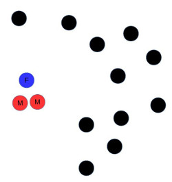
The problem is not confined to modelling heterosexual relationships. Even if we want to model only men who have sex with men (MSM) with respect to an STI, it would be difficult to map our agents to Euclidean space. We might want our microsimulation to make it less likely for married agents seeking a new partnership to partner with other married agents, or with other agents currently in a relationship. When searching for a new relationship, we might want the distance to be great between otherwise well-matched agents who have been in a partnership with each other previously. We might also want to extend our model to account for people looking for partners of different age, wealth or education from themselves.
In our model’s set of agent properties, age, risk behaviour propensity and geographical location may be attributes that map well to Euclidean space; we could define our distance function so that the more similar these are between agents, the more likely they are to form partnerships. However, sex for heterosexual agents does not map to Euclidean space, and, depending on the model’s assumptions, neither might several other agent attributes. (While it might be argued that sexual orientation is a categorical variable, a distance function simply returns a real number, and therefore has to represent incompatible categories of agents by calculating a very high value for such pairs of agents.)
We call a model’s agent properties which do map well to Euclidean space attractors, and attributes that do not rejectors. Two of the algorithms we present (CSPM and WSPM) work by clustering agents together based on their attractors. Therefore clustering functions have to be defined by modellers who use these algorithms. However, when the rejectors dominate the distance function, the cluster function is less useful and the effectiveness of these two algorithms degrades.
Pair-matching algorithms
Besides the above mentioned Brute force pair-matching (BFPM) and Random pair-matching (RPM) algorithms, we describe the following four pair-matching algorithms.
- Random k pair-matching (RKPM)
- Weighted shuffle pair-matching (WSPM)
- Cluster shuffle pair matching (CSPM)
- Distribution counting pair-matching (DCPM)
Brute force pair-matching (BFPM)
This algorithm works as follows: For every agent a in a set of agents, it calculates the distance to every remaining unpaired agent after a in the set. The agent b with the smallest distance to a is marked as a’s partner (and vice-versa).
This is a naive algorithm that is very effective. However, unless pair matching only needs to be executed a few times, or on small populations, it is impractically slow — quadratic with the number of agents being paired. For example to run one simulation of a subset of the South African population to model the HIV epidemic for five years, we iterate over tens of thousands of agents daily or weekly, executing pair-matching on each iteration. Numerous simulations need to be run in order to build confidence intervals or to perform sensitivity testing (see for example Hontelez et al. 2013 and Johnson & Geffen 2016). The BFPM algorithm is usually too slow for this purpose.
As BFPM, or variations thereof, is widely implemented in microsimulations and ABMs, we use it here as a reference against which to measure the effectiveness and speed of the other algorithms.
The pseudocode for BFPM is provided in Algorithm 2.

Random pair-matching (RPM)
Many deterministic models that use differential equations to model population dynamics or epidemiology, as well as simple microsimulations make the simplifying assumption that people are randomly paired with their sexual partners. This corresponds to a random matching algorithm using no distance function. Although this is extremely fast, with execution speed linear with the number of agents being matched, by ignoring the compatibility of matched agents it may result in the simulation producing outputs that differ wildly from the population being modelled.
As with BFPM, this algorithm’s primary purpose is as a yardstick against which to measure the other algorithms. A good algorithm will execute much faster than BFPM but perhaps considerably slower than RPM. The effectiveness of a good algorithm should far exceed RPM. Algorithm 3 presents the pseudocode for this algorithm.

Random k pair-matching (RKPM)
This algorithm is a small conceptual advance on RPM and BFPM (Pelillo 2014; Larose & Larose 2014). Instead of only considering all agents following a, the one under consideration (as in BFPM), or matching with the adjacent agent (as in RPM), we consider the k adjacent agents after a in the array of agents. We partner a with the agent with the smallest distance. Assuming k is a constant (which it is in our implementation), the efficiency of this algorithm is linear with the number of agents.
The pseudocode for RKPM is provided in Algorithm 4.
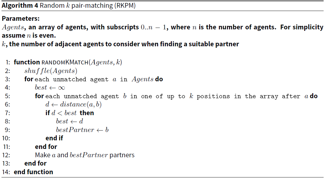
Surprisingly, unlike RPM the effectiveness of this simple algorithm is quite good in our applications. In effect assuming n agents in the matting pool, the algorithm randomly draws k elements without replacement from an ordered list of n elements, and selects l, the lowest of the k elements in the ordering. The mean position of l is \(\frac{1}{k + 1} \times n\) in the ordered list, and the median is \(1-e^{-\frac{\ln(2)}{k}} \times n\)
This means, for example, if we have k >= 100, then on average the partner chosen will be ranked in the top one percent in suitability from the remaining available agents.
Weighted shuffle pair-matching (WSPM)
This algorithm is an extension of RKPM, except that instead of ordering the agents entirely randomly, those with compatible pair-matching attributes are more likely to be clustered together. The algorithm works as follows:
Agents are assigned a cluster value. Then the cluster value is multiplied by a uniform random number — giving a random value weighted towards the cluster of the agent — to introduce stochasticism into the algorithm. Then the agents are sorted on this weighted value. Finally for each agent a, the agent with the smallest distance to a in the k adjacent agents is selected.
To calculate the cluster value for each agent, we need a domain-specific clustering function. This would typically be based solely on the attractor attributes, or a subset thereof, of the distance function. Despite being domain specific, a programmer without knowledge of the application can work out a cluster function solely by examining the distance function. However, it is likely that with greater domain knowledge, a more sophisticated cluster function can be defined.
Algorithm 5 is an example of a simple cluster function using some of the attractor attributes described above.
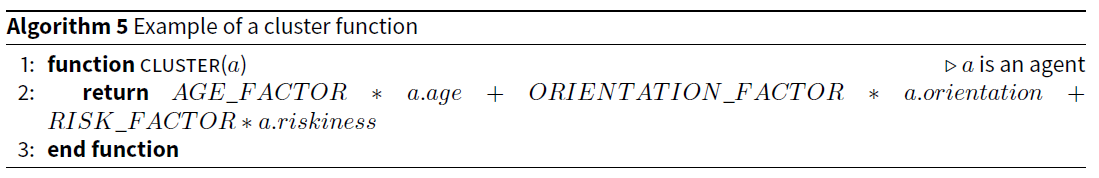
Algorithm 6 provides pseudocode for WSPM.
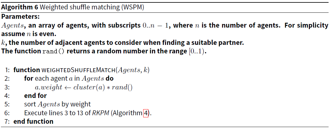
Assuming k is a constant, which it is in our implementation, then sorting has the slowest efficiency of the steps in this algorithm, linearithmic with the number of agents being matched. Therefore the efficiency of the entire algorithm is linearithmic with the number of agents.
Cluster shuffle pair-matching (CSPM)
This algorithm is a conceptual advance on WSPM. As with WSPM, it also extends RKPM and uses a cluster function. It works as follows:
The agents are sorted by the value returned by the cluster function (as opposed to a cluster weighted random number as in WSPM). They are then divided into a user-specified number of clusters. Then each cluster is shuffled to introduce stochasticism. (In contrast to WSPM, agents in the same cluster always remain relatively close to each other.) Finally, just as with WSPM and RKPM, it finds the best of k agents after the agent under consideration.
Algorithm 7 provides the pseudocode for this algorithm.

As with WSPM, the efficiency of the entire algorithm is linearithmic with the number of agents, because the only step that is not linear is the sort, which is linearithmic.
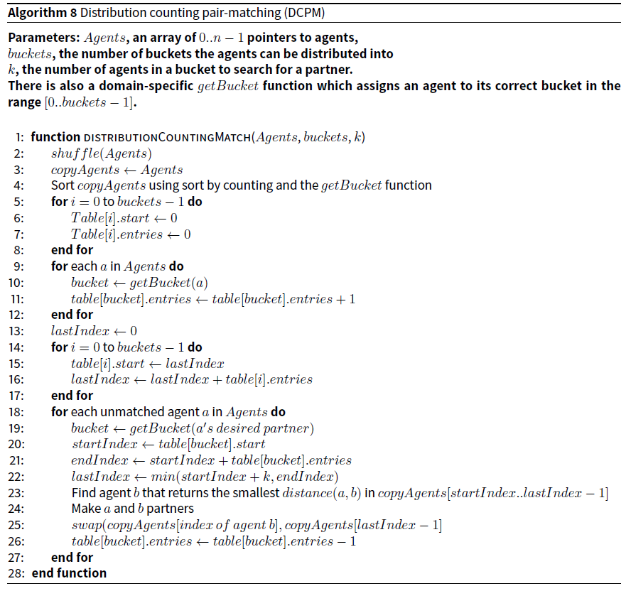
Distribution counting pair-matching (DCPM)
This algorithm is influenced by sorting by counting (Knuth 1998, p 75-79), also called distribution counting sort (Levitin 2011, p 283). It is only useful if the agents can be distributed into buckets that exactly or approximately correspond to the properties of the partners with whom they need to be matched. Therefore a domain specific function that places a given agent into one of a set of predefined buckets must be defined.
The algorithm works as follows: Pointers to the shuffled agents are copied into an array. The copy is sorted using distribution counting which makes use of the bucket function (Levitin 2011, p 283). This sorting has linear efficiency — as opposed to the linearithmic efficiency of standard sorting algorithms — because it uses information about the underlying distribution of the objects provided by the bucket function.
A table with the same number of entries as there are buckets is then constructed so that given the “desired” partner properties of an agent, a, we can directly access the first agent with those characteristics in the copied agents array. We then linearly examine up to k agents, selecting the partner with the closest distance. The algorithm uses a defined getBucket function which assigns an agent, or its “desired” partner to a bucket.
To understand how agents are assigned to buckets consider the agent properties of age, sex, and sexual orientation. If an agent representing a female “desires” a 25-year-old male, then it is assigned to the bucket of agents looking for 25-year-old heterosexual males. When looking for a partner, it will search up to k agents in this bucket and choose the one with the lowest distance to it. If the model’s agents are either male or female, heterosexual or homosexual, and any age from 16 to 50, then there are 2 * 2 * 35 = 140 buckets.
One caveat: Because age is a flexible characteristic (e.g. if the desired partner of a is 25 it does not mean that if b is a 24-year-old, it should have no prospect of partnership with a), the algorithm can be adapted so that it searches for a partner in several adjacent buckets, which differ by one or more years of age.
Assuming k is a constant, which it is in our implementation, the algorithm’s execution time is linear with the number of agents being matched.
The pseudocode for the unadapted algorithm is provided in Algorithm 8.
Methods
Simulation experiments
General set-up
To test and analyze the algorithms, two different simulations have been programmed that use the structure depicted by Algorithm 1. The two models differ in the properties of the agents and the distance functions. While the first (ATTRACTREJECT) is somewhat abstract and intended to explore the relative effect of attractor and rejector attributes, the second (STIMOD) resembles a more concrete application in the field of epidemiology taken from research on the HIV-epidemic in South Africa (Eaton et al. 2012; Hontelez et al. 2013; Johnson & Geffen 2016).
The purpose of these simulations is solely to test and compare the algorithms; the simulations are not intended to model the natural world. They also differ from simulations of the natural world in that every agent on every iteration (or time step) is in the mating pool, so that comparisons of the algorithms remain as fair as possible.
Both experiments were coded in C++ (ISO C++11) and compiled with the GNU C++ compiler version 4.8.4. Processing of results was conducted using R. The experiments were executed on a machine with an Intel Xeon with 20 cores running at 2.3 GHZ and with 32GB RAM, under the GNU/Linux operating system. The source code is available on Github at https://github.com/nathangeffen/pairmatchingalgorithms.
ATTRACTREJECT experiment
In the first microsimulation, which we call ATTRACTREJECT, every agent has two properties: attractor and rejector. When executing the simulation, the user sets two constants, ATTRACTOR_FACTOR and REJECTOR_FACTOR, to values between 0 and 1, such that they add to 1. The distance function is simple and the pseudocode for it is provided in Algorithm 9.
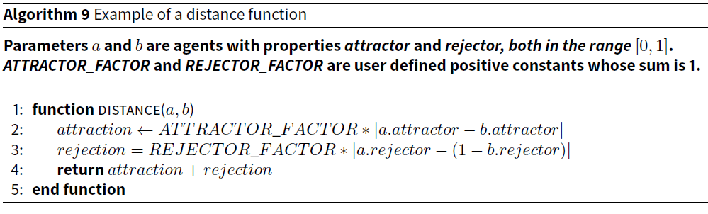
This distance function captures the issue of attractors and rejectors that affect the difficulty of the pair-matching problem when the triangle inequality is violated. The closer to 1 ATTRACTOR_FACTOR is set and the closer to 0 REJECTOR_FACTOR is set, the more clustered agents suitable for pairing will be. Conversely, the closer to 0 ATTRACTOR_FACTOR, the less useful clustering is, because agents that are clustered together will not be suitable matches.
STIMOD experiment
The ATTRACTREJECT model is not intuitive. The model in the second microsimulation (STIMOD), is intended to be more so. It is loosely based on previously published microsimulations (Johnson & Geffen 2016; Hontelez et al. 2013 ) that model the South African HIV epidemic, but much simpler than these. The pair matching characteristics of the agents are typical for a model of STIs: a list of previous partners, age, sex, sexual orientation and a variable that represents at how much risk of infection their sexual behaviour places them. We have also included an additional attractor factor in the distance function: location, described by x and y co-ordinates on a Euclidean plane, representing how far agents live from one another. An overview of the characteristics of the starting population can be found in Table 1.
| Variable | Range | Amount that distance function increases by (higher scores are poorer matches) |
|---|---|---|
| Age | Uniformly distributed over the ages 15 to 25 | AGE_FACTOR x the difference in age |
| Sex | 50% male/50% female | If mismatch on sexual orientation, add ORIENTATION_FACTOR x difference in sexual orientation (which is always 1) |
| Sexual orientation | 5% of males are men who have sex with men, 90% of females are women who have sex with women | |
| Risk index | Uniformly distributed over [0-1] | RISK_FACTOR x the absolute difference between two agents |
| Location | Uniformly distributed over a Euclidean plane with co-ordinates (0-10,0-10) | 0.1 x the Euclidean distance (DISTANCE_FACTOR) |
We emphasise that the model and distance function used here are solely for comparing the algorithms. “Production” standard models of the natural world would need to be more complex.
As with the ATTRACTREJECT model there are user defined constants that specify the weighting of each of these factors in the final distance calculation. The pseudocode for this distant function is provided in Algorithm 10.
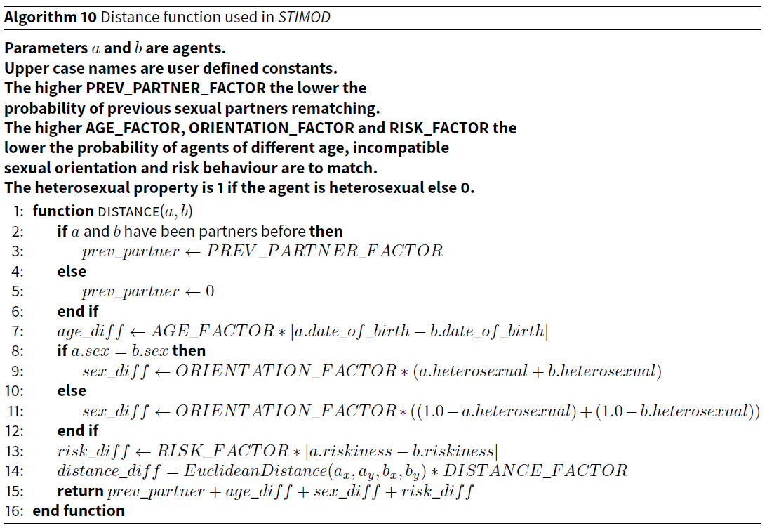
In all tests, we set PREV_PARTNER_FACTOR to 500, ORIENTATION_FACTOR to 100, AGE_FACTOR to 1, RISK_FACTOR to 1, and DISTANCE_FACTOR to 0.1 (see Table 2). Agents with similar ages, riskiness and location are more likely to partner, so these are attractors. Since 90% of agents are set to heterosexual, having the same sex is usually a rejector. Two agents who have been partners are also very likely to reject each other.
Measuring speed
To compare the speed of the algorithms, we ran 10 simulations of the STIMOD model for each algorithm using 20,000 agents. Each simulation was executed for 20 iterations (i.e. time steps). In other words every algorithm was executed 200 times.
We are also interested in how algorithms perform as the number of agents increases, or as the size of k increases for the algorithms that depend on this parameter. For the CSPM algorithm we are also interested in how the number of clusters affects speed. Since this algorithm achieved the best balance of effectiveness and speed in our tests, we ran tests on it varying the number of agents up to 10 million. We also ran tests varying k from 50 to 500, and tests varying c from 50 to 500.
Effectiveness and efficiency measures
Measuring effectiveness
We ran the following tests to compare the effectiveness of the algorithms in the STIMOD model:
- STIMOD with 5,000 agents, simulated 36 times with different random number seeds, with each simulation having 20 iterations. In other words, every algorithm executes 720 times. Algorithms were compared against Blossom V for effectiveness.
- STIMOD with 20,000 agents, simulated 36 times, with each simulation having 20 iterations.
- Using CSPM with 20,000 agents, we varied k, the number of adjacent agents to consider, from 50 to 1,000 stepping up by 50 on each execution of the microsimulation, while holding the number of clusters constant, to see the effect on the mean ranking and distance. We then similarly varied the number of clusters, c, initially setting it to 1 and then from 50 to 1,000 stepping up by 50 on each execution of the microsimulation, while holding k constant at 200.
We ran the following tests to compare the effectiveness of the algorithms in the ATTRACTREJECT model:
- ATTRACTREJECT microsimulation with 5,000 agents, with each simulation executed 20 times with different random seeds with the following combinations of ATTRACTOR_FACTOR and REJECTOR_FACTOR respectively:
- 0.0 and 1.0
- 0.25 and 0.75
- 0.5 and 0.5
- 0.75 and 0.25
- 1.0 and 0.0
- ATTRACTREJECT microsimulation with 20,000 agents, with each simulation executed 20 times with the above combinations of ATTRACTOR_FACTOR and REJECTOR_FACTOR respectively.
Best-possible result
As mentioned above, the mean distance and mean ranking measures can only be used for the relative comparison of the different algorithms. Furthermore, the set of partnerships with the minimum distance possible is not known a priori. This can be calculated using the Blossom V algorithm. A prerequisite for the application of Blossom V is the creation of a fully connected undirected graph where the vertices represent the agents and the edges represent the distances between them, a process with a quadratic speed increase with the number of agents being matched. The Blossom V algorithm itself is not stochastic and is very slow, with speed approximately cubic with the number of agents being matched. It is therefore only used for reference purposes in the simulations of 5,000 agents.
Mean of mean distances
In the first measure we calculate mean distance of all the pairings for a single execution of the pairing algorithm. Since every algorithm is executed multiple times, we calculate the mean of these means. The measure of effectiveness for an algorithm is then the mean of its mean distances divided by the mean of the mean distances calculated by Blossom V.
However, when we use 20,000 agents Blossom V is too slow to use. On high-end consumer hardware (an Intel Xeon running 20 i7 cores) a single execution of Blossom V over 20,000 agents, including creating the graph, takes over 2 hours — and we have had to run hundreds of simulations. Instead, effectiveness of the algorithm with the lowest mean of mean distances (usually BFPM) is assigned the value of 1. The effectiveness of the remaining algorithms is the ratio of their mean of mean distances to this algorithm’s mean of mean distances.
Mean of mean rankings
In the second measure for every agent we calculate the distance to every other agent, creating a fully connected undirected graph. For each agent, a, we can then order every other agent by its suitability as a partner to a. The ranking of a pairing for a given agent is its partner’s place in this ordering. If an agent chooses its ideal partner the rank is 0. If it chooses the least desirable partner, the rank is n – 2, where n is the number of agents being matched. We can then calculate the mean ranking over all the agents being matched for a single execution of an algorithm. We compare the algorithms by calculating the mean of its mean rankings over many executions. The lower the mean of mean ranking the better the algorithm has done.
Effectiveness is calculated analogously to the way it is done for the mean of mean distances measurement. Likewise with 5,000 agents effectiveness is established with Blossom V (although Blossom V guarantees lowest mean distance and not lowest mean ranking, in practice it generally returns the lowest ranking). With 20,000 agents, the method of assigning 1 to the effectiveness of the best algorithm is used.
Results
Speed tests
Table 2a lists the results of the speed tests. The fastest algorithm, RPM, has an average speed more than 5,700 times faster than the slowest algorithm, BFPM. The former completes the entire pair-matching event (i.e. match every agent for an iteration) in less than a millisecond on average, while the latter takes over three seconds on average. CSPM, RKPM, WSPM and DCPM have a mean speed between 27 and 39 milliseconds, and are all approximately an order of two magnitudes faster than BFPM.
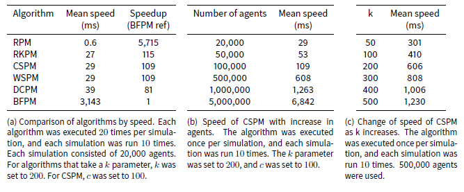 |
As the number of iterations increases, thereby creating more previous partners, the mean speed of the algorithms (except RPM) increases slightly, because the distance calculation has to search for more previous partners. For example BFPM increased from a mean of over 2 seconds on the first iteration of a simulation to 4.6 seconds on the 20th, and CSPM increased from 19 to 43 milliseconds.
The speed of the CSPM algorithm increased linearly with the number of agents, as Table 2b indicates. This is expected because even though our analysis above shows that its speed increases linearithmically with the number of agents being matched, this is due to its sorting operation, which is a small contributor to the overall time of the algorithm with these small numbers of agents.
Modifying the number of clusters also shows a linear effect on the speed of the algorithm. This is expected because modifying the value of c in Algorithm 7 increases the number of iterations of the for loop at line 8 although it correspondingly decreases the number of agents to be shuffled at line 11.
The speed of the CSPM algorithm also increased linearly with the size of k, as Table 2c indicates. This too is expected as increasing k proportionately increases the number of comparisons made for each agent a with the following agents in the array.
Effectiveness tests
Table 3 shows the results of the comparison of the algorithms on the STIMOD microsimulation for 5,000 agents. With this few agents, it is still feasible to identify the theoretically lowest mean distance using the Blossom V algorithm. In these tests CSPM, followed by DCPM algorithm, offers the best trade-off of speed and effectiveness. Nevertheless RKPM and WSPM have similar effectiveness and speeds.
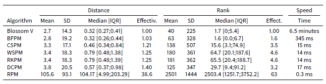 |
Table 4 shows the distance and ranking results respectively of the ATTRACTREJECT microsimulation. In contrast to the STIMOD microsimulation the DCPM algorithm is entirely unsuited to this distance function and performs poorly, although much better than RPM. The remaining algorithms improve their relative effectiveness as ATTRACTOR_FACTOR rises to 1 and REJECTOR_FACTOR declines to 0.
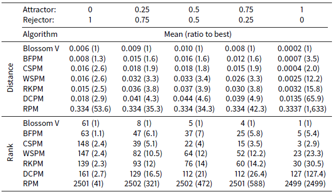 |
Interestingly CSPM exceeds the effectiveness of BFPM for higher values of ATTRACTOR_FACTOR. A possible explanation for this is that agents at the front of the array processed by BFPM will be well-matched, but agents nearer the back of the array have fewer partner options that give low distance measurements. CSPM, on the other hand, by first clustering, ensures the agents at the back of the array are nearer likely partners.
This raises a key weakness of BFPM, CSPM, WSPM, RKPM and possibly even DCPM: the distribution of their matches varies greatly in quality between the front and back of their arrays, and there is room for further research as to how they can be adapted to have a more equal distribution of quality.
Consider Table 6 which shows the mean median ranking, mean interquartile range (IQR) and mean standard deviation across the ATTRACTREJECT simulations with ATTRACTOR_FACTOR set to 0.5. The median ranking for BFPM is much lower than the mean ranking shown in Table 4. It is even better than the median ranking of Blossom V. In fact at least 75% of the rankings are better than the mean ranking, implying that some very poor rankings toward the back of the agent array bring down the mean ranking. This skewed quality is also a problem for CSPM but, as shown by its smaller standard deviation and median ranking closer to its mean ranking, not as profoundly as it is for BFPM, WSPM, RKPM and DCPM (see also Figure 2).
 |
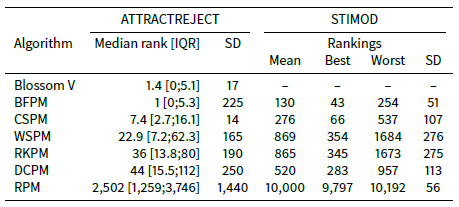 |

Table 4 also shows that when REJECTOR_FACTOR is much larger than ATTRACTOR_FACTOR, then as expected RKPM is as effective as CSPM, DCPM and WSPM.
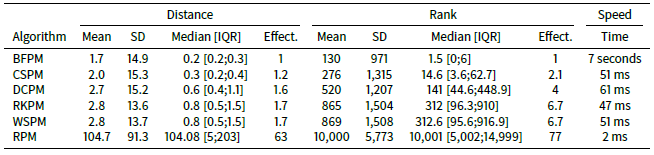
When the number of agents in the STIMOD model is increased to 20,000 (see Table 5) we do not see any substantial changes in effectiveness across the algorithms compared to when 5,000 agents are used, except that CSPM clearly outperforms DCPM on both mean distance and mean ranking. Whether this is due to something qualitatively different happening as the number of agents increases or due to random fluctuations of the results is unclear. The results from simulation to simulation are indeed volatile as Table 6 shows, with BFPM being the most stable algorithm followed by CSPM.
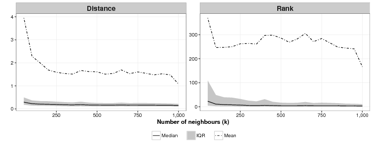
We also attempted to find the ideal values of k, the number of neighbours, and c, the number of clusters for the CSPM algorithm. As Fig. 3 shows, the relationship between the value of k and effectiveness is unclear for this application. For k = 50, the lowest value of k we tried, the mean of the mean rankings over 40 simulations was 370. For k = 1,000, the highest value of k we used, the mean ranking was 167, the lowest, but as the graph shows for all values in between, there is no discernible pattern. On other test runs we got different results where k = 1000 was not the best and k = 50 was not the worst. Results are domain dependent, and modellers who use CSPM will have to experiment to find the best value of k.
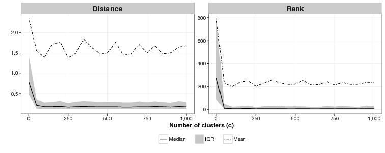
We are unsure what the relationship between c and effectiveness is as Figure 4 shows. For c = 1 (essentially an array sorted on the cluster function), the mean of the mean rankings is poor: 791. For all values of c tested from 50 to 1,000 we were unable to identify a discernible difference in effectiveness across the simulations. As with the ideal value of k modellers who use CSPM will have to experiment to find the best value of c.
Discussion
We have used two microsimulations to show how four algorithms CSPM, DCPM, WSPM and RKPM can match agents much better than chance (RPM) yet much faster than the BFPM algorithm and Blossom V — which finds a perfect set of pairs without desired stochasticism.
CSPM performed consistently well across our tests. For example in the STIMOD microsimulation it only had a mean ranking four times worse than Blossom V, whereas random matching was more than 61 times worse. When the number of agents was increased to 20,000, a number beyond which it is practical, at least on our hardware, to check effectiveness against Blossom V, CSPM’s mean ranking was only half as poor as that of BFPM, more than double that of the next best algorithm DCPM and 45 times better than random matching. Yet it executed on average in just over 50 milliseconds versus 7 seconds for BFPM.
However, while CSPM has done well here, it is likely that there are other applications where the other fast approximation algorithms, DCPM, WSPM and RKPM, will be equally good or better choices. We are currently exploring an application where DCPM appears to be better. In this application, the agents fall neatly into a pre-specified set of buckets, which is ideal for DCPM.
As the tests with the ATTRACTREJECT microsimulation show, when rejector attributes of agents dominate, the RKPM algorithm might as well be used: it is faster than CSPM, trivial to implement and will produce results that are at least as good as CSPM because clustering achieves nothing in such pair-matching scenarios.
CSPM requires the user to decide the values of two parameters, k and c. We cannot currently offer good heuristics for choosing these values other than to suggest preliminary empirical tests for the specific microsimulation being used.
We have not yet found a situation where WSPM outperforms all of CSPM, DCPM and RKPM. It is possible that it is simply an inferior algorithm, but it is not inconceivable that a useful microsimulation application exists in which WSPM makes sense as the pair-matching algorithm.
One serious limitation of BFPM, CSPM, RKPM and WSPM, at least in the applications considered here, is that the quality of their matches are skewed to the front of the array of agents that they process. After shuffling, agents near the front of the array will tend to be matched with partners with smaller distances than the agents at the back of the array. This is reflected in the fact that the mean of the median rankings — and even the 75% quartile — is smaller than the mean of the mean rankings in the simulations where we examined this. Further research is required to improve one or more of CSPM, RKPM or WSPM to reduce this skewed matching.
While we are interested in microsimulations that simulate sexual pairing, it is possible there are uses of these algorithms in other microsimulations which require agent interaction. However, for such applications the algorithms would need to be evaluated to see if they produce results that compare well to observed data.
Further research is also needed to see how useful an algorithm such as CSPM is in the context of modelling sexually transmitted infections. For example, the most cited model of the South African HIV epidemic is a deterministic equation-based one that implicitly assumes people are randomly matched (Granich et al. 2009). Other deterministic models of the epidemic make more complex assumptions, e.g. by dividing the population into a small number of sexual groups (Johnson 2014). It would be interesting to compare the outputs of a full-fledged microsimulation of an STI epidemic using random matching versus CSPM. If the results of such a microsimulation are similar irrespective of the pair-matching algorithm then the speed of random matching means it is the better choice. If however, the results are vastly different, it has implications for how we model, not only using agents, but also with deterministic differential-equation models.
References
ARYA, S., Mount, D. M., Netanyahu, N. S., Silverman, R. & Wu, A. Y. (1998). An optimal algorithm for approximate nearest neighbor searching fixed dimensions. Journal of the ACM, 45(6), 891–923. [doi:10.1145/293347.293348]
BEIS, J. S. & Lowe, D. G. (1997). Shape indexing using approximate nearest-neighbour search in high-dimensional spaces. CVPR '97 Proceedings of the 1997 Conference on Computer Vision and Pattern Recognition (CVPR '97). [doi:10.1109/CVPR.1997.609451]
BOUFFARD, N., Easther, R., Johnson, T., Morrison, R. J. & Vink, J. (2001). Matchmaker, matchmaker, make me a match. Brazilian Electronic Journal of Economics, 4(2).
COOK, W. & Rohe, A. (1999). Computing Minimum-Weight Perfect Matchings. INFORMS Journal on Computing,11(2), 138–148. [doi:10.1287/ijoc.11.2.138]
DEISSENBERG, C., van der Hoog, S. & Dawid, H. (2008). EURACE: A massively parallel agent-based model of the European economy. Applied Mathematics and Computation, 204(2), 541–552. [doi:10.1016/j.amc.2008.05.116]
EATON, J. W., Johnson, L. F., Salomon, J. A., Bärnighausen, T., Bendavid, E., Bershteyn, A., Bloom, D. E., Cam-biano, V., Fraser, C., Hontelez, J. A. C., Humair, S., Klein, D. J., Long, E. F., Phillips, A. N., Pretorius, C., Stover, J., Wenger, E. A., Williams, B. G. & Hallett, T. B. (2012). HIV treatment as prevention: systematic comparison of mathematical models of the potential impact of antiretroviral therapy on HIV incidence in South Africa. PLoS medicine, 9(7), e1001245. [doi:10.1371/journal.pmed.1001245]
GRANICH, R. M., Gilks, C. F., Dye, C., De Cock, K. M. & Williams, B. G. (2009). Universal voluntary HIV testing with immediate antiretroviral therapy as a strategy for elimination of HIV transmission: A mathematical model. The Lancet 373(9657), 48–57. [doi:10.1016/S0140-6736(08)61697-9]
GRAS, R., Devaurs, D., Wozniak, A. & Aspinall, A. (2009). An individual-based evolving predator-prey ecosystem simulation using a fuzzy cognitive map as the behavior model. Artificial Life, 15(4), 423–463. [doi:10.1162/artl.2009.Gras.012]
GRAY, R. T., Hoare, A., McCann, P. D., Bradley, J., Down, I., Donovan, B., Prestage, G. & Wilson, D. P. (2011). Will changes in gay men’s sexual behavior reduce syphilis rates? Sexually transmitted diseases, 38(12), 1151–1158. [doi:10.1097/OLQ.0b013e318238b85d]
HONTELEZ, J. A. C., Lurie, M. N., Bärnighausen, T., Bakker, R., Baltussen, R., Tanser, F., Hallett, T. B., Newell, M. L. de Vlas, S. J. (2013). Elimination of HIV in South Africa through expanded access to antiretroviral therapy: A model comparison study. PLoS medicine,10(10), e1001534. [doi:10.1371/journal.pmed.1001534]
INDYK, P. & Motwani, R. (1998). Approximate nearest neighbors: Towards removing the curse of dimensionality. In Proceedings of the Thirtieth Annual ACM Symposium on Theory of Computing, STOC ’98, (pp. 604–613). New York, NY, USA: ACM. [doi:10.1145/276698.276876]
JOHNSON, L. (2014). THEMBISA version 1.0: A model for evaluating the impact of HIV/AIDS in South Africa. Centre for Infectious Disease Epidemiology and Research, Working paper.
JOHNSON, L. F. & Geffen, N. (2016). A Comparison of Two Mathematical Modeling Frameworks for Evaluating Sexually Transmitted Infection Epidemiology. Sexually Transmitted Diseases, 43(3), 139–146. [doi:10.1097/OLQ.0000000000000412]
KNUTH, D. E. (1997). The Art of Computer Programming, Volume 2: (2nd Ed.) Seminumerical Algorithms. Redwood City, CA, USA: Addison Wesley Longman Publishing Co., Inc.
KNUTH, D. E. (1998). The Art of Computer Programming, Volume 3: (2nd Ed.) Sorting and Searching. Redwood City, CA, USA: Addison Wesley Longman Publishing Co., Inc.
KOLMOGOROV, V. (2009). Blossom V: A new implementation of a minimum cost perfect matching algorithm. Mathematical Programming Computation, 1(1), 43–67. [doi:10.1007/s12532-009-0002-8]
LAROSE, D. T. & Larose, C. D. (2014). k-Nearest Neighbor Algorithm, (pp. 149–164). John Wiley & Sons, Inc. [doi:10.1002/9781118874059.ch7]
LEVITIN, A. (2011). Introduction to the Design and Analysis of Algorithms. Boston: Pearson, 3rd edition.
MACY, M. W., & Willer, R. (2002). From factors to factors: Computational sociology and agent-based modeling. Annual Review of Sociology, 28(1), 143–166. [doi:10.1146/annurev.soc.28.110601.141117]
PELILLO, M. (2014). Alhazen and the nearest neighbor rule. Pattern Recognition Letters, 38, 34 – 37. [doi:10.1016/j.patrec.2013.10.022]
SCHOLZ, S., Surmann, B., Elkenkamp, S., Batram, M. & Greiner, W. (2016). Creating populations with partnerships for large-scale agent-based models - a comparison of methods. In Proceedings of the Summer Computer Simulation Conference (SCSC 2016), Simulation Series, (pp. 351–356). Red Hook, NY, USA: Curran Associates,Inc.
WEISSTEIN, E. W. (2016). Metric space. From MathWorld – A Wolfram Web Resource: http://mathworld.wolfram.com/MetricSpace.html.Accessed: 16 November 2016.
ZINN, S. (2012). A Mate-Matching Algorithm for Continuous-Time Microsimulation Models. International Journal of Microsimulation, 5(1), 31–51.