
Introduction
The networks of interacting entities have been of great interest in complex system analysis, since complex systems demonstrate emergent behavior that cannot be trivially predicted. Network dynamics in self-organized systems is determined by agents’ behavior, whereas the states of the agents often depend on local topological characteristics. This co-evolution of the states of nodes and the network usually demonstrates unpredictable behavior due to the presence of cascades of feedback links, which are difficult to observe. In this way, along with the evolution law, the network topology significantly affects the resulting stability of a system.
Interconnections between the network topology and domain properties of a system were studied from static (Dörfler et al. 2013; Roukny et al. 2013) and dynamic perspectives (Ahnert & Fink 2016; Liu et al. 2014). The static perspective (when the network structure does not evolve over time) usually considers changes in the node states because of a dynamic process spreading on a fixed topology (Tambayong 2009). The result of process spreading may be estimated as positive or negative (e. g., spreading or absorbing some shock). In this way, tipping points in the system parameters may be discovered (Dorogovtsev et al. 2008). Numerous economic studies on the topology of interbank networks emphasize its role in times of crisis (Gupta et al. 2013; Haldane et al. 2009; Lux 2016; Steinbacher et al. 2016). Additionally, the values of network structural invariants are related to successful outcomes of financial shock (Gai et al. 2011; Nier et al. 2007). The empirical data confirm the distinction between pre- and post-crisis networks (Boss et al. 2004; Iori et al. 2008; Soramäki et al. 2007).
Dynamical statement captures an additional level of complexity by considering the changes in the network structure (i.e. temporal networks[1]) along with the changes in node states. The capacity of a system to adapt to environmental changes, the rapidity of responses, and the resulting complexity of a system have led researchers to consider temporal networks as “black boxes” (Bernanke & Gertler 1995). Therefore, we explore the network formation dynamics to find a method to make the system more resistant to shock contagion in times of crisis. In other words, we determine how the entities in a banking system should interact to form a network that remains stable over time (e.g., to determine which constraints should be applied for bank portfolios to increase the overall network stability). Understanding of these processes allows for making a system more resistant to shock, which is important since banking crises have been shown to be highly correlated with economic crises (Goodhart et al. 2004; Larionova & Varlamova 2014).
A temporal network undergoes significant changes during its evolution because of edge formation, rewiring, and deletion, and it changes in the number of nodes. These topological changes may be related to more than one driver in the system. The mechanisms of partner choice—the algorithms for choosing pairs of nodes (bank-bank or bank-customer) to create an edge between them—have an important role in the formation of the topology of an interbank network. Lenzu & Tedeschi (2012a) introduced a measure of agent attractiveness, which allows to generate different network topologies while varying the parameters of counter-party choice policy. Halaj & Kok (2015) modeled new interbank link formation as a bargaining game, and Iori et al. (2015) used the choice model with memory. Topological dynamics is also affected by market clearing models (Aldasoro et al. 2015) that are applied when a bank is eliminated from the network; nevertheless, the aforementioned research was focused on one driving force of network dynamics, the optimization of agent portfolios.
There are studies considering several driving forces of evolution of interbank networks (namely, behavioral rules of banks and customers) and the influence of these drivers on the systemic stability (Arslan et al. 2016; Delli Gatti et al. 2010; Robertson 2003). However, these works usually focus on the result of simulations without studying how the topology changes during simulation or how different behavioral rules interact, spawning non-linear effects. A layer of macroeconomic agent-based models (Grilli et al. 2015; Delli Gatti & Desiderio 2015) considers the combination of several components in a system (firms, customers, banks, trading models, profits and losses models, and monetary policies variations). These studies are examples of the exploration of a system property affected my several driving forces simultaneously and investigating emergent properties of a system. In contrast to our research, they study macroeconomic properties affected by the changes in, for example, monetary policy (Delli Gatti & Desiderio 2015), while we consider emergent effect on topological interbank network properties.
The evolution law of a banking system with several evolutionary drivers (this law describes the emergent behavior of a system owing to interactions of different entities per the predefined rules) seems to be too complex to be presented mathematically. In addition, making precise models may be inappropriate since “state-of-the-art is evolving over time” and models lose accuracy (Goodhart et al. 2004). The simulation solves several out-lined issues. Existing simulators allow for establishment of a set of rules for the behavior of agents and for the study of the evolution of a network (Schaul 2011; Quax et al. 2011). Nevertheless, they are either too general to analyze the multi-factor formation of an interbank network (which is the goal of the simulation tool pro-posed in this paper) or to be oriented to other domains. Some of the simulators only allow simple integer states of agents (Schaul 2011) and do not support real-valued states or representing a state by a vector of parameters. Other tools are oriented to the described systems with ordinary differential equations (Gorochowski et al. 2009). SEECN, in the frame of DynaNet project (Sloot & Erenstein 2009), aims for the efficient simulation of complex-network dynamics. It considers each edge and node state as a vector that is processed by a function determining the evolution of a system. Nevertheless, it focuses on general-network dynamics and is inappropriate for exploring multi-factor mechanisms of interbank-network formation. The overwhelming majority of simulation tools do not allow the exploration of temporal complex networks (Rahman et al. 2009).
To support the exploration of temporal networks on the different levels of granularity, corresponding simulation tools should have a modular structure allowing different representations of the main entities and functions of a system. The current study is intended to provide the tool oriented to the exploration of time-evolving interbank networks on the one hand, and, on the other hand, is sufficiently generic to solve different kinds of problems (in contrast to the existing algorithms in the field that are designed to answer research questions) on the other hand. To do this, we use general domain-specific simulation scheme which can further be supplemented with any necessary algorithms for different steps of the scheme. These steps (which are required to update states of nodes and the topology of a network) may be “overloaded” (in terms of object-oriented programing) in a variety of ways to study different aspects of the behavior of a system. Thus, competitive simulation tool for temporal networks focus on two goals: (i) to maintain the specificity of a domain area, and (ii) to provide sufficient flexibility, i.e., to support different models of network entities and algorithms of their interactions.
This paper is dedicated to the design and implementation of the simulation tool for temporal networks encountered in interbank relations. We incorporated several driving forces specific for the formation of interbank networks into the generic model while supporting different implementations of the domain-specific algorithms such as strategies of counter-party choice. As an example of the problem that requires the usage of simulation tools for temporal interbank networks, one can consider the problem of finding the optimal regulation constraints leading to the formation of stable network topology[2] under fixed conditions. The main difficulty in the problem is the absence of a general model able to determine how banks should choose counter-parties to obtain the preferable resulting topology. Therefore, a simulation tool with a set of tunable parameters, extensible banking network entity models, and different counter-party choice algorithms seems to be the most appropriate instrument to explore such kinds of problems.
The evolution of a dynamic network results from edge (or/and node) addition, deletion, and rewiring. In terms of a banking system, each network modification type corresponds to an activity in a banking system, prevailing in different times. Edge addition results from the creation of interbank exposures triggered by the changes in bank portfolios, while an edge is deleted after the loan term expires. Since both bank and customer activities affect portfolio dynamics (an increase/decrease in assets or liabilities), we consider at least two driving forces as the simplest case. For example, banks interacting with customers more have their portfolio modified more frequently, and therefore interact more intensively with other banks. In this way, partner choice for both customers and banks affects network-topology dynamics. Clearing algorithms, the algorithms of edge rewiring after bank defaults, and shock-contagion mechanisms also contribute to the topological dynamics. Additionally, the default-contagion mechanism, in terms of networks, is the deletion of a node corresponding to a default bank with the spread of residual shock among its neighbors. Depending on the shock size, contagion defaults can appear, which sometimes results in knock-on effects (which are also called domino-effects or avalanches). In addition, the removal of nodes (and consequently, the reduction in edge number) affects most of the network invariants to a large extent. To explore the impact of all these factors on the resulting topology, we propose a general scheme to simulate the evolution of temporal interbank networks and the example of implementing this scheme based on particular models of network entities and the algorithms of network dynamics. As the interbank network structure has been shown to be especially important in times of crisis (Gai et al. 2011; Georg 2013; Grilli et al. 2015), the proposed simulation tool incorporates different stability metrics and topological metrics. The analysis of the evolution of an interbank network is additionally supported by the visualization tool.
The rest of the paper is organized as follows. We present the general simulation scheme and the particular implementation of this, including the formalized description of modeling entities and algorithms of their interactions. As the proposed simulation tool has a modular structure, particular models and algorithms could be modified, extended, or supplemented to fit the reality in desirable extent and to provide a more comprehensive exploration per the goal of substantive studies. We further observe network topological invariants and stability metrics implemented in frames of the simulation tool to analyze the system structure and to evaluate evolutionary dynamics. The results of experiments for the artificial networks, while varying the counter-party choice algorithms and model parameters, and the results and conclusions on computational complexity and scalability of modeling algorithm are presented in the last section.
The Model Description
Generally, the model of a system is a set of its internal and external entities (represented by nodes) and the list of relations between them (edges). For temporal networks, edges can disappear if they have a restricted lifetime, and can be added (with some certain attributes) by network agents when the agents optimize their states. Interbank network agents in particular tend to maximize their profit and minimize loss, during asset allocation, and satisfy regulatory restrictions, on other hand. Their state is described by a set of optimized variables. This is an example of how self-organization occurs in temporal networks.
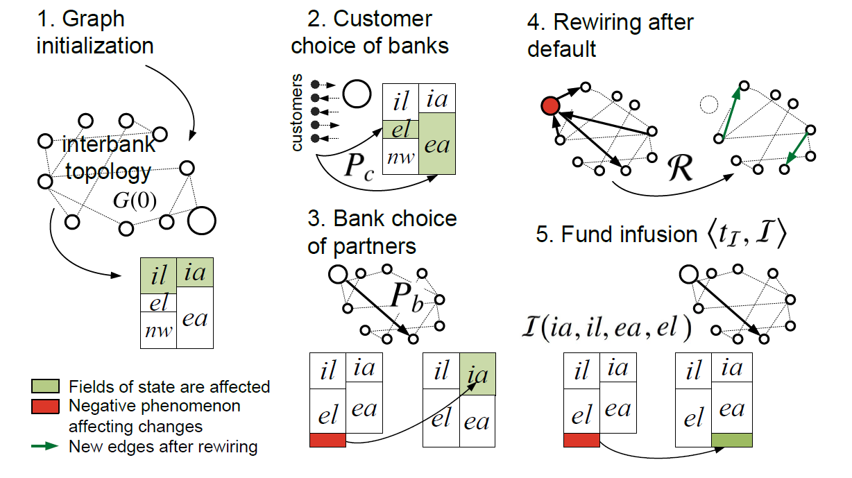
The current section describes the evolution model of a temporal network specialized for an interbank market. Summarizing the line of research on temporal interbank networks, we distinguish several common steps which could be performed during a single iteration of a simulation. Figure 1 shows five components of a general simulation scheme that affect the process of network formation. These components serve as a basis for the proposed simulation tool. First, the initial topology of an interbank network should be provided as an input for the tool (step 1 in Figure 1). The topology can be created by the simulator (using existing network generative models) or provided by a user (for cases where real data are available). Also, the step of initialization includes the assignment of node states based on current network structure (see Figure 1, where a bank state is represented by its balance sheet). Step 2 creates edges between customers and banks; therefore, it is executed when the model includes customer-nodes which can borrow or lend from/to a bank. The number of customers for each iteration is supposed to be known. Each customer chooses a bank per the predefined partner-choice algorithm. Step 2 results in bank balance sheets being updated. Step 3 illustrates the similar step of partner choice for banks, which triggers interbank network formation per the predefined algorithm. Step 4 presents how edge redistribution is performed in the network after a node elimination. Step 5 (fund infusion) represents the external influence on the system, which modifies node states and network topology in some evolution periods. As an example of such effect, we present a central bank fund infusion aimed at stabilizing bank states if necessary. Generally, some other external factor or implementation of a central bank could be used instead.
In this study, we present the implementation of the scheme, which generalizes the scheme presented by Guleva et al. (2016) and brings together several different models which contribute to the evolution of an interbank network. The detailed description of state parameters (parts of the models of a bank and a customer) and the algorithms used in the implementation are presented further in the current section.
Each iteration of the simulation may result in different topologies and different states of nodes. Therefore, the system description is followed by a detailed description of metrics used for quantitatively estimating the changes.
The network model
Typical interbank network models (Allen & Gale 2000; Gai & Kapadia 2010; Steinbacher et al. 2016) take banks as nodes and interbank lending as edges on a graph. This representation may be described as a graph (Gai et al. 2011; Georg 2013) or as the corresponding liability adjacency matrix (Boss et al. 2004; Upper 2011). Since the influence of both banks and customers is considered in our work, we suggest expanding the conventional interbank market model with two types of nodes and two corresponding subnetworks. Therefore, a banking network contains a set of banks, a set of customers, list of edges in the interbank network, and list of edges in the external network (consisting of the edges between banks and customers). Edges are directed and attributed with weights and maturities. The weight is the amount of money involved in the interaction represented by an edge. The amount of money can be a fixed constant or can be chosen randomly, and the maturity, which represents lifetime of an edge, can also be random. Namely, it presents how many iterations are performed before the edge disappears. Since lending is distinguished between different kinds of terms (Cox et al. 1985), we first choose the term group randomly, and then the final term of liability within the group is chosen. This may be varied depending on the banking system explored, because the maturity structure may differ (Kim & Singleton 2012; Smaga et al. 2016).
Output links correspond to bank assets, and input links correspond to liabilities, as in (Upper 2011) where adjacent matrix rows correspond to assets. In addition, each pair of banks can be connected with more than one edge regarding different attribute values.
Therefore, the banking system is a dynamic directed multigraph with weights and maturities of edges:
| $$G(t)=(\mathbf{B}(t),~\mathbf{C}(t),~ E_{ib}(t),~ E_{ext}(t))$$ | (1) |
| $$E_{ib}(t) = \{e=(i,j,w,m)~ |~ i, j\in \mathbf{B}(t),~ w\in \mathbb{R}^+,~ m\in \mathbb{N}\}$$ | (2) |
| $$E_{ext}(t) = \{e=(i,j,w,m) ~|~ i\in\mathbf{B}(t)~ \wedge~ j\in\mathbf{C}(t)~ \vee$$ |
| $$\vee~j\in\mathbf{B}(t)~ \wedge~ i\in\mathbf{C}(t),~ w\in \mathbb{R}^+,~ m\in \mathbb{N} \},$$ | (3) |
The bank model
The bank model is presented by its balance sheet, which consists of interbank and external assets and liabilities and net worth, which is the difference between the assets and liabilities. This structure allows for designing the default condition and the interrelation between external effects on bank balances and interbank activity, which is necessary to avoid defaults. In addition, interbank interactions are well-defined in terms of network science, which is widely used in other studies (Gai & Kapadia 2010; Haldane & May 2011; Nier et al. 2007; Upper 2011) in more or less detailed variations. External assets and liabilities of a bank are formed by the output and input links from the external network, and interbank interactions are formed by the edges from the interbank network:
| $$ia(i,t)=\sum_{(i,j,w, m)\in E_{ib}(t)}{w},$$ | (4) |
| $$il(i,t)=\sum_{(j, i,w, m)\in E_{ib}(t)}{w},$$ | (5) |
| $$ea(i,t)=\sum_{(i,j,w, m)\in E_{ext}(t)}{w},$$ | (6) |
| $$el(i,t)=\sum_{(j,i,w, m)\in E_{ext}(t)}{w},$$ | (7) |
| $$nw(i,t)=ea(i,t)+ia(i,t)-el(i,t)-il(i,t).$$ | (8) |
The net worth determines the state variable \(s_i\) of a bank in this model. The satisfactory lower bound of the state variable is \(s_0\). If \(s_i<s_0\), then the process of creation of new interbank links is triggered.
For the case of two variables characterizing the state of a bank, the balance sheet is extended with cash and operating cost parameters to demonstrate the dualism of bank optimizing policy. The model of the balance sheet with cash variable can be seen in (Krause & Giansante 2012). While net worth \((nw\)) tends to increase with a growth of asset size and decrease with a growth of liability size, cash \((cash)\) demonstrates opposite monotony. Each bank needs to balance between net worth and cash values to have those both non-negative[3]. An operating cost parameter \((oc\)) indicates the value deducted from the cash on each iteration.
| $$\begin{align*} \forall b\in\mathbf{B}:~ nw(b,t),~ cash(b,t),~ \Delta ia(b),~ \Delta ea(b),~ \Delta il(b),~ \Delta el(b) \Rightarrow \\ \Rightarrow nw(b,t+1)=nw(b,t)+ \Delta ia(b) + \Delta ea(b) - \Delta il(b) - \Delta el(b), \\ ~ cash(b,t+1)=cash(b,t) - oc(b) - \Delta ia(b) - \Delta ea(b) + \Delta il(b) + \Delta el(b), \end{align*}$$ |
The customer model
Existing customer models consider multiple factors of their decision making. These models describe the correlation between personal and other characteristics (Calem & Mester 1995) and are aimed at predicting consumers’ decisions (Capon et al. 1996). In our current research, we are interested in a much simpler model, where borrowing and lending and their size are distinguished. Since we have not met up analogous in the literature, we use the following naive implementation. The customers represent firms and organizations. Each customer has an account (referred to as a customer's state - \(s_c\), which corresponds to the total amount of money available. This amount determines the attributes of the edge created by a customer. If a customer's state is greater than \(\delta\), a threshold determining average necessary vital resources per customer, then an output link is produced; otherwise, an input link is produced. In this way, \(delta\) distinguishes customers who need resources and ones who have redundant resources. The weight of a new edge is proportional to the state value. Therefore,
| $$\forall c\in\mathbf{C}~\Big( s_c < \delta \Rightarrow e=\big(b, c, \frac{2\cdot\delta-s_c}{\zeta}, m\big)\Big) \wedge \Big( s_c \geqslant \delta \Rightarrow e=\big(c,b,\frac{s_c}{\zeta}, m\big) \Big),$$ |
The model of network evolution
A network evolution begins with an initial topology, which can be constructed by one of the following means: (a) according to complete empirical data, (b) reconstructed with empirical incomplete data of total interbank assets and liabilities and topological properties, or (c) constructed with graph generative models. Then, the network undergoes step-by-step changes after the actions of customers and banks. Each bank may request a central bank for infusion of funds once during the simulation to avoid going bankrupt; in addition, failed banks are eliminated from the network, triggering the rewiring of edges. The structure of an interbank network is directly affected by the counter-party choice algorithms. The weights and the maturities of edges influence the rapidity and the intensity of changes in the structure. The network structure may also be modified after bankruptcies, since this initiates the rewiring of edges. In the case of bankruptcies, the processes of shock absorption or contagion within a given network can be observed.
We describe the parameters determining the evolution of a temporal interbank network with the following septuple:
| $$\mathcal{E} = \bigg<G(0), P_b, P_c, \mathcal{W}, \mathcal{M}, \mathcal{R}, \big<t_{\mathcal{I}}, \mathcal{I} \big> \bigg>,$$ | (9) |
The counter-party choice algorithms
The counter-party choice policies represent a method for banks or customers to choose a counter-party (a bank) for interaction. The implementation of these policies provides the realization of steps 2-3 in Figure 1.
Let \(\mathbb{G}\) be the set of all possible networks, \(P_c\) be a customer choice policy, \(P_b\) be a bank choice policy, and \(P_a\) be a policy for any node type. Without loss of generality, the choice function \(P_a\) is defined as follows:
| $$P_a: [\mathbf{B}\cup\mathbf{C}]\times\mathbb{G} \rightarrow \mathbb{N} ~\big|~ \forall i\in \mathbf{B}\cup\mathbf{C}~ ~\forall G(t)\in \mathbb{G} ~~\forall w \in\mathbb{R}^+ ~~\forall m \in\mathbb{N} ~~~ \Big(i, P_a\big(i, G(t)\big), w, m\Big)\in E_{ib}(t+1)\cup E_{ext}(t+1)~~ \bigvee$$ |
| $$~~ \bigvee ~~ \Big(P_a\big(i, G(t)\big), i, w, m\Big)\in E_{ib}(t+1)\cup E_{ext}(t+1). $$ | (10) |
Despite customer choice being mostly affected by the image of the bank; the efficiency, quality, and speed of service; and interest rates (Siddique et al. 2012), we restrict ourselves to random and preferential models in this study, as they can form different types of topologies. In addition, the assortative method is also supported for the banks (banks with the high similarity measure values have greater probability to be connected).Therefore, we use random (R), preferential (P), and assortative (A) counter-party choice policies. Let \(p_c(i)\) and \(p_b(i)\) denote the probabilities that \(i^{th}\) bank will be chosen for interaction by a customer and a bank, respectively. If the policy can be used by both banks and customers, then \(\forall a\in\mathbf{B}\cup\mathbf{C}, ~\forall i\in\mathbf{B}\) we denote the probability as \(p_a(i)\).
Random choice policies of a bank or a customer imply equal probabilities to choose any of banks, that is:
| $$p_a(i)=\frac{1}{|\mathbf{B}|}. $$ | (11) |
Preferential choice policies imply that the probability of a bank to be chosen is proportional to the size of its asset. Therefore,
| $$\forall i\in\mathbf{B}~~ p_a(i)=\frac{ea(i)+ia(i)}{\sum_{b\in\mathbf{B}}{ea(b)+ia(b)}},$$ | (12) |
Assortative policies provide a higher clustering coefficient in comparison to other types of policies. When assortative policy is used, the closest bank to a given bank (in terms of the distance between their asset values) is chosen to create the connection. This is applied only for banks because the assortative rules imply the comparison of the structures of bank balance sheets. Therefore, the probability of bank \(b\) to choose bank \(i\) is
| $$p_b(i)=p~ \bigg(i=argmin_{j\in\mathbf{B}}{\big(\big|ia(j)+ea(j) - ia(b)-ea(b)\big|\big)\bigg)},$$ | (13) |
Edge rewiring algorithms: the elimination of a node
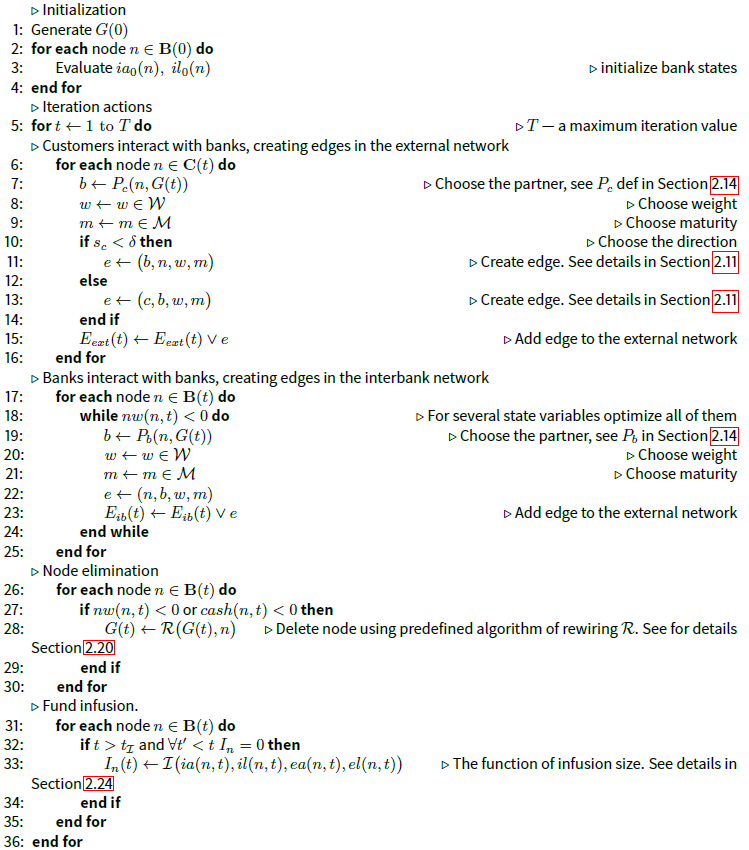
The algorithm of bank elimination (step 4 in Figure 1) significantly affects the network evolution in times of avalanches. We assume funds to be redistributed between counter-parties in a pre-established way (according to one of the algorithms). Firms and banks, both, are considered during this process. According to generalized algorithm description (Algorithm 2) all input and output edges adjacent to defaulted bank are sorted in corresponding lists and, after that, each pair of top edges from the lists is replaced with an edge connecting the borrower and lender of a bankrupt. All agents from the bottom of the list, without counter-party assigned, are supposed to lose their funds. The resulting topology after this procedure may vary, due to the weight and the maturity structure of edges linked to an eliminated bank. All the algorithms for edge rewiring implemented in this study are based on sorting input and output links of a bank, that went bankrupt. After the sorted links are rewired between other banks, the balance sheets are updated.
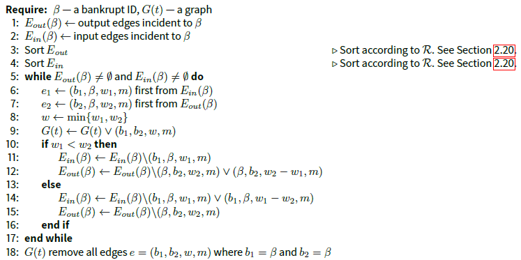
In this paper, we present the following sorting algorithms: (i) random (\(r\)), (ii) sorting per to lending repayment urgency (\(u\)), (iii) assortative and disassortative attachment (the algorithms and corresponding abbreviations are illustrated in Figure 2).
The first sorting method (i) keeps links in the order they were created. The second algorithm (ii) considers the maturity structure. It indicates the most urgent edges to be rewired first. In this way, the first banks from a liability list are linked to the first banks from the asset list. Therefore, assets and liabilities of a failed bank are sorted by their repayment dates. The third approach (iii) implies assortative and disassortative mixing. Edges are sorted by the asset size of the banks to which they are adjacent. Considering the link directions and both the straight and reverse orders of sorting, we obtain four possible mixing combinations:
- The banks with the largest assets go first in both input and output link lists (LL);
- The banks with the smallest assets go first in both input and output link lists (SS);
- In the liability list, the bank with the largest asset goes first, while in the asset list, the bank with the largest assets goes last (LS);
- The bank with the smallest assets goes first, and in the liability list, the smallest one goes last (SL).
In the simplest case, when a default is associated with the negativity of net worth in the model, assets are less than liabilities. Consequently, after rewiring there are some banks affected by a shock, which may potentially trigger a cascade of defaults. Therefore, an algorithm of rewiring Algorithm 2 affects possible losses.
Central bank infusion
The mathematical formalism presented in current subsection intends to describe possible external impacts on node states affecting topological dynamics. We consider central bank injections as an example of such influence. Despite central bank restrictions affecting banking system evolution and significantly controlling it, we attempt to distinguish factors driving single bank policies over all simulation and factors affecting network evolution in some certain periods, e.g. in times of crisis. Generally, this representation can be extended to more or less accurate central bank models or other external factors affecting network formation, or redefined.
The central bank infusions may prevent the triggering of node elimination, therefore complicating the evolution dynamics to some extent. If \(I(t)=\big(I_1(t), I_2(t),\dots, I_N(t)\big)\) is an infusion vector at the iteration \(t\), then, for all banks \(b\in\mathbf{B(t)}\), that means \(cash(b,t)=cash(b,t-1)+I_b(t),\) which allows the bank to increase the asset size in the near future.
Central bank infusion is a fund that may be injected to a bank at some moment during modeling. This is allowed once for each bank during simulation. We implement infusion depending on the iteration and size of infusion. The first parameter, an iteration of infusion \(t_\mathcal{I}\), means that infusion cannot occur before this moment. The second parameter is a function of infusion size, which takes the bank balance sheet values as input and returns the desired infusion size for the bank.
Let \(\big<t_{\mathcal{I}}, \mathcal{I} \big>\) be infusion parameters, where \(t_\mathcal{I}\) is an iteration of infusion, and the function determining the size of the desired infusion for some bank \(b\) is defined as \(\mathcal{I}:\mathbb{R}^4\rightarrow \mathbb{R}\). This takes as input the real number values of its balance sheet \(\big(ia(b,t), il(b,t), ea(b,t), el(b,t)\big)\) and returns the desirable infusion size for a bank.
Therefore, the infusion vector describing injections for all banks and all iterations can be defined as follows:
| $$I(t)=\big(I_1(t), I_2(t), \dots, I_N(t)\big),$$ | (14) |
| $$ I_j(t) =\left\{ \begin{array}{ll} \mathcal{I}\big(ia(j,t), il(j,t), ea(j,t), el(j,t)\big)\\ 0,~\forall j\in\mathbf{B},~t<t_\mathcal{I} \\ 0,~\exists t'<t:~ I_j(t_1)\neq 0 \end{array} \right.$$ | (15) |
Dynamics Evaluation: Metrics
The topological dynamics are measured with the network invariants - namely, the average degree, average clustering coefficient, and average shortest path. These invariants are chosen since they are mostly used in empirical networks analysis and therefore there is more information regarding the corresponding values of real world networks. During the calculation of average degree, we consider the presence of multi-edges in a graph, so the degree is calculated as the sum of the weights of edges adjacent to a node. Literature on empirical interbank networks show the average degree to be about 15-23 (Leonidov & Rumyantsev 2014; Cont et al. 2010; Roukny et al. 2013), the average clustering coefficient to be between 0.12 and 0.87 (Boss et al. 2004; Roukny et al. 2013; Soramäki et al. 2007), and the average path length to be near 2.26–2.6 with the diameter in 5–7 (Cont et al. 2010; Boss et al. 2004, Soramäki et al. 2007). Another topological metric, which is currently implemented in the simulation tool, the Entropy feature, was introduced by Ye et al. (2015). This is the entropy of graph Laplacian spectrum metric, and we used it since the Laplacian spectrum sufficiently reflects network structure, as it is sensible for the change in the number of edges, reflects number of leaves, maximum degree, algebraic connectivity, and other properties[4] (Merris 1998; Mohar et al. 1991). Applied to the network model of a banking system, it can be represented as follows:
| $$Entropy(t) = 1-\frac{1}{N} - - \frac{1}{N^2}\cdot \sum_{n_1, n_2\in \mathbf{B}}{\frac{1}{\big(ia_t(n_1)+il_t(n_1)\big)\cdot\big(ia_t(n_2)+il_t(n_2)\big)}}.$$ | (16) |
The qualitative state of the system can be estimated with the number of banks with negative net worth for the models without a mechanism of node elimination, and with the number of eliminated nodes for the models providing such a mechanism.
To evaluate the dynamics of node states and the overall stability of a system, we use the metrics of velocity and remoteness of nodes from an unsatisfactory state, and the \(\mathscr{T}\)-threatened set of nodes, which were introduced by (Guleva 2016a). An unsatisfactory (critical) state of a node is some value of a state variable, approaching to which indicates some additional dynamics, and, finally, the node elimination occurs. The definitions of velocity and remoteness are the following (Guleva 2016a):
Let \(N\) be a number of nodes, let \(S(t)=(s_1(t), ..., s_N(t))\) be a state of the network, where \(s_i(t)\) is a node state at iteration \(t\). Let \(s_0\) be the critical state of a node for some model.
Definition 1 Node velocity \(v_i\) at iteration \(t\) determines the change of a node state per iteration and is defined as
| $$v_i(t)=s_i(t)-s_i(t-1).$$ | (17) |
Definition 2 Node remoteness \(r_i\) at iteration \(t\) determines a number of iterations which is necessary for node of state \(s_i(t)\) having the velocity \(v_i(t)\) to reach the value of its critical state \(s_0\), and defined as
| $$r_i(t)=\frac{s_i(t)-s_0}{|v_i(t)|}$$ | (18) |
Using the definitions above, the authors introduced the function reflecting the relative number of nodes approaching their critical state:
Definition 3\(\mathscr{T}\)-Threatened set of nodes \(D_\mathscr{T}(S)\) for the network of state \(S\) contains nodes having negative velocity and remoteness, which is less than \(\mathscr{T}\).
$$D_\mathscr{T}(S)=\big\{ i|s_i>s_0, v_i<0, r_i<\mathscr{T} \big\}$$ (19)
This set is aimed at recognizing when most of the nodes have negative dynamics and when the knock-on effect can be induced with node-state dynamics more than with the network topology state. We consider the node-state oriented features to distinguish cases when the topology does not have a significant contribution to the cascades of defaults. This means that mass bankruptcies may be triggered mostly by the gradual deterioration of node states rather than topological influences.
The Experimental Study
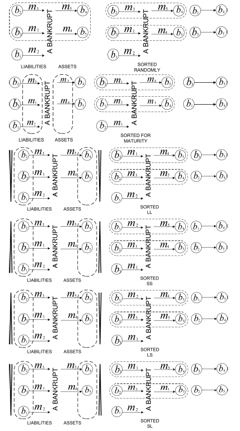
Following Castiglionesi & Eboli (2015), Cohen-Cole et al. (2015), Lux (2015), and Nier et al. (2007), we focused on reproducing driving forces and results of shock contagion for a simplified model rather than the nuanced investigation of evolution of real-world interbank network (such investigation is significantly hampered by the lack of necessary data, e.g. exact values of interbank liabilities and even the structure of a network itself). The model of temporal interbank networks presented above was used to implement the simulation tool supporting different realizations of steps 1-5 in the general simulation scheme (Figure 1). The simulator was implemented with C# programming language. The source code is published (Guleva 2016b) and available on-line (https://www.openabm.org/model/5285/version/1/view). Face validity, tracing, and internal validity methods were used for the model verification and validation (Xiang et al. 2005). Along with the general simulation algorithm, the current version of the simulation tool implements all particular algorithms introduced above, namely:
- Generative models for artificial networks (the generative models of all widely used network types and the configuration model that generates a network from a given degree sequence are supported).
- The random, preferential and assortative counter-party choice algorithms.
- Algorithms for edge rewiring after node elimination (see Figure 2).
- An algorithm for central bank infusion.
- Algorithms to calculate topological and stability metrics.
Additionally, output simulation data can be used as an input for the visualization tool which illustrates the evolution of network topology along with the changes of states of nodes and the parameters of systemic stability. These possibilities allow for the exploration of the influences of model parameters and combinations of algorithms on the co-evolution process of the topology and the state of a temporal interbank network. The goal of the experimental study was to demonstrate possible scenarios in which the simulation tool can be used for this co-evolution exploration. Thus, we illustrate its applications rather than provide the domain results in this study.
The strengths of banking networks presented in the existing studies widely vary. This mainly depends on the types of banks being considered and on the completeness of the data. Building on empirical research of several banking systems we simulate networks with 100 banks and \(1,000\pm 200\) customers[5], representing firms for the illustrative examples[6]. In addition, for scalability experiments the number of banks and customers are varied in ranges [100; 1000] and [1000; 10000], respectively.
Since the properties of random, scale-free, and small-world structures are well studied, we consider the Erdos-Renyi (ER), Watts-Strogatz (WS), and Barabasi-Albert (BA) models for generating the initial topologies in the experimental study. Real-world interbank networks have been shown to demonstrate power-law degree distribution (Soramäki et al. (2007), (Leonidov & Rumyantsev 2014)[7].Generative models are used with the following parameters: \(k=4\) and \(p=0.6\) for Watts-Strogatz model, where \(k\) is the number of attached edges on each iteration and \(p\) is the probability of edge rewiring[8]. For Barabasi-Albert, the number of edges attached to a new node on each iteration is \(10\). The unsatisfactory state for all the experiments was set to zero, \(s_0=0\) (i.e. the negativity of the net worth triggers the creation of new interbank links).
The simulation period is restricted with 500 for all launches. For scenarios with node elimination, the simulation continues until degeneration (all nodes removed) and is about 300 iterations on average. Namely, the number of iterations for considered scenarios is in the range \([250; 500]\). Each iteration corresponds to one day; nevertheless, scenarios can be scaled. The presented results are averaged for 30 launches with binning, where the bin size is 20[9].
The results of experiments
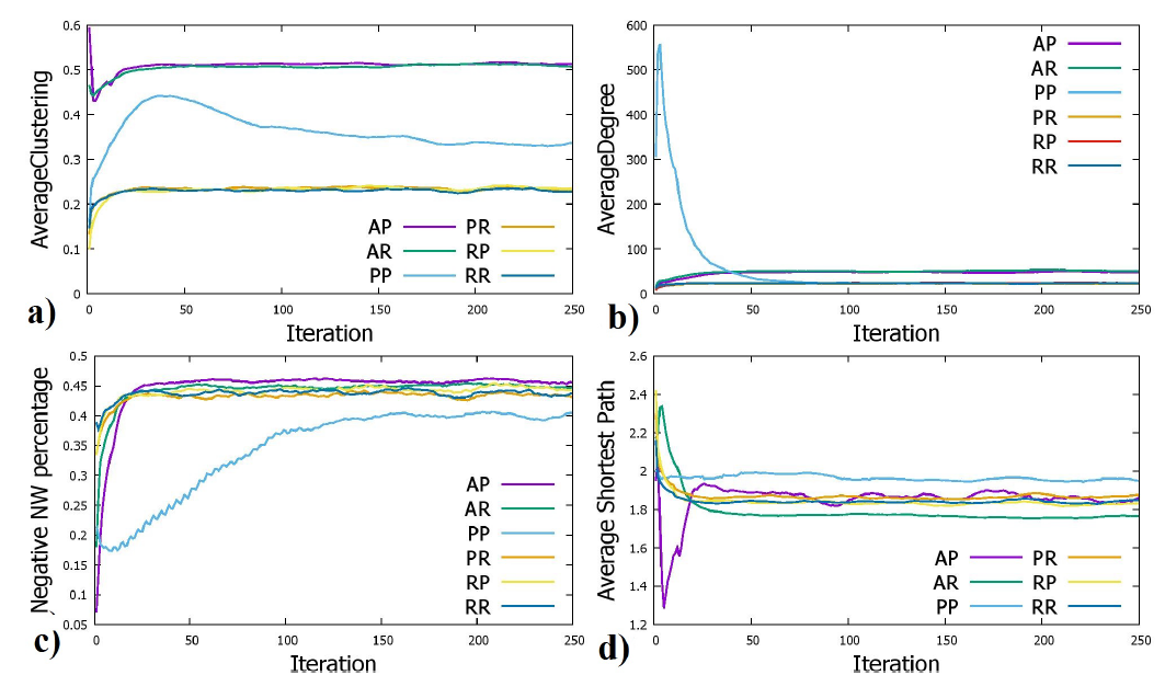
The first set of experiments with a simulation tool showed how it can be used to investigate the interplay of different counter-party choice policies for banks and customers (therefore this scenario considers two driving forces of network evolution). As Figure 3 shows, the topological invariants converge to some certain values as the influence of other parameters on the topological evolution is minimized. In this section, we present results for the share of nodes with negative net worth as a qualitative metric (a number of default banks is not appropriate since the mechanism of nodes elimination is not considered) and three basic topological properties, namely, average degree, clustering coefficient, and average path length, since they are mostly mentioned in empirical interbank networks analyses. The minimum percentage of negative net worth after the stabilization is observed when both policies of banks and customers uses preferential rule (see Figure 3c). Use of this policy also leads to the significantly slower increase of this percentage showing that the system as a whole is more stable. On the other hand, PP policy corresponds to the highest value of an average shortest path (Figure 3d) and the intermediate (in comparison to other policies) values of the average clustering coefficient (Figure 3a). Regarding topological features, average clustering coefficient and average degree are similar to empirical network properties; nevertheless, average path length is the most plausible for preferential algorithms of bank and customer partner choice. This is due to power law topology (which is formed as a result). In addition, this is consistent with the results of (Georg 2013) that networks having more long average shortest path are more stable and show the least number of banks with negative net worth.
One can see that preferential banking policy results in the most stable topology if it is only combined with preferential customer policy (Figure 3c). Therefore, the regulation of only bank choice policy is not sufficient to obtain an optimal network topology. Consequently, regulatory restrictions should be taken in accordance with the current values of system parameters. In addition, regulation should consider that equitable change of a topological property may affect on system resilience to contagion non-linearly (Figure 3a,b). By using the observations on topological metrics during the process of evolution, one can formulate and check hypotheses regarding the interrelation of topological properties, algorithms of counter-party choice, and the resulting stability of an interbank network.
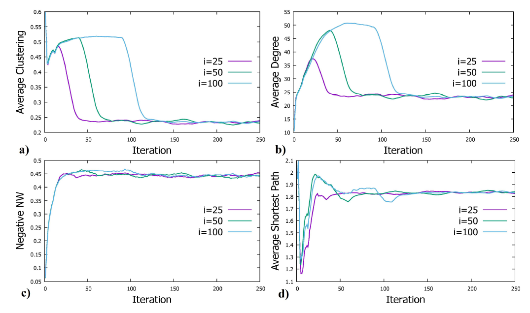
The second set of experiments was intended to show how the simulation tool can be used to study the controllability of an interbank network. The goal of the experiment was to investigate the extent to which the counter-party choice algorithm influences the trajectory of a system state. To explore this, we change these policies at different iterations of simulation (denoted as \(i\)) and compare the resulting trajectories of a system. For the current set of experiments, Figure 4 shows that the evolutionary process could be managed. As Figure 3 shows, the case with assortative policy for banks has average clustering coefficient converging to \(0.5\). When we change this policy to random, the average clustering coefficient changes its trend and stabilizes at \(0.25\) Figure 4a. Similar dynamics is observed for other topological invariants. Using this kind of scenario, one can observe how changing the different algorithms implementing steps 2-4 of general simulation scheme in Figure 1 influences the topological invariants and the resulting stability of a system.
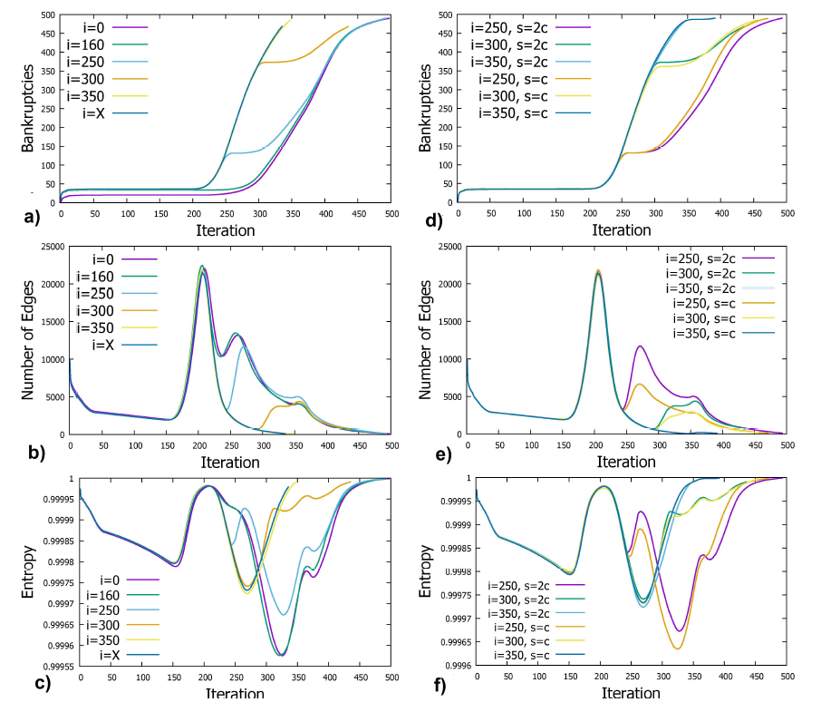
The third set of experiments (Figure 5) demonstrates the case when system evolution is driven by a larger number of parameters (initial graph topology, bank and customer counter-party choice algorithms, rewiring algorithm for failed banks elimination, and fund infusion parameters), resulting in increased unpredictability of the behavior of a system. Figure 5 shows how network evolution is affected by the variation of infusion parameters, iteration and size, for the system with 500 banks and 50000 customers, WS initial topology, and LL rewiring algorithm. Banks choose counter-parties randomly and customers choose them preferentially. The addition of parameters moves the values of graph invariants away from the common trend, they were converging to, since different drivers prevail for different periods of simulation. Figure 5 demonstrates how dynamics may be changed with the modification of parameters in the system under more than two drivers. The chart depicting number of defaults (Figure 5a,d) can be divided into two parts, monotone (where no defaults occur) and increasing, with a tipping point between them. This dynamics can be explained with observations from other charts. A peak in the number of edges (Figure 5b,e) corresponds to a tip in default numbers. In addition, one can observe a sharp increase in the number of edges, 50 iterations before the peak. The reason is that banks tend to create new interbank links to enhance their state. In this way, one can conclude banks worsened after the \(150^{th}\) iteration. After the peak, the number of edges demonstrates dive, which occurs with an increase in the number of defaults and consequently with the number of nodes and edges adjacent to them. Infusion temporally delays the increase in default number, therefore we observe one more peak in the number of edges. It can thus be concluded, that Figures 5a and 5d, with the number of defaults, do not allow to understand the reasons of observed dynamics and single defaults in particular. On contrary, the analysis of topological properties evolution disclose events accompanying default cascades and presents additional information about their reasons.
The increase in the number of driving forces lead the system away from “quasi steady state'' and demonstrates more complex dynamics, which correlates with results presented by (Delli Gatti & Desiderio 2015). The experiment with infusion size (Figure 5) shows that the total amount of funds in the system determines the critical number of edges, which can be created in times of crises (Figure 5b,e). In this way, possible ranges of topological invariants are also restricted according to system properties (Figure 5c,f). A change of infusion iteration, \(\tau_\mathcal{I}\), does not affect a final system state when other parameters are fixed. We specifically observe two states, a better and a worth, with \(\tau_\mathcal{I}\) corresponding to the moment of transition between them (Figure 5a).
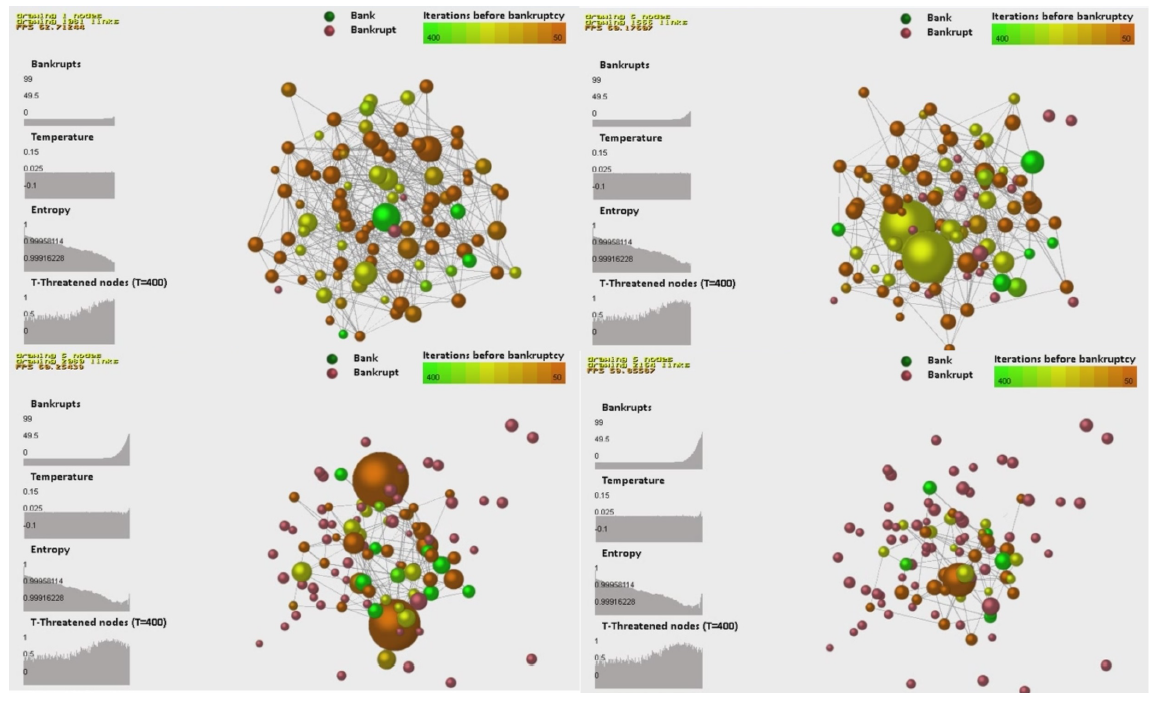
Finally, the data obtained during simulation may be visualized for a more tangible study. This facilitates the detection of reasons of different phenomena observed in the temporal interbank network. The visualization module was implemented to enrich the possibilities of proposed simulation tool. It can be used to visualize the entire process of network evolution with indication of nodes stability and different metrics of network dynamics. The example of visualization of interbank network evolution by means of the visualization module is demonstrated in Figure 6.
Scalability of results
To estimate the computational complexity of a model, one can sum estimates for different steps of simulation as they are performed sequentially. For the algorithms presented, it can be calculated as follows:
| $$O(N_c)+O(N_b^2)+O(N_b)\cdot O\Big(\max\big\{\min\{E_{out};E_{in}\};(N_b-1)^2\big\}\Big)+O(N_b) = O(N_c)+O(N_b^3),$$ |
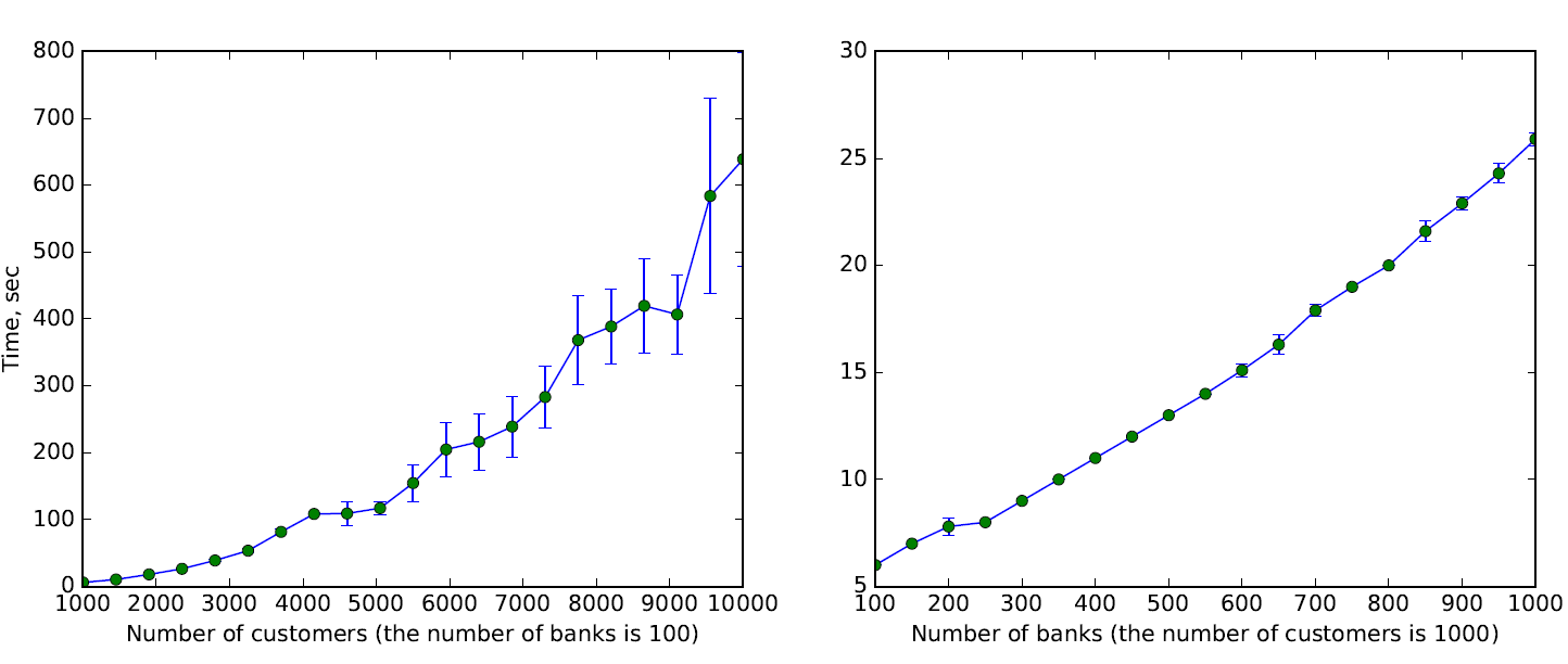
We performed the simulation for the varying number of banks and customers. The results of simulation were averaged by 10 runs. Figure 7 illustrates the execution time of simulation algorithm for the fixed number of banks while varying the number of customers, and for the fixed number of customers with a variation of the number of banks (error bars represent standard deviations). The results demonstrate that the overall execution time of the simulation algorithm for the case of real-world banking networks will be mostly determined by a number of customers. To reduce the execution time of a simulation, a parallel version of simulation algorithm could be introduced.
Conclusion
The paper presents a simulation tool for exploring the evolution of temporal interbank networks affected by several driving forces. Different steps of the general simulation scheme (e.g. counter-party choices or bank elimination) can be implemented in a variety of ways increasing the applicability of the simulation tool. As an example of implementation of the general simulation scheme, we present the model of an interbank network with varying algorithms for: (i) generation of initial topology, (ii) counter-party choice, (iii) rewiring of edges after removing the bank, and (iv) central bank infusion. To support the qualitative and quantitative investigation of simulation results, the proposed tool incorporates static and dynamic topological and stability metrics and the module of visualizing the results of simulation.
The experimental study demonstrates the illustrative example of application of the simulation tool for the synthetic networks under the variation of algorithms (i)-(iv), and shows the results of scalability of the simulation algorithm with an increase of banks and customers. Topological properties were shown to be closely related to other system properties and, therefore, ranges of network invariants can be physically restricted according to them. Thus, bank regulation aiming at optimal network formation should consider these restrictions of a system. In addition, the successful change of a system trajectory can require multiple parameter changes. The mathematical evaluation of the optimal solutions in terms of systemic restrictions and variable number of parameters remains intractable. Our solution allows to observe the simulation of system evolution under different parameter configurations and their values, and evaluate system properties in dynamics.
In the future, we would like to extend this research for evaluation of regulatory restrictions, which are necessary for banks (in combination with other system components) for the formation of resilient network. In addition, further improvement of the tool may include incorporating the existing algorithms for the recovery of the structure of interbank networks using total assets and liabilities as input data (this allows exploring real-world networks) and parallelizing the general simulation scheme in order to reduce the overall simulation time.
Acknowledgements
This research was supported by The Russian Scientific Foundation, Agreement #14–21–00137–Π (02.05.2017). The authors would like to express gratitude to the referees for their careful review and valuable comments which helped to improve the manuscript.Notes
- Also called dynamic networks and time-evolving networks
- Here and further we mean some optimal topology which minimizes loss in the case of financial contagion
- Or follow other more sophisticated relation
- Compared with Laplacian matrix, the adjacency matrix spectrum is not so sufficient, since cospectral matrices demonstrate different topological properties
- We intended the total number of customers per bank to be consistent with empirical results, but we also supposed their number to be proportional to bank total assets (Leonidov & Rumyantsev 2016). Thus, the total number of customers in the system can insignificantly differ from the desired one.
- The Austrian banking system contains about 900 banks (Boss et al. 2004). The Russian banking system, according to data from 1998 to 2004, contains about 900 banks (Vandermarliere 2012), while the Fedwire system contains more than 7,500 participants (Soramäki et al. 2007). At the same time, the e-MID electronic market contains about 200 banks (Iori et al. 2008), and there are 354 banks involved in the Japanese banking system (Inaoka et al. 2004). Opportunities to obtain full data can be restricted; therefore, some studies are based on reduced data or consider networks with the largest banks of a system. (Cajueiro & Tabak 2008) studied interbank networks with 86 banks and 23 non-bank financial organizations, and Montagna and Kok reviewed 50 large EU banks (Montagna & Kok 2013), while (Leonidov & Rumyantsev 2014) considered the Russian inter-bank network with 185 banks for the period from 2011 to 2013. (Delli Gatti et al. 2010) considered 100 banks and 750 firms in their simulations.
- Regarding networks robustness, Boss et al. (2004) argue power-law networks to be more robust to random shocks, on the contrary, Lenzu & Tedeschi (2012b) shown “random financial networks can be more resilient than a power law in case of agents heterogeneity”. Georg (2013) demonstrated “networks with large average path length to be more resilient to financial distress”.
- The increase in rewiring probability (in WS model) lead to decrease in clustering coefficient and average path length. Therefore, small probability is not enough for obtaining small world, since it provides too large average path length. At the same time, there is a range of values, for which clustering is still large while path length is already small. Therefore, these parameters were taken to provide small-world structure and density properties. Network with 100 nodes and k = 4 has appropriate density and at the same time p = 0.6 allows for relatively high clustering coefficient and quite enough average path length.
- Binning and averaging over launches allow to decrease stochastic effects and observe the value, near which fluctuations occur, more clearly. The number of launches and bin size used provide the desired effect and, at the same time, they are not redundant.
Appendix: The visualization of simulation process

The animation demonstrates interbank market evolution until the network disruption resulted from a default cascade. Node diameter corresponds to total asset value of a bank, color represents the number of iterations expected before its default (and shows their remoteness from the critical state). Charts on the left describe the system state and reflect dynamics of the number of failed banks and system characteristics (temperature and entropy of the graph Laplacian and share of nodes in \(\mathscr{T}\)-Threatened set, characterizing changes in node states).
The animation shows there are no defaults in the beginning of modeling but nodes are orange, which is the sign of system instability despite the absence of bankruptcies. In addition, increase in bank assets is uncorrelated with expected moment of default, since this is dynamics of change affecting node remoteness from a critical state. Negative dynamics, observed for the majority of nodes, give rise for default contagion ending with system degeneration.
The charts show the tipping point in the number of failed banks is anticipated by increase in \(\mathscr{T}\)-Threatened set feature, that occur 150 iterations before the cascade. At the same time, topological features considered are more correlated with edge deletion triggered by nodes elimination. In this way, one can notice the consideration of node state dynamics allows for the detection of systemic instabilities caused by node negative dynamics. In current case, this allows for the detection of reasons of ''knock-on effects'' when insignificant financial shock occurs.
References
AHNERT, S. & Fink, T. (2016). Form and function in gene regulatory networks: the structure of network motifs determines fundamental properties of their dynamical state space. Journal of The Royal Society Interface, 13(120), 20160179. [doi:10.1098/rsif.2016.0179]
ALDASORO, I., Delli Gatti, D. & Faia, E. (2015). Bank networks: Contagion, systemic risk and prudential policy. In CESifo Working Paper Series No. 5182. Conference on Endogenous Financial Networks and Equilibrium Dynamics: Addressing Challenges of Financial Stability and Monetary Policy, Banque de France, Paris: Social Science Electronic Publishing. Available at SSRN: http://ssrn.com/abstract=2559722. [doi:10.2139/ssrn.2572877]
ALLEN, F. & Gale, D. (2000). Financial contagion. Journal of Political Economy, 108(1), 1–33. [doi:10.1086/262109]
ARSLAN, I., Caverzasi, E., Gallegati, M. & Duman, A. (2016). Long term impacts of bank behavior on financial stability. an agent based modeling approach. Journal of Artificial Societies & Social Simulation, 19(1), 11: https://www.jasss.org/19/1/11.html. [doi:10.18564/jasss.2964]
BERNANKE, B. S. & Gertler, M. (1995). Inside the black box: The credit channel of monetary policy transmission. Working Paper 5146, National Bureau of Economic Research. [doi:10.3386/w5146]
BOSS, M., Elsinger, H., Summer, M. & Thurner, S. (2004). Network topology of the interbank market. Quantitative Finance, 4(6), 677–684. [doi:10.1080/14697680400020325]
CAJUEIRO, D. O. & Tabak, B. M. (2008). The role of banks in the brazilian interbank market: Does bank type matter? Physica A: Statistical Mechanics and its Applications, 387(27), 6825–6836 [doi:10.1016/j.physa.2008.08.031]
CALEM, P. S. & Mester, L. J. (1995). Consumer behavior and the stickiness of credit-card interest rates. The American Economic Review, 85(5), 1327–1336.
CAPON, N., Fitzsimons, G. J. & Prince, R. A. (1996). An individual level analysis of the mutual fund investment decision. Journal of Financial Services Research, 10(1), 59–82. [doi:10.1007/BF00120146]
CASTIGLIONESI, F. & Eboli, M. (2015). Liquidity flows in interbank networks. Preprint
COHEN-COLE, E., Patacchini, E. & Zenou, Y. (2015). Static and dynamic networks in interbank markets. Network Science, 3(01), 98–123. [doi:10.1017/nws.2015.1]
CONT, R., Moussa, A. & Bastos e Santos, E. (2010). Network structure and systemic risk in banking systems. Available at SSRN: https://papers.ssrn.com/sol3/papers.cfm?abstract_id=1733528.
COX, J. C., Ingersoll Jr, J. E. & Ross, S. A. (1985). A theory of the term structure of interest rates. Econometrica: Journal of the Econometric Society, 53(2), 385–407. [doi:10.2307/1911242]
DELLI Gatti, D. & Desiderio, S. (2015). Monetary policy experiments in an agent-based model with financial frictions. Journal of Economic Interaction and Coordination, 10(2), 265–286. [doi:10.1007/s11403-014-0123-7]
DELLI Gatti, D., Gallegati, M., Greenwald, B., Russo, A. & Stiglitz, J. E. (2010). The financial accelerator in an evolving credit network. Journal of Economic Dynamics and Control, 34(9), 1627–1650. [doi:10.1016/j.jedc.2010.06.019]
DÖRFLER, F., Chertkov, M. & Bullo, F. (2013). Synchronization in complex oscillator networks and smart grids. Proceedings of the National Academy of Sciences, 110(6), 2005–2010. [doi:10.1073/pnas.1212134110]
DOROGOVTSEV, S. N., Goltsev, A. V. & Mendes, J. F. (2008). Critical phenomena in complex networks. Reviews of Modern Physics, 80(4), 1275. [doi:10.1103/RevModPhys.80.1275]
GAI, P., Haldane, A. & Kapadia, S. (2011). Complexity, concentration and contagion. Journal of Monetary Economics, 58(5), 453–470. [doi:10.1016/j.jmoneco.2011.05.005]
GAI, P. & Kapadia, S. (2010). Contagion in financial networks. In Proceedings of the Royal Society of London A: Mathematical, Physical and Engineering Sciences, (p. rspa20090410). The Royal Society.
GEORG, C.-P. (2013). The effect of the interbank network structure on contagion and common shocks. Journal of Banking & Finance, 37(7), 2216–2228. [doi:10.1016/j.jbankfin.2013.02.032]
GOODHART, C., Hofmann, B. & Segoviano, M. (2004). Bank regulation and macroeconomic fluctuations. Oxford Review of Economic Policy, 20(4), 591–615. [doi:10.1093/oxrep/grh034]
GOROCHOWSKI, T. E., di Bernardo, M. & Grierson, C. S. (2009). Netevo: A computational framework for the evolution of dynamical complex networks. arXiv preprint arXiv:0912.3398: https://arxiv.org/abs/0912.3398.
GRILLI, R., Tedeschi, G. & Gallegati, M. (2015). Markets connectivity and financial contagion. Journal of Economic Interaction and Coordination, 10(2), 287–304. [doi:10.1007/s11403-014-0129-1]
GULEVA, V. Y. (2016a). The combination of topology and node states dynamics as an early-warning signal of critical transition in a banking network model. Procedia Computer Science, 80, 1755–1764. International Conference on Computational Science (ICCS 2016), 6–8 June 2016, San Diego, California, USA. [doi:10.1016/j.procs.2016.05.436]
GULEVA, V. Y. (2016b). Dynamic interbank network simulator. https://www.openabm.org/model/5285/version/1/view. Accessed: 2017–07–07.
GULEVA, V. Y., Amuda, A. & Bochenina, K. (2016). The impact of network topology on banking system dynamics. Communications in Computer and Information Science, 674, 596–599. Digital Transformation & Global Society (DTGS 2016), 23–24 July 2016, Saint-Petersburg, Russia. [doi:10.1007/978-3-319-49700-6_59]
GUPTA, A., King, M. M., Magdanz, J., Martinez, R., Smerlak, M. & Stoll, B. (2013). Critical connectivity in banking networks. SFI CSSS. SFI CSSS report: http://samoa.santafe.edu/media/cms_page_media/500/Banks_SFI_report%20(1).pdf.
HALAJ, G. & Kok, C. (2015). Modelling the emergence of the interbank networks. Quantitative Finance, 15(4), 653–671. [doi:10.1080/14697688.2014.968357]
HALDANE, A. G. & May, R. M. (2011). Systemic risk in banking ecosystems. Nature, 469(7330), 351–355. [doi:10.1038/nature09659]
HALDANE, A. G. et al. (2009). Rethinking the financial network. Speech delivered at the Financial Student Association, Amsterdam, April, (pp. 1–26).
INAOKA, H., Ninomiya, T., Taniguchi, K., Shimizu, T., Takayasu, H. et al. (2004). Fractal network derived from banking transaction–an analysis of network structures formed by financial institutions. Bank Jpn Work Pap, 4: https://www.boj.or.jp/en/research/wps_rev/wps_2004/data/wp04e04.pdf.
IORI, G., De Masi, G., Precup, O. V., Gabbi, G. & Caldarelli, G. (2008). A network analysis of the italian overnight money market. Journal of Economic Dynamics and Control, 32(1), 259–278. [doi:10.1016/j.jedc.2007.01.032]
IORI, G., Mantegna, R. N., Marotta, L., Micciche, S., Porter, J. & Tumminello, M. (2015). Networked relationships in the e-mid interbank market: A trading model with memory. Journal of Economic Dynamics and Control, 50, 98–116. Crises and Complexity Research Initiative for Systemic Instabilities (CRISIS) Workshop 2013. [doi:10.1016/j.jedc.2014.08.016]
KIM, D. H. & Singleton, K. J. (2012). Term structure models and the zero bound: an empirical investigation of japanese yields. Journal of Econometrics, 170(1), 32–49. [doi:10.1016/j.jeconom.2011.12.005]
KRAUSE, A. & Giansante, S. (2012). Interbank lending and the spread of bankfailures: A networkmodel of systemic risk. Journal of Economic Behaviour & Organization, 83(3), 583–608. [doi:10.1016/j.jebo.2012.05.015]
LARIONOVA, N. & Varlamova, J. (2014). Correlation analysis of macroeconomic and banking system indicators. Procedia Economics and Finance, 14, 359–366 [doi:10.1016/S2212-5671(14)00724-2]
LENZU, S. & Tedeschi, G. (2012a). Systemic risk on different interbank network topologies. Physica A: Statistical Mechanics and its Applications, 391(18), 4331–4341. [doi:10.1016/j.physa.2012.03.035]
LENZU, S. & Tedeschi, G. (2012b). Systemic risk on different interbank network topologies. Physica A: Statistical Mechanics and its Applications, 391(18), 4331–4341. [doi:10.1016/j.physa.2012.03.035]
LEONIDOV, A. & Rumyantsev, E. (2014). Systemic interbank network risks in Russia. arXiv preprint arXiv:1410.0125: https://arxiv.org/abs/1410.0125.
LEONIDOV, A. & Rumyantsev, E. (2016). Default contagion risks in russian interbank market. Physica A: Statistical Mechanics and its Applications, 451, 36–48. [doi:10.1016/j.physa.2015.12.130]
LIU, S., Perra, N., Karsai, M. & Vespignani, A. (2014). Controlling contagion processes in activity driven networks. Physical review letters, 112(11), 118702. [doi:10.1103/PhysRevLett.112.118702]
LUX, T. (2015). Emergence of a core-periphery structure in a simple dynamic model of the interbank market. Journal of Economic Dynamics and Control, 52, A11–A23. [doi:10.1016/j.jedc.2014.09.038]
LUX, T. (2016). A model of the topology of the bank–firm credit network and its role as channel of contagion. Journal of Economic Dynamics and Control, 66, 36–53. [doi:10.1016/j.jedc.2016.03.002]
MERRIS, R. (1998). Laplacian graph eigenvectors. Linear algebra and its applications, 278(1-3), 221–236. [doi:10.1016/S0024-3795(97)10080-5]
MOHAR, B., Alavi, Y., Chartrand, G. & Oellermann, O. (1991). The Laplacian spectrum of graphs. Graph theory, combinatorics, and applications, 2(871-898), 12.
MONTAGNA, M. & Kok, C. (2013). Multi-layered interbank model for assessing systemic risk. Kiel Working Paper, (1873), 1–53: http://econpapers.repec.org/paper/zbwifwkwp/1873.html.
NIER, E., Yang, J., Yorulmazer, T. & Alentorn, A. (2007). Network models and financial stability. Journal of Economic Dynamics and Control, 31(6), 2033–2060. [doi:10.1016/j.jedc.2007.01.014]
QUAX, R., Bader, D. A. & Sloot, P. M. (2011). Seecn: Simulating complex systems using dynamic complex networks. International Journal for Multiscale Computational Engineering, 9(2). [doi:10.1615/IntJMultCompEng.v9.i2.50]
RAHMAN, M. A., Pakštas, A. & Wang, F. Z. (2009). Network modelling and simulation tools. Simulation Modelling Practice and Theory, 17(6), 1011–1031. [doi:10.1016/j.simpat.2009.02.005]
ROBERTSON, D. A. (2003). Agent-based models of a banking network as an example of a turbulent environment: the deliberate vs. emergent strategy debate revisited. Emergence, 5(2), 56–71. [doi:10.1207/S15327000EM050207]
ROUKNY, T., Bersini, H., Pirotte, H., Caldarelli, G. & Battiston, S. (2013). Default cascades in complex networks: Topology and systemic risk. Scientific reports, 3, 2759. [doi:10.1038/srep02759]
SCHAUL, J. (2011). ComplexNetworkSim a python package for the simulation of agents connected in a complex network: http://pythonhosted.org/ComplexNetworkSim/. Accessed: 2016–10–31.
SIDDIQUE, M. et al. (2012). Bank selection influencing factors: A study on customer preferences with reference to rajshahi city. Asian Business Review (ABR), 1(1), 2304–2613.
SLOOT, P. & Erenstein, A. (2009). DynaNets for dynamically changing complex networks: http://www.dynanets.org/home.html. Accessed: 2016–10–31.
SMAGA, P., Wiliński, M., Ochnicki, P., Arendarski, P. & Gubiec, T. (2016). Can banks default overnight? Modeling endogenous contagion on o/n interbank market. arXiv preprint arXiv:1603.05142: https://arxiv.org/abs/1603.05142.
SORAMÄKI, K., Bech, M. L., Arnold, J., Glass, R. J. & Beyeler, W. E. (2007). The topology of interbank payment flows. Physica A: Statistical Mechanics and its Applications, 379(1), 317–333. [doi:10.1016/j.physa.2006.11.093]
STEINBACHER, M., Steinbacher, M. & Steinbacher, M. (2016). Robustness of banking networks to idiosyncratic and systemic shocks: a network-based approach. Journal of Economic Interaction and Coordination, 11(1), 95–117. [doi:10.1007/s11403-014-0143-3]
TAMBAYONG, L. (2009). Review of Dynamical Processes on Complex Networks. The Journal of Artificial Societies and Social Simulation, 12(3): https://www.jasss.org/12/3/reviews/tambayong.html.
UPPER, C. (2011). Simulation methods to assess the danger of contagion in interbank markets. Journal of Financial Stability, 7(3), 111–125. [doi:10.1016/j.jfs.2010.12.001]
VANDERMARLIERE, B. (2012). Network analysis of the russian interbank system. Master of science thesis at the Gent University: http://lib.ugent.be/fulltxt/RUG01/001/892/466/RUG01-001892466_2012_0001_AC.pdf.
XIANG, X., Kennedy, R., Madey, G. & Cabaniss, S. (2005). Verification and validation of agent-based scientific simulation models. In Agent-Directed Simulation Conference, (pp. 47–55): http://www.cse.nd.edu/~nom/Papers/ADS019_Xiang.pdf.
YE, C., Torsello, A., Wilson, R. C. & Hancock, E. R. (2015). ‘Thermodynamics of time evolving networks.’ In Jolion, J.-M. & Kropatsch, W. G. (eds.), Graph-Based Representations in Pattern Recognition, (pp. 315–324).Wien: Springer. [doi:10.1007/978-3-319-18224-7_31]