
Introduction
Iterative Proportional Fitting (IPF) is a popular and well-established technique for generating synthetic populations from marginal data. Compared with other methods of population synthesis, IPF is relatively fast, simple and easy to implement, as showcased in a practical introduction to the subject by Lovelace & Dumont ( 2016). Furthermore, a number of software packages aimed at facilitating IPF for spatial microsimulation and other applications have been published such as Barthelemy & Suesse (2016) and Jones et al. ( 2016).
However, the method has various limitations from the perspective of social simulation via agent-based models: IPF generates fractional weights instead of integer populations (an issue that can be tackled by integerisation); handles empty cells poorly (Lovelace et al. 2015); and requires a representative individual-level ‘seed’ population. These issues and the mathematics underlying them are explored in Založnik (2011).
Integerisation is only a partial solution to the issue of fractional weights. Whilst algorithms for integerisation such as ‘truncate replicate sample’ maintain the correct overall population, the adjustments can create a mismatch between the original and simulated marginal data (Lovelace & Ballas 2013). Using IPF-generated probabilities as a basis for a sampling algorithm is an alternative solution but again care must be taken to correctly match the marginal distributions and generate a realistic population.
In this paper we investigate sampling techniques where a synthetic population is built exclusively in the integer domain. The research reported in this paper forms part of, and is partly motivated by, a larger body of work in which there is a requirement to generate individual simulated agents for an entire city. In the larger project, the ultimate goal is to impute journey patterns to each member of the simulated population using app-based mobility traces in order to generate travel demand schedules for an entire urban population in pseudo-real-time.
The motivation behind the development of this method came from the fact that IPF, in general, does not generate integral populations in each state. If the resulting population is used as a basis for Agent-Based Modelling (ABM), then some form of integerisation process must be applied to the synthesised population. Whilst this process preserves the overall population, it may not exactly preserve all of the marginal distributions. Although the integerisation process may not introduce significant errors, the authors considered whether there was an alternative method of synthesis that would directly result in an integral population that exactly matched the marginal distributions.
We could not find any references in the literature on the use of quasirandom sequences for the purpose of population synthesis, and so decided to investigate the suitability of sampling algorithms using such sequences.
Working exclusively in the integer domain requires that marginal frequencies are integral. Often, these are expressed as probabilities rather than frequencies. We propose that integerising each marginal at this stage is preferable to integerising the final population. Mathematically, integerisation in a single dimension is straight-forward and a demonstrably optimal (i.e. closest) solution can always be reached.
We first show that by using without-replacement sampling guarantees that the randomly sampled population will exactly match the marginal data. We then compare the statistical properties of populations sampled using pseudo- and quasirandom numbers showing that the quasirandom sampling technique provides far better degeneracy, achieving solutions closer to the maximal entropy solution that IPF converges to.
Theory
In this section we first quantitatively describe the core concepts that comprise the sampling technique. We then formally state the problem that the technique is used to solve, and finally define the statistical metrics that we use for assessing and comparing the results.
Quasirandom numbers
Quasirandom numbers, often referred to as low discrepancy sequences, are preferential to pseudorandom numbers in many applications, despite not having some of the (appearance of) randomness that good pseudorandom generators possess. In this work we focus on the Sobol quasirandom sequence (Sobol’ 1967) with subsequent implementation and refinement by Bratley & Fox (1988) and Joe & Kuo (2003).
To compare and contrast quasirandom and pseudorandom numbers, we use the MT19937 variant of the Mersenne Twister pseudorandom generator (Matsumoto & Nishimura 1998).
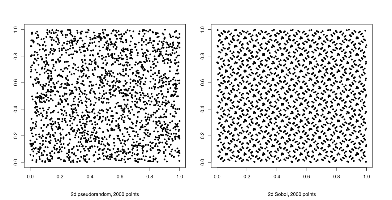
Figure 1 qualitatively illustrates the difference between pseudo- and quasirandom sampling. Each plot contains 2000 uniform points in two dimensions. The quasirandom samples fill the sample space far more evenly and display an obvious lack of randomness, clearly showing a lack of independence between samples. In contrast, the pseudorandom samples show no discernible pattern with clusters and gaps present in the sampling domain, suggesting independence between variates.
Sobol sequences, as with other quasirandom sequences, have an inherent dimensionality and a relatively short period - the sequence is exhausted once every integer in the sample space has been sampled. Successive samples evenly fill the sample space, and thus lack independence. Conversely, a good pseudorandom generator has no discernible dependence between variates often has a much longer period, allowing for very large samples to be taken.
For applications such as numerical integration, Sobol sequences converge at a rate of \(\approx1/N\) (more accurately \((ln N)^D/N\), Press et al.1992) compared to \(\approx1/\sqrt N\) for a pseudorandom generator, and thus require far fewer samples to achieve the same level of accuracy. This makes quasirandom sampling particularly suitable for Monte-Carlo integration of high-dimensional functions: far fewer samples are required to obtain the same level of accuracy that would be achieved using pseudorandom sampling.
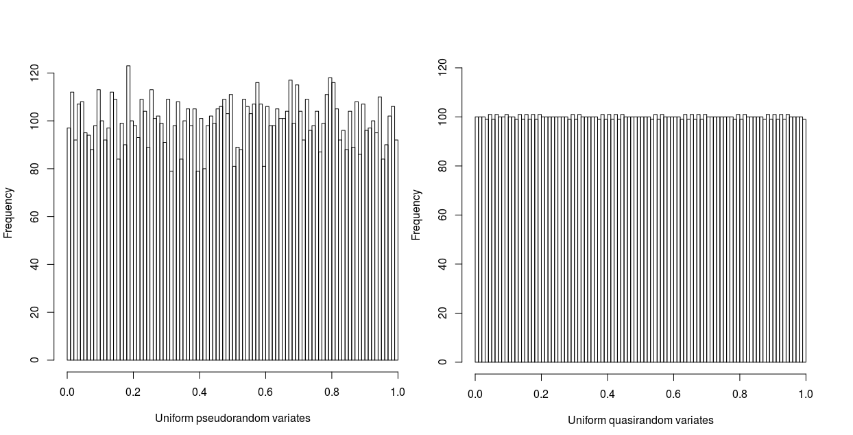
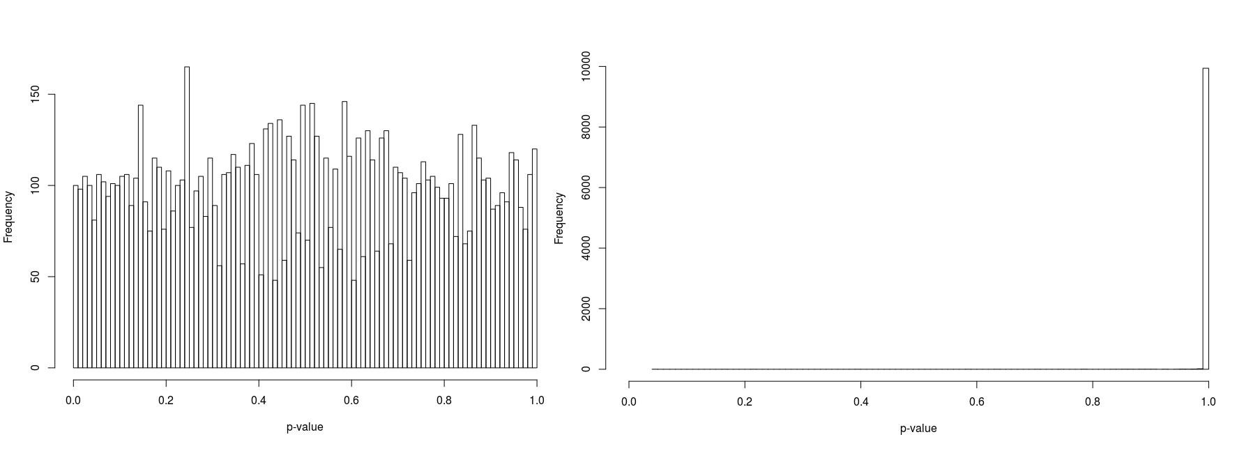
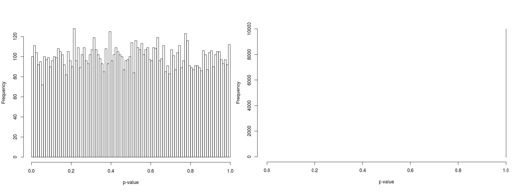
Figure 2 illustrates the superior convergence of quasirandom numbers. The histograms contain 10000 samples in 100 bins, and clearly the quasirandom sequence is far closer to the true distribution. Furthermore, consider the following simple example: we wish to calculate the expected value of the sum of 2 fair and independent dice, sampling 100 times. Using pseudorandom sampling, with a standard error proportional to the square root of the number of samples, we would expect to get an estimate of \(7 \pm 10\%\). However, using quasirandom sampling, since the standard error [1] is inversely proportional to the number of samples, the estimate will be \(7 \pm 1\%\). To achieve the same level of accuracy with pseudorandom numbers would require 10000 samples.
Quasirandom sequences are not seeded like pseudorandom generators. To avoid repetition, and for better degeneracy, it is recommended to discard a number of variates on initialisation (Joe & Kuo 2003), and on subsequent sampling continue the sequence from its previous position.
When using quasirandom sequences it is extremely important to ensure that every sample is used. Discarding a subset of the samples will potentially destroy the statistical properties of the entire sequence. For this reason quasirandom sequences must not be combined with rejection sampling methods, which are often used to convert the ‘raw’ uniformly-distributed variates into e.g. normally-distributed ones.
Sampling without replacement
Given a discretely distributed population \(P\) of individuals which can be categorised into one of \(n\) states, each with integral frequencies \(\{f_1,f_2,...f_n\}\), a random sample \(i \in \{1...n\}\) has probability
| $$p_i = \frac{f_i}{\sum\limits_{k=1}^{n}f_k}$$ |
Since \(f_i\) cannot be oversampled, this implies that all the other states \(f_{j\neq{i}}\) cannot be collectively undersampled. By extension, if all but one states \(f_{i\neq{j}}\) cannot be oversampled, then \(f_j\) cannot be undersampled. Thus each state can neither be under- nor oversampled: the distribution must be matched exactly.
Extending this to two dimensions is straightforward: given marginal frequency vectors \(\mathbf{f}\) and \(\mathbf{g}\), each summing to \(P\) and (for argument's sake) of length \(n\), take a random two dimensional sample \((i,j) \in \{1...n\}^2\) with probability
| $$p_{i,j} = \frac{f_{i}g_{j}}{\sum\limits_{k=1}^{n}f_k\sum\limits_{k=1}^{n}g_k}$$ |
| $$\begin{split} f_i \leftarrow f_i-1 \\ g_j \leftarrow g_j-1 \end{split}$$ |
Integerisation of probabilities
Given a vector of discrete probabilities \(p_i\) for each state in a single category, and an overall population \(P\), the nearest integer frequencies \(f_i\) can be obtained using the following algorithm: firstly obtain a lower bound for integer frequencies by computing
| $$\begin{split} f_i = \lfloor p_{i}P \rfloor \\ g_i = p_i P - f_i \\ X = P - \sum\limits_i{f_i} \end{split}$$ | (4) |
| $$\begin{equation} \sum\limits_i{f_i} = P \end{equation}$$ | (5) |
Problem statement
Population synthesis (Orcutt 1957) refers to the (re)generation of individual-level data from aggregate (marginal) data. For example, UK census data provides aggregate data across numerous socioeconomic categories at various geographical resolutions - but it expressly does not provide data at an individual-level, for privacy reasons among others. Only the most basic form of microsynthesis is described here - that where only the marginal data governs the final population, and no exogenous data is supplied. This corresponds to the use of IPF with a unity seed.
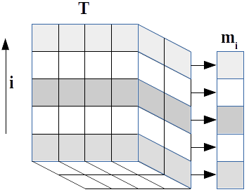
A mathematical statement of the problem is as follows:[2] we wish to generate a population \(P\) of individuals which can be characterised into \(D\) separate categories, each of which can occupy \(l\) discrete states. Each category is represented by a known frequency vector \(\mathbf{m}_i\) of length \(l_i\) giving the marginal occurrences of a state within a single category. Thus we have \(S\) possible overall states
| $$S=\prod\limits_{i=1}^{D}l_i$$ | (6) |
| $$\sum\limits_{\mathbf{k}, k_i fixed} \mathbf{T}_\mathbf{k} = \mathbf{m}_i \label{eqn:margins}$$ | (7) |
Each marginal sum and the sum of the elements of contingency table must equal the population P:
| $$\sum\limits \mathbf{m}_{i} = \sum\limits_\mathbf{k} \mathbf{T} = P $$ | (8) |
| $${\mathbf{T} \in \mathbb{N}^S,\mathbf{m}_i} \in \mathbb{N}^{l_i}$$ | (9) |
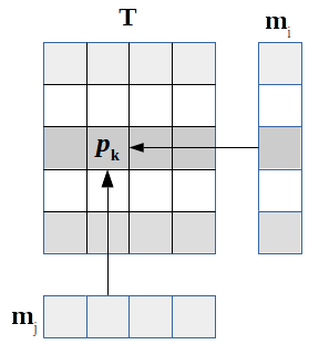
The probability of a given state k being occupied is thus the product of the marginal probabilities:
| $$p_{\mathbf{k}} = \prod\limits_{i=1}^{D}(\mathbf{m}_i)_\mathbf{k}/P $$ | (10) |
The degrees of freedom \(d\) of the system (required in order to calculate the statistical significance of the population) is given by
| $$d=\prod\limits_{i=1}^{D}(l_i-1)$$ | (11) |
Degeneracy, Entropy and Statistical Likelihood
In this work we use the term degeneracy to mean the number of possible different ways a given overall population \(P\) can be sampled into a \(D\)-dimensional table \(\mathbf{T}\) containing \(S\) possible states \(\mathbf{k}\), with occupancy probability \(p_\mathbf{k}\), the system having \(d\) degrees of freedom. In this sense, the term degeneracy is closely related to (information-theoretic) entropy: a high-degeneracy state can be considered a high-entropy state, and a low-degeneracy state a low-entropy one.
Assuming that the marginal distributions are uncorrelated, then the higher the degeneracy/entropy of the population, the more statistically likely the population is. We measure the statistical likelihood of populations using a \(\chi^2\) statistic:
| $$\chi^2 = \sum\limits_{\mathbf{k}}\frac{(\mathbf{T}_\mathbf{k}-p_\mathbf{k}P)^2}{p_\mathbf{k}P}$$ | (12) |
| $$\text{p-value}=1-F(d/2,\chi^2)$$ | (13) |
The purpose in this context is to use these metrics to demonstrate the ability of the sampling method described here to generate populations with a high p-value, i.e. high degeneracy, high entropy, high likelihood and low statistical significance.
The Algorithm
This section describes the Quasirandom Integer Without-replacement Sampling (QIWS) algorithm. A commentary on the process by which we arrived at this algorithm follows in the Discussion.
The inputs required for the algorithm to operate are simply a number of integer vectors defining the marginals. The elements of each vector must sum to the same value, satisfying the population constraint defined earlier.
Given a valid input of \(D\) marginal vectors \(\mathbf{m}_i\), the process then proceeds as follows:
- Create a \(D\)-dimensional discrete without-replacement distribution using the marginals \(\mathbf{m}_i\).
- Sample \(P\) random variates from this distribution to create a population \(\mathbf{T}\). Specifically, we sample a value of \(\mathbf{k}\) and increment the value of \(\mathbf{T}_\mathbf{k}\), repeating until the distribution is fully depleted. Constructing the problem in this way automatically ensures that all constraints are automatically met, as explained in the previous section
- Compute occupation probabilities \(p_\mathbf{k}\) for each state \(\mathbf{k}\)
- Compute a \(\chi^2\) statistic and a p-value, which represents the statistical significance of the synthetic population (in this case we prefer higher p-values, i.e. statistically insignificant populations).
The implementation
The algorithm is implemented in an R package called humanleague. A description of the technical implementation details can be found in the Appendix. The package is open source under a GPL licence and available at https://github.com/CatchDat/humanleague.
In order to use the microsynthesis function, the input data requirements are a number of discrete integer marginal distributions, i.e. counts of population in each state of some category. If any marginal data is expressed as probabilities, a function is provided to convert these to integer frequencies. For reference, we also provide a function for direct generation of Sobol sequences.
Usage examples
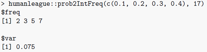
\(\texttt{prob2IntFreq}\): this function converts an array of discrete probabilities \(p_i\) into integral frequencies, given an overall population \(P\). It also returns the mean square error between the integer frequencies and their unconstrained values \(p_iP\).
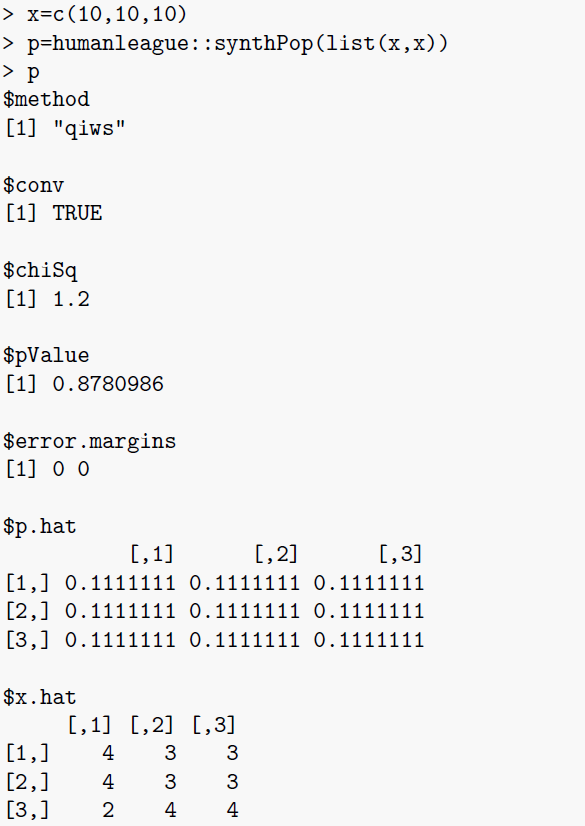
\(\texttt{synthPop}\): This is function that performs the microsynthesis. The function supports dimensionalities up to 12, although this limit is arbitrary and could be increased if necessary. Input is simply a list of (between 2 and 12) integer vectors representing the marginals. Marginal vectors must all sum to the population (to satisfy the population constraint) \(P\). The output is broadly compatible with the established \(\texttt{mipfp}\) (Barthelemy & Suesse 2016) R package:
- \(D\)-dimensional population table \(\mathbf{T_\mathbf{k}}\)
- \(D\)-dimensional occupancy probability array \(\mathbf{p_\mathbf{k}}\)
- boolean value indicating convergence
- maximum value of each residual vector
- \(\chi^2\) statistic
- p-value
This is illustrated by the example output below:
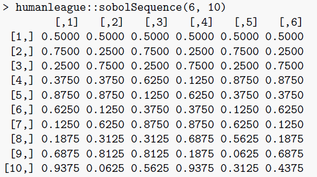
sobolSequence: this function simply produces a Sobol sequence of the requested dimension and length, optionally skipping part of the sequence. The example below produces the first ten values of the six-dimensional sequence, without skipping.
Comparison to Existing Methods
Statistical properties
Using IPF with a unity seed is equivalent to populating each state proportionally to the probability of occupancy of the state. This solution maximises entropy (Lovelace et al. 2015). Sampling algorithms generally cannot achieve the same entropy since they only populate states with integer populations.
We assume that high-entropy populations are preferable for most applications and aim in this section is to show that quasirandom sampling is much better at achieving high-entropy populations than pseudorandom sampling.
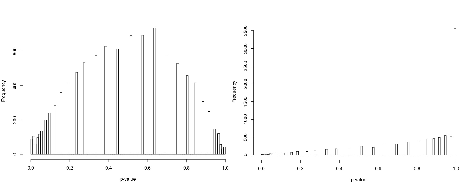
In order to compare psuedorandomly-sampled and quasirandomly sampled populations, we considered a two-dimensional test case in which each marginal had ten equally probable states. We varied the total population resulting in population densities (average population per state) of 1, 3, 10 and 100. For each case we recorded the p-value for 10000 populations. Histograms of the p-values are illustrated in Figure 5 to 8.
Performance
Since computers vary widely in performance for many reasons, we present performance values normalised to the execution time of QIWS for the first test case. For reference, the hardware used was a recent, fairly standard desktop PC and the performance test run times (for 1000 tests) were of the order of seconds.
The test timing results are summarised in Table 1 for a number of theoretical and more realistic test cases.

Discussion
Evolution of the algorithm
Firstly, it was demonstrated that naive pseudorandom sampling could not reliably generate populations matching the marginals. Since successive samples are ostensibly independent, there is no mechanism to prevent under- or oversampling of any particular state.
The initial algorithm simply sampled the marginal distributions (with replacement), using quasirandom numbers, to build a population. For “toy” problems this method often worked, but for more complex problems the algorithm often failed to exactly match all the marginals.
| Pop | States | QIWS | IPF |
| 20 | 4 | 1.0 | 66.3 |
| 125 | 25 | 1.3 | 96.7 |
| 935 | 49 | 2.3 | 68.3 |
| 4958 | 16032 | 30.7 | 1559.3 |
| 4098 | 11760 | 23.0 | 1069.0 |
| 4029 | 11904 | 22.7 | 1027.3 |
| 4989 | 14640 | 28.3 | 1457.0 |
| 5219 | 15168 | 28.7 | 1557.7 |
In general, the resulting population mismatched the marginals only slightly. A correction algorithm was implemented which, applied at most once for each dimension of the population, adjusted the states by the error in the marginal for that dimension.
It was also demonstrated that a correction step as described above could not be applied to a pseudorandomly generated population because the marginal errors were almost always too large to be able to apply a correction: such corrections would typically result in a negative population in one or more states.
Furthermore, it was shown that even using quasirandom sampling, it was not always guaranteed that a population could be corrected using the method described above without a negative population in one or more states. The sparser (the ratio of the total population P to the number of possible states S) the population, the more often this would occur. Often the solution was simply to discard and resample the population until an exact or correctable population was generated. This raised a concern about the reliability (and efficiency) of the algorithm, and in fact further testing did reveal cases where the algorithm the number of resamples required was unacceptably large, even exhausting the period of the generator.
This flaw drove the authors to develop an alternative formulation of the algorithm, and it transpired that without-replacement sampling would guarantee that the population matched all marginals by design (as explained in section 2.9, eliminating the need for the correction step entirely. In fact, this method is guaranteed to work regardless of the choice of underlying random number generation.
The next phase of the work was to analyse generated populations statistically, focussing on the statistical likelihood of the resulting populations in order to determine whether quasirandom sampling offers any additional benefit. The results from this work, presented in the previous section, are discussed below.
Statistical properties
Randomness in context
To put pseudorandom versus quasirandom sampling into context, and to explain at least intuitively[3] why we observe different distributions of p-values (Table 5 to 8), firstly consider a ‘random’ number generator that simply always returns zero. If we used this as the basis for without-replacement sampling of a marginal distribution \(\lbrace30,30,30\rbrace\), we would get a sequence consisting of ten ones, ten twos and ten threes as the samples exhausted each bin and moved to the next. In two dimensions, this would result in a population matrix
| $$\left( \begin{array}{ccc} 30 & 0 & 0 \\ 0 & 30 & 0 \\ 0 & 0 & 30 \end{array} \right)$$ |
Simplifying Equation 12 for this example, and assuming a variation \(X\) in the populations of each state (from their expected value), we can thus estimate \(\chi^2\) as
| $$\chi^2 = \frac{N^2}{P}X^2$$ | (14) |
Now, repeating the sampling process using a good-quality pseudorandom number generator, given that convergence is inversely proportional to the square root of the number of samples, we would typically expect a population matrix more like
| $$\left( \begin{array}{ccc} 10\pm3 & 10\pm3 & 10\pm3 \\ 10\pm3 & 10\pm3 & 10\pm3 \\ 10\pm3 & 10\pm3 & 10\pm3 \end{array} \right)$$ |
| $$\chi^2 \approx \frac{N^2}{P}\frac{P}{N}=N$$ |
Repeating again, this time using a quasirandom sequence and bearing in mind that convergence is now linear, a typical population matrix would be
| $$\left( \begin{array}{ccc} 10\pm1 & 10\pm1 & 10\pm1 \\ 10\pm1 & 10\pm1 & 10\pm1 \\ 10\pm1 & 10\pm1 & 10\pm1 \end{array} \right)$$ |
| $$\chi^2 \approx \frac{N^2}{P}$$ | (16) |
This result, whilst not mathematically rigorous - the analysis is complicated by the use of without-replacement sampling - is in line with the sampled uniform distributions shown in Figure 2. We believe that this example goes some way to explaining the histograms given in Figure 5 to 8.
Furthermore, the figures seem to suggest that whilst pseudorandomly-sampled populations converge to an even distribution of p-values (i.e. there is no bias towards high-entropy populations) as the population density increases, quasirandomly-sampled populations strongly converge to populations with a unity p-value. The latter is clearly preferable when the marginals are meant to be independent, confirming the null hypothesis.
For low population densities, there is evidence of ‘quantisation’ of the p-value distribution, this is thought to arise from the fact that for sparse populations, there are fewer possible configurations of the population. Why there is an apparent bias towards p-values around 0.5 for pseudorandomly sampled sparse populations is unclear to us.
Statistical likelihood
The minimum \(\chi^2\) value possible from a sampled integral population is generally greater than zero simply due to the fact that the expected population in each state may not be integral. Thus a p-value of exactly unity is not always possible.
As explained is the previous section, QIWS has a strong bias towards high p-values but may nevertheless produce statistically unlikely populations. The \(\chi^2\) and p-value that are supplied along with the population should be checked against some suitable threshold, resampling as necessary.
Performance
QIWS performance in terms of computational efficiency is far superior to the IPF implementation we compared it to. One reason for this is that QIWS is not iterative, but the following points should also be noted:
- the comparison is somewhat unfair since our implementation is compiled C and C++ code and Ipfp’s implementation is interpreted R code.
- performance of population synthesis may not be a significant factor in most workflows, and thus speed may be of marginal advantage. However in large-scale ensemble simulation applications, the performance of QIWS may be an advantage.
Application / range of use
For agent-based modelling (ABM) applications, QIWS has the advantage that it only generates integer populations. Thus integerisation, which may alter the population in such a way that the marginals are no longer met, is not required.
An alternative to integerisation is sampling. Such techniques have been documented, although none mention the use of quasirandom sampling. For example, in the doubly-constrained model described in Lenormand et al. (2016), they use a fractional population generated with IPF as a joint distribution from which to randomly sample individuals. In Gargiulo et al. (2012) without-replacement sampling is also used with the joint distribution dynamically updated after each sample.
IPF can be used for microsimulation in cases where some marginal data is not fully specified. For example, some categorical constraint data may only be available for a subset of the whole population. By using this data as a seed population, rather than as a marginal constraint, the incomplete data is scaled to, and smoothed over, the overall population. This type of microsimulation is described and discussed in the “CakeMap” example in Lovelace & Dumont (2016).
The authors believe that the current implementation of QIWS could be extended to deal with problems such as “CakeMap” or more generally ones where some exogenous data must be taken into account. The approach would be to construct a dynamic joint distribution from marginal and exogenous data, updating as each sample is taken.
With given marginals and seed population, IPF will always result in the same overall population. QIWS differs in this respect in that the same inputs can be used to generate multiple different populations, all of which meet the marginal constraints. These could potentially used in an ensemble simulation to test the sensitivity of a model to different synthetic populations generated from the same marginal data.
QIWS may potentially be of use in the process of anonymisation by microsynthesising aggregate data from a known population. It is outside the scope of this work, but since full marginal data will likely be available, its use in this context may be worth investigating.
Conclusion
This work forms part of a larger project in which a city-scale population microsynthesis is used as the basis for an Agent-Based Model of commute patterns, using census data combined with a crowdsourced dataset. The QIWS algorithm and the so ware implementation in an R package was developed for this purpose, eliminating the need for integerising the synthesised population. This microsimulation involved categorical variables (i.e. marginals) representing home and work locations (at MSOA resolution), mode of transport, gender, age group, and economic activity type, with the crowdsourced data overlaid on the larger census population.
Our analysis shows that quasirandom sampling results in more statistically likely populations than pseudo-random sampling as illustrated in the histograms in Table 5 to 8. The statistical likelihood/significance of the sampled population may vary and thus metrics are provided to guide the user in determining the suitability of the generated population.
In situations where integral populations with high statistical likelihood are desirable QIWS presents an advantage over established techniques by either eliminating the need for integerisation, or by its use of quasirandom sequences to create high-entropy sampled populations.
In its current implementation, QIWS is more limited in scope than IPF in that it is unable to deal with cases where some marginal data is not explicitly specified, instead being expressed in the seed population used to initialise the IPF iteration.
The authors are working on extending the technique to allow for exogenous data to be specified alongside the marginals, akin to the use of a seed in IPF. The approach is to separate the sampling into two connected joint distributions: one from which the samples are taken (containing exogenous data), and one from which samples are removed (in order to preserve the marginals). Whilst the algorithm has been demonstrated to work, further testing is required, and will specifically focus on cases where IPF does not perform well, such as the prevalence of a high proportion of “empty cells".
In applications where performance is a key factor, we have shown that our implementation of QIWS comfortably outperforms a popular R implementation of IPF (Barthelemy and Suesse 2016). For large-scale ensemble modelling, this could be advantageous.
We have established that QIWS can be used for microsynthesis given aggregate data. Although outside the scope of this work, we believe that the algorithm could equally be applied to an anonymisation process whereby individual-level data is first aggregated and then synthesised, for example Nowok et al. (2016).
We envisage QIWS as an evolving technique that complements rather than supplants established methods, and publicise the technique as such. With ongoing development of the algorithm we hope to extend it to deal with more complex microsynthesis problems.
Acknowledgements
The authors acknowledge Innovate UK’s Catch! project for providing the funding for this work. We are grateful to the anonymous reviewers who provided very helpful feedback during the development of this manuscript.Notes
- Strictly speaking, it is not mathematically valid to attribute a standard error value to results generated from a quasirandom sequence as there is no randomness. However the value is useful for qualitative comparison.
- In our notation the index \(i\) is scalar and refers to a particular dimension. The index \(\mathbf{k}\) is a vector index \(\{k_1, k_2,...k_D\}\) of length \(D\), the dimensionality of the problem, and refers to a single state within the contingency table.
- We do not present this as a mathematically rigorous analysis.
Appendix: Implementation - technical detail
The algorithm is implemented in an R package called humanleague, written in C++11 and C and exposed to R via Rcpp. We used open source implementations of the Sobol sequence generator (Johnson 2017) and, in order to compute the p-value, the incomplete gamma function (Burkardt 2008).
One of the many useful features introduced in C++11 was a standard random number framework, which splits underlying (uniform) generators and the distributions, and defines APIs that these classes should implement (see e.g. http://en.cppreference.com/w/cpp/numeric/random). There is no native support for quasirandom generators nor for without-replacement distributions, but by conforming to the APIs they can be implemented to interoperate with the native generator and distribution implementations.
It should be noted that there are two instances where the new types extend the standard interfaces (see class definitions below):
- a quasirandom generator has inherent dimensionality, and thus should return that number of variates per sample. In our implementation we provided both the standard single-valued
operator()and the extended vectorbuf()accessor functions. - without-replacement sampling will eventually become exhausted, as a result we provided a boolean
empty()function to check if the distribution is exhausted. If exhausted, the accessor functions will throw an exception.
The Sobol sequence generator is implemented in such a way that it is not reset each time a population is re-quested, allowing different populations to be generated each time, up to the limit of the sequence being exhausted. Our implementation uses 32-bit unsigned integers, thus allowing for \(\approx4\times10^9\) samples (in each dimension).
References
BARTHELEMY, J. & Suesse, T. (2016). CRAN - Package mipfp.
BRATLEY, P. & Fox, B. L. (1988). Algorithm 659: Implementing Sobol’s quasirandom sequence generator. ACM Transactions on Mathematical Software (TOMS), 14(1), 88–100. [doi:10.1145/42288.214372]
BURKARDT, J. (2008). ASA032 - the Incomplete Gamma Function.
GARGIULO, F., Lenormand, M., Huet, S. & Baqueiro Espinosa, O. (2012). Commuting network models: Getting the essentials. Journal of Artificial Societies and Social Simulation, 15(2), 6: https://www.jasss.org/15/2/6.html. [doi:10.18564/jasss.1964]
JOE, S. & Kuo, F. Y. (2003). Remark on algorithm 659: Implementing Sobol’s quasirandom sequence generator. ACM Transactions on Mathematical Software (TOMS), 29(1), 49–57. [doi:10.1145/641876.641879]
JOHNSON, S. (2017). stevengj/nlopt: library for nonlinear optimization, wrapping many algorithms for global and local, constrained or unconstrained, optimization.
JONES, P. M., Lovelace, R. & Dumont, M. (2016). rakeR: Easy Spatial Microsimulation (Raking) in R. R package version 0.1.2 bibtex: rakeR.
LENORMAND, M., Bassolas, A. & Ramasco, J. J. (2016). Systematic comparison of trip distribution laws and models. Journal of Transport Geography, 51, 158–169. [doi:10.1016/j.jtrangeo.2015.12.008]
LOVELACE, R. & Ballas, D. (2013). Truncate, replicate, sample: A method for creating integer weights for spatial microsimulation. Computers, Environment and Urban Systems, 41, 1–11. [doi:10.1016/j.compenvurbsys.2013.03.004]
LOVELACE, R., Ballas, D., Birkin, M. M., van Leeuwen, E., Ballas, D., van Leeuwen, E. & Birkin, M. M. (2015). Evaluating the performance of Iterative Proportional Fitting for spatial microsimulation: new tests for an established technique. Journal of Artificial Societies and Social Simulation, 18(2), 21: https://www.jasss.org/18/2/21.html. [doi:10.18564/jasss.2768]
LOVELACE, R. & Dumont, M. (2016). Spatial microsimulation with R. Boca Raton, FL: CRC Press. [doi:10.1201/b20666]
MATSUMOTO, M. & Nishimura, T. (1998). Mersenne twister: A 623-dimensionally equidistributed uniform pseudo-random number generator. ACM Transactions on Modeling and Computer Simulation, 8(1), 3–30. [doi:10.1145/272991.272995]
NOWOK, B., Raab, G. M. & Dibben, C. (2016). synthpop: Bespoke creation of synthetic data in R. Journal of Statistical Software, 74(11), 1–26. [doi:10.18637/jss.v074.i11]
ORCUT, GHG (1957). A new type of socio-economic system. The Review of Economics and Statistics, 39, 116-123. [doi:10.2307/1928528]
PRESS, W., Teukolsky, S., Vetterling, W. & Flannery, B. (1992). Numerical Recipes in C. The Art of Scientific Computing. Cambridge: Cambridge University Press.
SOBOL’, I. M. (1967). On the distribution of points in a cube and the approximate evaluation of integrals. USSR Computational Mathematics and Mathematical Physics, 7(4), 784–802. [doi:10.1016/0041-5553(67)90144-9]
ZALOŽNIK, M. (2011). Iterative Proportional Fitting-Theoretical Synthesis and Practical Limitations. Ph.D. Thesis, University of Liverpool.