
Introduction
Agent-based models (ABMs) simulate "unique and autonomous entities that usually interact with each other and their environment locally" (Railsback and Grimm 2012, p. 10). Such models are therefore designed at the micro-scale, with rules to guide the actions of the simulated individuals based on their specific characteristics and situation. In contrast, much of the interesting behaviour of the model occurs at the macro-level.
This scale mismatch complicates model calibration. Parameters for those micro-scale rules may be unmeasurable, but the aggregated effect of the decisions is routinely collected in data about the operation of the system being modelled. With a large number of parameters, it may be relatively easy to obtain an apparently good fit overall that is nevertheless hiding structural invalidity or other problems. One way to make the calibration more robust is by assessing model output against multiple criteria selected for their diversity, referred to as pattern-oriented modelling (Wiegand et al. 2004; Railsback and Grimm 2012). Doing so, however, introduces the problem of defining an overall ‘best fit' since different sets of parameter values may generate model output that meet different criteria.
One approach is to establish an overall objective function that combines each of the criteria in some way. For example, the criteria could be weighted and the model calibrated to best fit the weighted combination. However, this approach introduces an arbitrary function to combine the criteria (such as additional parameters in the form of criteria weights), typically with only limited knowledge of what is being traded away. Another method uses stakeholder or other experts to assess the reasonableness of the model's behaviour (Moss 2007).
Categorical calibration or filtering (Wiegand et al. 2004; Railsback and Grimm 2012) uses acceptance thresholds for each criterion and retains all parameter sets that meet all the thresholds for further consideration. However, this is inefficient. If any threshold is set too high, a parameter set could be rejected that is an excellent fit on all other criteria. On the other hand, setting a lower threshold passes too many potential solutions to be easily compared.
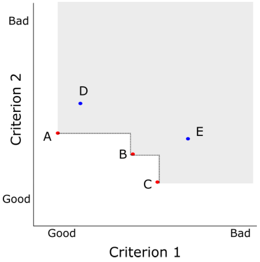
This paper instead presents the dominance approach, which does not arbitrarily prioritise criteria or set subjective thresholds. Instead, dominance is used to identify all the parameter sets that are on the Pareto efficient frontier. These are the parameter sets that are objectively best, where an improvement in one criterion can only be made by reducing the fit for another criterion (see Figure 1). While this approach is well established in operations research for multi-criteria decision making or optimisation (Müssel et al. 2012), it is less well known in social simulation (with some exceptions, such as Schmitt et al. 2015).
The method is described using a case study: calibrating the TELL ME model concerning protective behaviour in response to an influenza epidemic. This paper first presents the model structure and the parameters required to operationalise the links between attitude, behaviour and epidemic spread. The description focuses on the necessary background to understand the calibration process presented in the following sections. The approach to setting parameter values is then described, with the results of that process and conclusions following.
Case study description: TELL ME Model
The European funded TELL ME project[1] concerned communication before, during and after an influenza pandemic. Ending in January 2015, it was intended to assist health agencies to develop communication plans that encourage people to adopt appropriate behaviour to reduce influenza transmission. One project output was a prototype ABM, to explore the potential of such models to assist communication planning. The agents in that model represent people making decisions about protective behaviour (such as vaccination or hand hygiene) in light of personal attitudes, norms and epidemic risk.
The core of the TELL ME model is individual agents making decisions about whether to adopt behaviour to reduce their chance of becoming infected with influenza. Protective behaviour is adopted (or dropped) by an agent if the weighted average of attitude, subjective norms and perception of threat exceeds (or falls below) some threshold.
Each agent is attached to a patch (a location defined by a grid) overlaid on a map of the country in which the epidemic is being simulated. The epidemic is mathematically modelled by the patches; there is no transmission between individual agents. The infectivity at any patch is adjusted for the proportion of local agents who have adopted protective behaviour and the efficacy of that behaviour. In addition, the number of new infections in nearby patches is a key input to each agent's perception of threat. Thus, the agent protective behaviour decisions and the transmission of the epidemic are mutually dependent.
The operationalisation of this model design is described briefly below. This description focuses on those elements of the model that were calibrated using dominance. The behaviour of the agents is also affected by communication plans, which are input to the model as sets of messages. The communication elements were disabled for calibration purposes due to lack of data, and are therefore not described here. The model was implemented in NetLogo (Wilensky 1999), with the full code, complete model design (Badham and Gilbert 2015) and other documentation available online[2].
Epidemic transmission
The epidemic is modelled by updating counts for each disease state of the population at each patch. For influenza, a suitable epidemic model is the SEIR model, in which people conceptually start in the susceptible (S) state, become exposed (E) but not yet infectious, then become infectious (I) and are eventually removed from calculations (R) because they either recover and become immune or they die. The model represents this process mathematically (Diekmann et al. 2000), governed by transition rate parameters ( \(\beta\) for \( S \rightarrow E\) , \( \lambda\) for \( E \rightarrow I\) , and \( \gamma\) for \( I \rightarrow R\) ).
| $$ \begin{aligned} \frac{dS}{dt} &= -\beta SI \\ \frac{dE}{dt} &= \beta SI - \lambda E \\ \frac{dI}{dt} &= \lambda E - \gamma I \\ \frac{dR}{dt} &= \gamma I \\ \end{aligned} $$ | (1) |
In each patch or region (\( r\) ), the value of the transition rate parameter from S to E ( \( \beta\) ) is reduced in accordance with the behaviour decisions taken by individuals at that patch and the efficacy ( \( E\) ) of the behaviour. The reduced infectivity rate (calculated with equation 2) is used in the transmission equations (equation 1), leading to a lower local incidence. To support a mix of behaviour (and hence different reductions in infectivity between patches), each patch is home to at least ten agents, with greater numbers in those patches that correspond to high population density real world locations.
| $$ \beta_r = \beta \left( 1 - P_r E \right) $$ | (2) |
To allow the epidemic to spread, a proportion of estimated new exposures for a region is actually created in neighbouring patches to simulate travel. This requires two additional parameters, the proportion of new infections created at other locations, and the split between neighbouring or longer distance patches.
Operationalising decisions about protective behavior
The agents' behaviour decisions are based on three psychological models: the Theory of Planned Behavior (Ajzen 1991), Health Belief Model (Rosenstock 1974), and Protection Motivation Theory (Maddux et al. 1983). The key factors of attitude, norms and threat from these models were used as the inputs for agent behaviour. The agent compares the weighted average of the three inputs to a threshold (equation 3) for each type of behaviour (vaccination or other protective). If the value is higher, the agent adopts the non-vaccination behaviour or seeks vaccination, and non-vaccination behaviour ceases once the value falls below the relevant threshold. Vaccination cannot be dropped. Threat has the same value for both types of behaviour, but attitude, norms, weights and thresholds may be different.
| $$ \begin{aligned} {\omega_A A + \omega_N N + (1 - \omega_A - \omega_N) T_t \ge B} \quad \text{adopt behavior} \\ {\omega_A A + \omega_N N + (1 - \omega_A - \omega_N) T_t < B} \quad \text{abandon behavior} \\ \end{aligned} $$ | (3) |
Attitude is operationalised as a value in the range [0,1], initially selected from a distribution that reflects the broad attitude range of the population. Subjective norms describe how a person believes family, friends and other personally significant people expect them to behave and the extent to which they feel compelled to conform. The norm is operationalised as the proportion of nearby agents who have adopted the behaviour.
Perceived threat (\(T_t\)) reflects both susceptibility and severity (equation 4). Following the method of Durham and Casman (2012), susceptibility is modelled with a discounted (\( \delta\) ) cumulative incidence time series. This means that perceived susceptibility will increase as the epidemic spreads but recent new cases (\( c_t\) ) will impact more strongly than older cases. In contrast to the cited paper, only nearby cases are included in the time series for the TELL ME model, so perceived susceptibility will be higher for the simulated individuals that are close to the new cases than for those further away. Severity is included as a simple ‘worry' multiplier (\(W\) ), and can be interpreted as subjective severity relative to some reference epidemic.
| $$ \begin{aligned} s_t &= \delta s_{t - 1} + c_{t - 1} \\ T_t &= W s_t \\ \end{aligned} $$ | (4) |
Calibration Process
From the model structure discussion, it is clear that there are many parameters to be determined. Some may be estimated directly from measurable values in the real world, such as population counts. Ideally, unmeasurable values should be calibrated to optimise some measure of goodness of fit between model results and real world data.
The first phase simplified the model to reduce the number of parameters influencing results. This was done by excluding the communication component and fixing protective behaviour to have no effect. Other values were fixed at values drawn from literature, specifically those that affected the distribution of attitudes and the transmission of the epidemic. The exclusion of some components and setting of other parameters to fixed estimates can be interpreted as reduction in the dimensions of the parameter space, reducing the scope of the calibration task.
The second phase calibrated the parameters that are central to the model results; those that govern the agents' decisions to adopt or drop protective behaviour as an epidemic progresses (weights in equation 3 and discount in equation 4). This phase is where dominance was used, to assess parameter sets against three criteria: size and timing of maximum behaviour adoption, as well as the more usual criterion of minimising mean squared error between actual and estimated behaviour.
The model parameters are summarised in Table 1, together with how they were used in the calibration process. While the TELL ME model included both vaccination and non-vaccination behaviour, only the latter is reported here because the process was identical. Non-vaccination behaviour was calibrated with various datasets collected during the 2009 H1N1 epidemic in Hong Kong. The calibration process is described in more detail in the remainder of this section.
| Symbol | Description | Value |
| \(A_0\) | Base attitudes | distribution |
| \(P_r\) | Population by region | GIS data |
| \(R_0\) | Basic reproduction ratio (gives \(\beta\)) | Fixed at 1.5 |
| \(\frac{1}{\lambda}\) | Latency period \(E \rightarrow I\) | Fixed at 2 |
| \(\frac{1}{\gamma}\) | Recovery period \(I \rightarrow R\) | Fixed at 6 |
| Population traveling | Fixed at 0.30 | |
| Long distance traveling | Fixed at 0.85 | |
| \(W\) | Severity relative to H1N1 | Fixed at 1 |
| \(\delta\) | Incidence discount | To be calibrated |
| \(\omega_A\) | Attitude weight (x2) | To be calibrated |
| \(\omega_N\) | Norms weight (x2) | To be calibrated |
| \(B\) | behavior threshold (x2) | To be calibrated |
| \(E\) | behavior efficacy (x2) | Fixed at 0 |
| Meaning of 'nearby' | Fixed at 3 patches |
Dimension reduction: protective behaviour
Attitude distribution was based on a study of behaviour during the 2009 H1N1 epidemic in Hong Kong (Cowling et al. 2010), which included four questions about hand hygiene: covering mouth when coughing or sneezing, washing hands, using liquid soap, and avoiding directly touching common objects such as door knobs. A triangular distribution over the interval [0,1] with mode of 0.75 was used to allocate attitude scores in the model as an approximation to these data.
The efficacy of protective behaviour (\( E\) ) was set to zero (ineffective) during calibration. That is, agents respond to the changing epidemic situation in their decision processes, but do not influence that epidemic. This ensures simulations using the same random seeds will generate an identical epidemic regardless of behaviour adoption, allowing simulated behaviour to respond to the relevant incidence levels.
Dimension reduction: epidemic transmission
Several parameters that influence epidemic spread were estimated from data. These are the various transition rates between epidemic states, the structure of the population in which the epidemic is occurring, and the mobility of that population. The multiplier in equation (4) was set at \( W=1\) , establishing H1N1 as the reference epidemic.
The basic reproductive ratio (denoted \(R_0\) ) is related to the parameters in equation (1) with \( R_0 = \frac{\beta}{\gamma}\) (Diekmann et al. 2000). \(R_0\) for the 2009 H1N1 epidemic was estimated as 1.1-1.4 (European Centre for Disease Prevention and Control 2010). Calibration experiments were run with \( R_0 = 1.5\) (the lowest value for which an epidemic could be reliably initiated), latency period of 2 days (European Centre for Disease Prevention and Control 2010), and infectious period of 6 days (Fielding et al. 2014) .
The population at each patch was calculated from population densities taken from GIS datasets of projected population density for 2015 (obtained from Population Density Grid Future collection held by Center for International Earth Science Information Network - CIESIN - Columbia University & Centro Internacional de Agricultura Tropical- CIAT 2013). These densities were adjusted to match the raster resolution to the NetLogo patch size and then total population normalised to the forecast national population for 2015 (United Nations, Department of Economic and Social Affairs, Population Division 2013).
As epidemic processes (equation 1) occur independently within each patch, the model explicitly allocates a proportion of the new infections created by a patch to other patches to represent spreading of the epidemic due to travel. The proportion of new infections allocated to other patches was set at 0.3, with 0.85 allocated to immediate neighbours and 0.15 allocated randomly to patches weighted by population counts. These values provide a qualitatively reasonable pattern of epidemic spread.
Dominance analysis of behaviour parameters
Four parameters are directly involved in agent adoption of protective behaviour: weights for attitude and norms, the discount applied for the cumulative incidence, and the threshold score for adoption (\( \omega_A\), \(\omega_N\), \(\delta\), and \( B\) in equations 3 and 4). Briefly, multiple simulations were run while systematically varying these parameters to generate a behaviour adoption curve. That curve was assessed against empirical data on three criteria, and dominance analysis was used to identify the best fit candidates.
Broadly, the empirical behaviour data has an initial population proportion of approximately 65%, which rises to 70% and then falls below the starting level. This rise and fall was considered the key qualitative feature of the data and two aspects were included: timing and size of the bump. The three criteria to select the best fit parameter sets were:
- mean squared error between prediction and actual over all points in the data series (MSE);
- the difference in values between the maximum predicted adoption proportion and maximum actual adoption proportion (\(\Delta\) Max); and
- the number of ticks (days) between the timing of the maximum predicted adoption and maximum actual adoption (\(\Delta\) When).
Experiments and dominance analysis were performed with the Sandtable Model Foundry (Sandtable 2015). This proprietary system was used to manage several aspects of the simulation in a single pass: sampling the parameter space, submitting the simulations in a distributed computing environment via the NetLogo API, comparing the result to the specified criteria, and calculating the dominance fronts. As each run takes several minutes, the sampling and distributed computing environment made it feasible to comprehensively explore the parameter space in a reasonable time and the within-system dominance calculation simplified analysis[3] .
Simulations were run with parameter values selected from the ranges at Table 2, chosen so as to require a contribution by attitude (\(\omega_A \ge 0.2\)) to support heterogeneity of behaviour between agents on a single patch. Parameter combinations were excluded if they did not include contributions by all three influencing factors of attitude, norms (\(\omega_N \ge 0.1\)), and threat (\(\omega_A + \omega_N \le 0.9\)). The parameter space was sampled using the Latin Hypercube method, with 813 combinations selected.
| Parameter | Range |
| Attitude weight \(\omega_A\) | 0.2 by 0.05 to 0.7 |
| Norms weight \(\omega_N\) | 0.1 by 0.05 to 0.5 |
| Incidence discount \(\delta\) | 0.02 by 0.02 to 0.2 |
| Behaviour threshold \(\beta\) | 0.2 by 0.05 to 0.7 |
Ten simulations were run for each parameter combination. Preliminary testing with 30 repetitions indicated that simulations using the same parameters could generate epidemics that differ substantially on when they ‘take off', but they had similar shapes once started, and hence similar behaviour adoption curves (not specifically shown, but visible in Figure 5). Ten of the seeds were retained for use with the calibration simulations. These random seeds generated epidemics with known peaks regardless of the behaviour parameter combination as the generated epidemic was not affected by protective behaviour (since efficacy is set to 0).
The behaviour curves from the 10 simulations were centred on the timestep of the epidemic peak and averaged. The average curve was compared to the (centred) 13 data points of the Hong Kong hand washing dataset (Cowling et al. 2010, supplementary information), for calculation of the three fit criteria.
Parallel plot analysis was used as an exploratory tool. This is an interactive technique using parallel coordinates (Inselberg 1997; Chang 2015) to simultaneously show the full set of model parameters and the criteria metrics. That is, simulation runs can be filtered with specific values or ranges of one or more of the input parameters or difference from criteria.
Dominance analysis was used to identify the best fit candidate parameter sets. This technique assigns each parameter set to a dominance front (using the algorithm of Deb 2002). Front 0 is the Pareto efficient frontier, where any improvement in the fit for one criterion would decrease the fit against at least one of the other criteria (Figure 1). Front 1 would be the Pareto efficient frontier if all the front 0 parameter sets were removed from the comparison, and so on for higher front values until all parameter sets are allocated a front number.
Results
The parameter sets that are not dominated are those on the Pareto efficient frontier (front 0). These are described at Table 3 with their performance against the three criteria. By definition, for all other parameter sets, there is at least one on the frontier that is a better fit on at least one criterion and at least as good a fit on all others. Thus, these are the objectively best candidates.
The choice between these for the best fit overall is subjective, trading performance in one criterion against performance in the others and also adding other factors not captured in the criteria. Two methods were used to assist with that choice, quantitative distance from best fit criteria and qualitative fit of behaviour curves.
| Parameter values | Criteria | ||||||
| Set | \( \Omega_A\) | \(\Omega_N\) | \( \delta \) | \( B \) | MSE | \( \Delta \) Max | \( \Delta \) When |
| 1 | 0.7 | 0.2 | 0.18 | 0.5 | 0 | 0.09 | 78 |
| 2 | 0.7 | 0.2 | 0.1 | 0.5 | 0 | 0.08 | 78 |
| 3 | 0.65 | 0.1 | 0.2 | 0.4 | 0 | 0.05 | 71 |
| 4 | 0.6 | 0.2 | 0.06 | 0.45 | 0 | 0.05 | 84 |
| 5 | 0.55 | 0.1 | 0.1 | 0.35 | 0 | 0.01 | 76 |
| 6 | 0.35 | 0.1 | 0.18 | 0.25 | 0.01 | 0.01 | 73 |
| 7 | 0.65 | 0.1 | 0 | 0.5 | 0.07 | 0.01 | 206 |
| 8 | 0.55 | 0.1 | 0.18 | 0.25 | 0.08 | 0.19 | 69 |
| 9 | 0.7 | 0.2 | 0.14 | 0.3 | 0.12 | 0.26 | 62 |
| 10 | 0.55 | 0.35 | 0.16 | 0.4 | 0.13 | 0.27 | 61 |
| 11 | 0.2 | 0.3 | 0.04 | 0.2 | 0.19 | 0.29 | 36 |
| 12 | 0.3 | 0.35 | 0 | 0.3 | 0.19 | 0.29 | 19 |
| 13 | 0.25 | 0.3 | 0.1 | 0.25 | 0.23 | 0.29 | 9 |
| 14 | 0.25 | 0.5 | 0.14 | 0.25 | 0.29 | 0.29 | 33 |
| 15 | 0.25 | 0.25 | 0.02 | 0.35 | 0.34 | 0.01 | 104 |
The fit for all tested parameter sets is displayed at Figure 2, with the non-dominated (front 0) candidates marked in red and labelled with the set number from Table 3. Each appears in the lower left corner of at least one of the sub-figures. From (a) and (b), a small error in the timing of the maximum adoption cannot be combined with a small error in either of the other properties. Focusing only on those other properties (sub-figure (d), the relevant section of (c) expanded), parameter sets 5 and 6 achieve a much closer maximum adoption compared to sets 3 and 4, with only a small loss in the mean squared error. While the same analysis could have been performed by examining Table 3 directly, the visualisation allows fast comparison, even with a larger number of criteria.

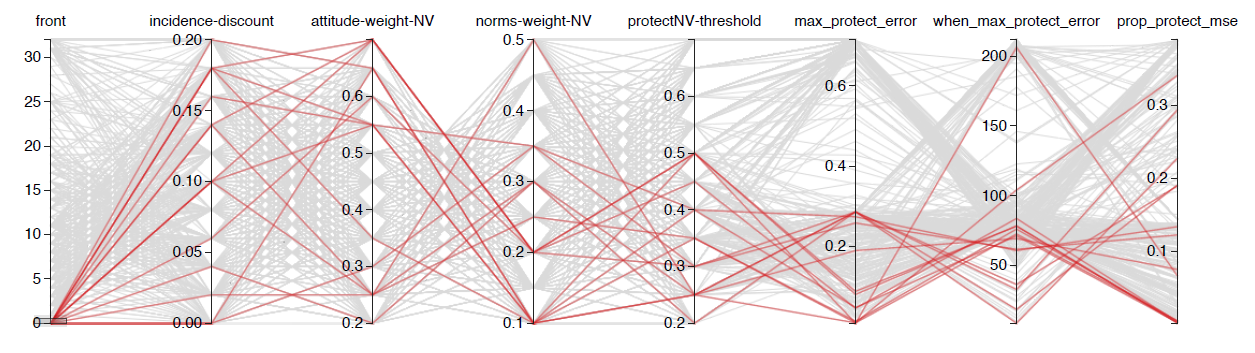
These best fit candidates are also coloured red in the parallel coordinate analysis (see Figure 3). This revealed that good fit parameter sets existed throughout the tested parameter space for the weights and discount, but that the threshold should not exceed 0.5. The main benefit of this analysis, however, is interactive. For example, it can provide a visual method of pattern-oriented modelling filtering, by adjusting ranges on the criteria results and displaying the parameter values of the simulations that survive.
For the qualitative visualisation, fifty simulations were run using the NetLogo BehaviorSpace tool (Wilensky 1999) for each of the non-dominated parameter sets. The average adoption curve is shown in Figure 4. Only sets 1 to 6 display the appropriate pattern of behaviour, with approximately two thirds of the population adopting the behaviour before the start of the epidemic followed by an increase and then return to a similar level once the epidemic has passed. An inspection of Table 3 shows that the mean squared error is similar for all six, but parameter sets 5 and 6 also have a good match in the estimated maximum adoption level, supporting the selection of either of these as the best fit.
Ultimately, parameter set 6 was selected as the best fit and used as the TELL ME non-vaccination behaviour default values. The individual runs for the model with these default parameter values are shown in Figure 5, together with the average behaviour curve.


Discussion
This paper describes a detailed calibration process using the prototype TELL ME model as a case study. The model is complicated, with many components and parameters to reflect policy makers' understanding of their planning environment. It is also complex, with model behaviour shaped by two types of interactions. Personal decisions about protective behaviour affect epidemic progress, which influences perceptions of threat and hence personal decisions. Behaviour decisions of agents are also directly influenced by the decisions of nearby agents, through their perception of norms.
The calibration process first reduced the dimensions of the parameter space by setting epidemic parameters, population density and attitude distribution to values drawn from the literature. Some other parameters were set to values that removed their influence in the model (notably behaviour efficacy and those associated with communication).
This reduced the parameters required to calibrate the model to only four: attitude weight, norms weight, incidence discount and adoption threshold. These parameters control the central process of the model - adoption of protective behaviour in response to an epidemic. With only limited empirical information about behaviour throughout an epidemic, we used pattern-oriented modelling and attempted to calibrate against three weak signals: timing of the behaviour peak (compared to the epidemic peak), maximum level of protective behaviour, and minimising the mean square difference between the simulation estimate and measured behaviour level.
Having three assessment criteria opens the question as to how to compare the runs where they have different rankings across criteria. The standard approach is to set acceptance thresholds for each criterion (Railsback and Grimm 2012) and then select from only those that pass all. However, this is inefficient: if thresholds are set low enough to pass simulations that are generally excellent but are slightly less fit on one criterion, then the thresholds also allow through any simulation that is slightly less fit on all criteria. Instead, we have used the concept of dominance to identify the objectively best parameter sets; for any excluded simulation, there is at least one member of the dominant candidates that is better on at least one criterion and no worse on all others. Additional criteria were used to choose between these objectively good candidates, determining what to give up in order to achieve the best overall fit.
There is little similarity in the non-dominated parameter sets. Very different parameters can achieve similar outcomes (for example, sets 5 and 6), and parameter values in the best fit sets covered a broad range of values. This reflects the interdependence between the parameters and emphasises the difficulties in calibrating the TELL ME model, it would not have been possible to identify these candidates by tuning parameters individually.
The rigorous calibration process was instrumental in detecting structural problems with the model. In particular, the prototype was unable to generate results with a behaviour peak earlier than the epidemic peak, in conflict with the empirical results for hand hygiene during the Hong Kong 2009 H1N1 epidemic. A reasonable fit could have been achieved against a minimum mean squared error single criterion, but assessing against multiple criteria highlighted the timing weakness.
Further consideration of the model rules makes it clear that this is a structural or theoretical gap rather than a failure in calibration. As attitude, weights and the threshold are fixed, change in behaviour arises from changes in the norms or perceived threat. The attitude weight is instrumental in setting the proportion adopted in the absence of an epidemic, but plays no part in behaviour change as the attitudes of agents are constant. As the epidemic nears an agent, incidence increases near the agent, which also increases perceived threat and may trigger adoption. This may also trigger a cascade through the norms (proportion of visible agents who are protecting themselves) component. However, the threat component of the behaviour decision (equation 3) can only respond to an epidemic, not anticipate it, and the norms component can only accelerate adoption or delay abandoning it. Therefore, regardless of parameter values, the simulation is unable to generate a pattern with a behaviour curve peak before the epidemic peak.
Conclusion
Ultimately, the TELL ME ABM was unable to be calibrated adequately for policy assessment. That is, the best fit parameter set was used as the model default values, but the simulation did not produce realistic model behaviour. For the purposes of the TELL ME project, this outcome was disappointing but not unexpected. The ABM was a prototype intended to identify the extent to which such a model could be developed for planning purposes. The attempt highlighted both the limited empirical information about behaviour during an epidemic and the absence of information about the effect of communication. Relevant behavioural information must be collected if a full planning model is to be developed in the future.
In contrast, the use of dominance was successful in identifying candidate parameter sets that are objectively best against several competing criteria. Selection between these candidates was then relatively simple as only a limited number needed to be considered. Further, the rigorous process highlighted structural problems in the model as the desired timing of the behaviour peak could not be achieved while also achieving good performance in other criteria.
Acknowledgements
This paper benefited enormously from thoughtful comments and questions from several referees, and the authors would like to thank them for their care and effort. We would also like to thank Nigel Gilbert, Andrew Skates and other colleagues at the Centre for Research in Social Simulation (University of Surrey), and at Sandtable, and the TELL ME project partners for their input into the development of the TELL ME model.Notes
- This research has received funding from the European Research Council under the European Union’s Seventh Framework Programme(FP/2007-2013), Grant Agreement number 278723. The full project title is TELL ME: Transparent communication in Epidemics: Learning Lessons from experience, delivering effective Messages, providing Evidence, with details at http://tellmeproject.eu/
- The model and users' guide are also lodged with OpenABM . The model and users' guide are also available from the CRESS website as is the working paper with the detailed technical information. The calibration simulation dataset is available on request from the first author.
- Similar functionality could be achieved within an open source environment by combining tools: one for the parameter space sampling and simulation management (such as OpenMOLE, MEME or the lhs and RNetLogo packages in R), and another to analyse the results and calculate the dominance fronts (such as the tunePareto package in R).
References
AJZEN, I. (1991). The theory of planned behavior. Organizational Behavior and Human Decision Processes, 50(2), 179-211. [doi:10.1016/0749-5978(91)90020-T]
BADHAM, J. M. & Gilbert, N. (2015). TELL ME design: Protective behaviour during an epidemic. CRESS Working Paper 2015:2, Centre for Research in Social Simulation, University of Surrey.
CENTER for International Earth Science Information Network - CIESIN - Columbia University & Centro Interna- cional de Agricultura Tropical - CIAT (2013). Gridded population of the world, version 3 (GPWv3): Population density grid, future estimates (2015): http://sedac.ciesin.columbia.edu/data/set/gpw-v3-population-density-future-estimates.
CHANG, K. (2015). Parallel Coordinates v0.5.0. Available from https://syntagmatic.github.io/parallel-coordinates/.
COWLING, B. J., Ng, D. M., Ip, D. K., Liao, Q., Lam, W. W., Wu, J. T., Lau, J. T., Griffiths, S. M. & Fielding, R. (2010). Community psychological and behavioral responses through the first wave of the 2009 influenza A (H1N1) pandemic in Hong Kong. Journal of Infectious Diseases, 202(6), 867-876. [doi:10.1086/655811]
DEB, K., Pratap, A., Agarwal, S. & Meyarivan, T. (2002). A fast and elitist multiobjective genetic algorithm: Nsga-ii. Evolutionary Computation, IEEE Transactions on, 6(2), 182-197.
DIEKMANN, O. & Heesterbeek, J. (2000). Mathematical Epidemiology of Infectious Diseases. Wiley Chichester.
DURHAM, D. P. & Casman, E. A. (2012). Incorporating individual health-protective decisions into disease trans¬mission models: a mathematical framework. Journal of The Royal Society Interface, 9(68), 562-570.
EUROPEAN Centre for Disease Prevention and Control (2010). The 2009 A(H1N1) pandemic in Europe. Tech. rep., ECDC, Stockholm.
FIELDING, J. E., Kelly, H. A., Mercer, G. N. & Glass, K. (2014). Systematic review of influenza A(H1N1)pdm09 virus shedding: duration is affected by severity, but not age. Influenza and Other Respiratory Viruses, 8(2), 142-150.
INSELBERG, A. (1997). Multidimensional detective. In Information Visualization, 1997. Proceedings, IEEE Symposium on, (pp. 100-107). IEEE. [doi:10.1109/infvis.1997.636793]
MADDUX, J. E. & Rogers, R. W. (1983). Protection motivation and self-efficacy: A revised theory of fear appeals and attitude change. Journal of Experimental Social Psychology, 19(5), 469 - 479.
MOSS, S. (2007). Alternative approaches to the empirical validation of agent-based models. Journal of Artificial Societies and Social Simulation, 11 (1), 5: https://www.jasss.org/11/1/5.html.
MUSSEL, C., Lausser, L., Maucher, M. & Kestler, H. A. (2012). Multi-objective parameter selection for classifiers. Journal of Statistical Software, 46(5).
RAILSBACK, S. F. & Grimm, V. (2012). Agent-based and individual-based modeling: a practical introduction. Princeton University Press.
ROSENSTOCK, I. M. (1974). The health belief model and preventive health behavior. Health Education & Behavior, 2(4), 354-386.
SANDTABLE (2015). White paper: The sandtable model foundry: http://www.sandtable.com/wp-content/uploads/2015/06/sandtable_model_foundry_wp_6_2.pdf.
SCHMITT, C., Rey-Coyrehourcq, S., Reuillon, R. & Pumain, D. (2015). Half a billion simulations: evolutionary al¬gorithms and distributed computing for calibrating the simpoplocal geographical model. Environment and Planning B, 42(2), 300-315.
UNITED Nations, Department of Economic and Social Affairs, Population Division (2013). World population prospects: The 2012 revision (total population, 2015, medium variant): http://data.un.org/.
WIEGAND, T., Revilla, E. & Knauer, F. (2004). Dealing with uncertainty in spatially explicit population models. Biodiversity & Conservation, 73(1), 53-78.
WILENSKY, U. (1999). Netlogo. Available from http://data.un.org/http://ccl.northwestern.edu/netlogo/.