
Introduction
This paper is intended to show the similarities between simulation modelling in general and a method of formalising theories, which was developed some thirty years ago (Sneed 1979; Balzer et al. 1987) and has been used to reconstruct theories in sciences such as physics, but only rarely in sciences such as psychology (Westmeyer 1992), economics (Stegmüller et al. 1981; Alparslan & Zelewski 2004), sociology and political science (Druwe 1985; Troitzsch 1987, 2012b). Only in a few cases has the analogy between the 'non-statement view' of reconstructing and formalising theories and the simulation of theory-derived models been shown: In sciences such as physics, this is not necessary as many dynamic phenomena can be described with classical mathematics, such as systems of ordinary, partial or stochastic differential equations, which lend themselves to a reformulation in terms of this philosophy of science approach (to be described in Section 2.7). This also holds for the neoclassic methodology in economics. However, in many cases where emergent phenomena on a macro level resulting from interactions between elements of a micro level need to be described, even stochastic differential equations might not be sufficient to explain the emergent phenomena. This is particularly the case when the elements of the micro level are inhomogeneous, which is typical in systems which economics, sociology and political science are interested in. Where the elements of social systems can be simplified as consisting of homogeneous elements, an approach with stochastic differential equations is sometimes sufficient, as has been shown by Weidlich & Haag (1983), Helbing (1991/92) and, more recently, by Johansson et al. (2008) (for a more detailed discussion see Troitzsch (2009, 2012a). In the case of social science research that looks at systems of inhomogeneous, interacting and interpreting human actors, only few papers have discussed the analogy between simulation and 'non-statement view' reconstruction (Troitzsch 1992, 1994, 2012b; Balzer & Moulines 2015).
The paper is structured as follows. In the next section, the use of the terms ‘axiom’ and ‘axiomatisation’ will be discussed, and a short description of theory reconstruction according to the ‘non-statement view’ will be given. Section 3 will exemplify this reconstruction process with the famous segregation model of Schelling (1971) while Sections 4 and 5 will apply this formalisation method to an extension of Schelling’s model with structural inhomogeneity and behaviour rules that change over time. It is worth noting that in these cases changes on the macro level in turn change due to the individual changes, as described with the 'boat' or 'bath-tub' metaphor first coined by Coleman (1990, p. 8). Finally, Section 6 tries to assess the advantages of the 'non-statement view' for computational social science at large against a slightly less formal agent-based simulation approach.
Axioms and axiomatisation of a theory
Axioms in the social sciences
The word 'axiom' seems to have been used for the first time in the context of Euclid’s geometry where it is understood as a statement which need not and cannot be proven as "an established principle or a self-evident truth" (Merriam-Webster, "axiom") or a "maxim, that has found general acceptance or is thought worthy of common acceptance whether by virtue of a claim to intrinsic merit or on the basis of an appeal to self-evidence" (Encyclopædia Britannica 2014, “axiom”).
In a talk given in June 1971, Suppes (1974, p. 472), after having talked mainly about axiomatisation approaches in physics, stated:
Many problems of interest in the behavioral and social sciences have also been treated from an axiomatic standpoint. Much of the contemporary work in mathematical economics satisfies a high standard of axiomatization, and when not explicitly so stated, it can easily be put within a standard set-theoretical framework without difficulty. On the other hand, with the exception of some of the problems of measurement I mentioned earlier, the impact of the theory of models as developed in logic and the kind metamathematical questions characteristic of that theory have not been widely applied in the social sciences, and the relation of these sciences to fundamental questions of logic has not had the history of examination characteristic of problems of long standing in physics.
In what followed in his talk, he gave an example of an axiomatisation of stimulus-response theory inspired by previous work (Suppes 1969) and mentioned a number of similar attempts mainly in equilibrium economics — which is favoured thanks to its high level of mathematisation. This is also why one of the early top Russian readers in mathematics named only "political economy" as a social science subdiscipline apt for mathematisation and axiomatisation:
Of course, in the study of such complicated phenomena as occur in biology and sociology, the mathematical method cannot play the same role as, let us say, in physics. In all cases, but especially where the phenomena are most complicated, we must bear in mind, if we are not to lose our way in meaningless play with formulas, that the application of mathematics is significant only if the concrete phenomena have already been made the subject of a profound theory. In one way or another, mathematics is applied in almost every science, from mechanics to political economy (Aleksandrov 1999, p. 4).
One must, however, admit that (nearly) all those axiomatisations of theories in the social sciences at large were applied to cases where either only the macro level was considered (in economics) or where only the micro level (psychology and sociology of small groups) was considered. Indeed, the problem of the interaction between these two (and potentially even more) levels was only very rarely the object of axiomatisation attempts — at least before the era of agent-based modelling and its predecessors in multilevel modelling. Economics used as "one of the best examples [...] the systems of equations of the mathematical theory of prices [...] to describe the general character of the order that will form itself" (Hayek 1967, p. 261) whereas sociology often used game theory as in Coleman’s reconstruction of an experiment conducted by Mintz (1951) (Coleman 1990, p. 203–215), to name just two extreme examples.
In the context of this paper, we use the word 'axiom' in the sense of a "condition [...] that ha[s] to be satisfied by the basic notions of the theory in question” (Balzer et al. 1987, p. 24), such that it is not a statement that is held to be true but the predicate that the theory makes about its intended applications
The 'non-statement view' and simulation
To introduce the procedures of reconstructing a theory along the lines of the 'non-statement' view ("reconstruction procedures", Balzer et al. 1987, p. 23)[1], we use a very simple theory from classical mechanics, namely Hooke’s early theory of elasticity — Petroski (1996, p. 9–11) tells the story of Hooke’s discovery — which says "that up to a limit, each object stretches in proportion to the force applied to it". Hooke’s experiment consists of a spring whose upper end is fixed and whose lower end can be loaded with one or more small weights which will extend the spring by a measurable amount. The law says that (within a certain range) the extension is proportional to the number of the small weights hanging from the spring. Thus, this law can be described with just two terms which are measurable without any knowledge of springs: the number \(N\) of identical weights and the length \(L\) of the extension. Hooke found out that for any spring the two numerical values were proportional with different proportionality factors \(k_s\) for different springs \(s\): \(N=k_s L\) such that this law could be used for weighing things with unknown weights.
A certain Hooke-like experiment can be understood as a model[2] of classical particle mechanics (CPM). In this simplification of the discussion in (Balzer et al. 1987, p. 29–34), it is understood that \(N\) and \(L\) are non-theoretical terms with respect to CPM (or rather: with respect to Hooke’s spring law HSL, as we will call this extremely simplified version from now on), given that counting identical weights and measuring the length of the extension have nothing to do with springs. On the other hand, the ‘device constant’ \(k_s\) for spring s is not even conceivable and hence unmeasurable without using HSL. Thus it has to be considered as a "theoretical term with respect to HSL" as before stating Hooke’s law it is totally unclear whether \(k_s\) also depends on the number of weights \(N\) appended to the spring. In terms of (Balzer et al. 1987) we can now formulate:
Mpp(HSL): \(x\) is a partial potential model of Hooke’s spring law (\(x\) ∈ Mpp(HSL)) iff there exist \(S, W, N, L, k^*\) such that
- \( x = \langle S, W, N, L, k\rangle\)
- \(S\) is a finite set [of springs]
- \(W\) is a finite set [of identical weights]
- \(N: \cal{P} (W) \times S \rightarrow \cal{N}\) [\(N(\bar{w},s)\) yielding the number of identical weights loaded at the lower end of the spring where \(\bar{w}\subset W\) denotes the collection of weights hanging from spring \(s \in S\)]
- \(L: \cal{P} (W) \times S \rightarrow \cal{R}^+\) [\(L(\bar{w},s)\) yielding the length of the extension produced by a subset of identical weights at the lower end of the spring]
- \(k^*: \cal{P} (W) \times S \rightarrow \cal{R}^+\) [\(k^*(\bar{w},s)\) yielding the quotient \(N(\bar{w},s)/L(\bar{w},s)\)].
In this definition, \(k^*\) is not yet a device constant as it does not only depend on the spring but also on the collection of weights hanging from the spring. Only when Hooke detected that at least for small extensions \(k\) only depended on the spring, he could formulate:
Mp(HSL): \(x\) is a potential model of Hooke’s spring law (\(x\) ∈ Mp(HSL)) iff there exist \(S, W, N, L, k\) such that
- \(x = \langle S, W, N, L, k\rangle\)
- \(S\) is a finite set [of springs]
- \(W\) is a finite set [of identical weights]
- \(N: \cal{P} (W) \times S \rightarrow \cal{N}\) [\(N(\bar{w},s\) yielding the number of identical weights loaded at the lower end of the spring]
- \(L: \cal{P} (W) \times S \rightarrow \cal{R}^+\) [\(L(\bar{w},s)\) yielding the length of the extension produced by a subset of identical weights at the lower end of the spring]
- \(k: S \rightarrow \cal{R}^+\) [\(k(s)\) yielding the quotient \(N(\bar{w},s)/L(\bar{w},s)\) where \(\bar{w}\subset W\) denotes the collection of weights hanging from spring \(s \in S\)]
M(HSL): \(x\) is a model of Hooke’s spring law (\(x\) ∈ M(HSL)) iff there exist \(S, W, N, L, k\) such that
- \(x = \langle S, W, N, L, k\rangle\)
- \(x \in \) \(\textbf{M_p(HSL)}\)
- \(\forall \bar{w} \subset W \quad \forall L < L_0\) and \(\forall s \in S\) : \(k(s) = N(\bar{w},s)/L(\bar{w})\) is a constant which does not depend on \(\bar{w}\).
Schelling’s segregation model revisited
Schelling's model reconstructed
The famous Schelling model (Schelling 1971) has been programmed very often but rarely has it been used to analyse the dependency of the segregation index on input parameters such as density, group sizes and threshold (except perhaps when Squazzoni (2012, p. 90–92) compared the similarity index dynamics for three different threshold values denoting the "preference of like neighbors at 25, 33 and 50%" — see also Epstein & Axtell (1996, p. 165–171). Density, for instance, was typically set to 85 per cent (Bruch & Mare 2006, p. 674, footnote 13), and group sizes were typically equal, also in the models using, for instance, three subpopulations (Muldoon et al. 2012, p. 42), but occasionally an "empirical race-ethnic composition" was used (Bruch & Mare 2006, p. 674, footnote 12). Furthermore, it has never been used to analyse the behaviour of the model systematically when the individuals do not have identical thresholds but thresholds following a certain distribution which might also be different between groups (except Gilbert 2002). A mathematical analysis of the Schelling model and some of its possible extension was given by Zhang (2004) who showed that segregation is "stochastically stable" (p. 148).
In this section, an attempt is made to reconstruct Schelling’s model in terms of the “non-statement view” introduced above. The "reconstruction procedure" is quite similar to the one on in Section 2.7.
A run of a Schelling simulation model written in NetLogo (Wilensky 1997) can be understood as a model of Schelling’s segregation theory (SST), where it is understood that in any real-world context:
- the individuals occupying houses or apartments or, more generally, city blocks in their world,
- their density,
- their individual ‘colours’ and
- the segregation index which can be easily calculated from the data defining which city blocks are occupied by which individual agent(s)
Hence, a potential model of SST can be defined as
Mp(SST): \(x\) is a potential model of Hooke’s spring law (\(x\) ∈ Mpp(SST)) iff there exist \({\cal W}, W, P, \ell, T, \theta, b, {\mathbf c}, \phi, \delta, \varsigma\) such that
- \(x = \langle {\cal W}, W, P, \ell, T, \theta, b, {\mathbf c}, \phi, \delta, \varsigma \rangle\)
- \(W\) is a set of pairs \(\langle W, P\rangle\) [each consisting of a city and its inhabitants or, in the simulation model, the ‘world’ of a Netlogo model interface together with the turtles on it];
- \(W\) is a finite set [of city blocks or, in the simulation model, of patches, collecting all city blocks of the target system or, in the simulation model, the ‘world’ of a NetLogo model interface];
- \(P\) is a finite set [of persons or households moving between city blocks or, in the simulation model, of turtles moving between patches];
- \(\ell: P \rightarrow \{ \ell_1, \ell_2 \}\) [\(\ell(p)\)] yielding the feature of a person in question, for instance their language or, in the simulation model, the colour of a turtle];
- \(T\) is a finite set [of points in time when census records are taken or, in the simulation model, of ticks];
- \(\theta: P \times T \rightarrow [0,1]\) [\(\theta(p,t)\) yielding a threshold value helping person or turtle p to decide whether to stay or to move at time t];
- \(b: P \times T \rightarrow W\) [\(b(p,t)\) yielding the city block b where household \(p\) lives at a certain census time \(t\) or, in the simulation model the patch b the turtle p occupies at a certain tick \(t\) of the simulation model];
- \({\mathbf c}: W \rightarrow \{c_{xmin}, ..., c_{xmax}\}\times \{c_{ymin}, ..., c_{ymax}\}\) [\({\mathbf c}(b)\) yielding the integer coordinates of a city block or, in the simulation model, of a patch];
- \(\phi: P \times T \rightarrow [0,1]\) [\(\phi(p,t)\) yielding the proportion of persons of the same colour in the Moore neighboorhood of a certain person at a certain census time or, in the simulation model, the same];
- \(\delta: P \times T \rightarrow W\) [\(\delta(p,t)\) yielding the city block or, in the simulation model, the patch to which person (or turtle) \(p\) will move at time \(t\); \(\phi(p,t)>\theta(p,t)\rightarrow\delta(p,t)=b(p,t), \phi(p,t)\ge\theta(p,t)\rightarrow\delta(p,t)\not=b(p,t)\), i.e. iff the proportion of persons of the same colour in the Moore neighbourhood of \(p\) is below the threshold (\(\theta(p,t)\) this person or turtle will move to the nearest free city block or patch or to a city block or patch where the neighbourhood seems to be more convenient];
- \(\varsigma: {\cal W} \rightarrow [0,1]\) yielding the segregation index for the whole collection of city blocks and their inhabitants or, in the NetLogo model, of the simulated world and its turtles].
The segregation index D mentioned in item 12 is defined (Duncan & Duncan 1955) as
| $$D = \frac{1}{2}\sum_{i=1}^n\left|\frac{x_i}{X} - \frac{y_i}{Y}\right|$$ | (1) |
Some more derived terms used later on need to be mentioned here:
- the minority size \(\nu\) defined as \(\frac{|\{p \in P | \ell(p) = \ell_1\}| }{|P|}\)
- the density \(d\) defined as \(\frac{|P|}{|W|}\)
Intended applications of STT
Some of these terms might not be measurable in intended real-world applications of SST:
- \(\theta\) is quite difficult to measure when asking people for a real number in the interval [0;1] to describe be-yond which percentage of similar neighbours in their vicinity they are happy or below which threshold they would take a certain action. Other sources of information about such propensities — census data or data from registration offices, from which removal frequencies can be obtained — do not yield more reliable information about actual individual propensities. Approaches to overcome this difficulty have been made for instance by da Fonseca Feitosa et al. (2011), Wong (2013) and Benenson et al. (2003). In most simulation models published so far based on SST implementations, \(\theta\) has been a constant for all members of both subpopulations in each simulation run, much like the device constant in HSL, but, see below, this is, of course, not the only possible interpretation of \(\theta\).
- \(\delta\) is also quite difficult to measure — one would have to ask interviewees "where would you want to move in case you find that in your neighbourhood there are too many people speaking another language?", as was done by Xie & Zhou (2012) and in a more sophisticated manner by Bruch & Mare (2006) and Lewis et al. (2011). Such a question, however, contains two hypothetical conditions — which is usually discouraged by textbooks on survey methodology (cf. e.g. Converse & Presser 1986, p. 23). This is why in most "Schelling" simulation models \(\delta\) just points to an arbitrary free patch in the vicinity of the current place although there is a lot of empirical evidence that people choose deliberately where to move, and there exist simulation models like the ones cited above which take this into account.
The function \(p\) can in principle be reconstructed from individual data of subsequent censuses (when individual data are kept between census dates) or from records of resident registration offices (if these exist in the context in question).
Intended applications are usually partial potential models of a theory that do not include terms which are theoretical with respect to the theory in question, and here is where intended applications of SST have serious problems for several reasons:
- If, as is usually the case although not in Schelling’s original paper, the world is understood as a torus, there is no real-world correspondence possible at all, but this restriction can easily be solved. The fact that Schelling’s original and nearly all simulation models describe the world structured as a checkerboard is not so much of a problem as Flache & Hegselmann (2001, 5.1) showed that social dynamics "may be widely robust against changes of the underlying standard assumption of rectangular grids".
- Having only two more or less homogeneous subpopulations which differ in exactly one binary feature is a simplification — Gilbert (2002) has pointed this out and showed a number of relaxations and its consequences — and it will be difficult to find a social system which can be described in so simple terms. However, there are modelling attempts which try to overcome this and other simplifications, too, for instance Muldoon et al. (2012) and Durrett & Zhang (2014) with larger neighbourhoods, Lewis et al. (2011) and Wong (2013) with more than two subpopulations.
- Describing neighbourhoods only one-dimensionally with the proportions of inhabitants belonging to distinguishable subpopulations is obviously inadequate, as there are many other motives to move from one city district to another which were for instance taken into account by da Fonseca Feitosa et al. (2011); for the inclusion of the housing market see Zhang (2004).
The partial potential model of SST and its simulation implementation
Leaving the problems in the two previous paragraphs aside for a while, one can now easily map this description of the potential model of SST on Wilensky’s NetLogo simulation model (Wilensky 1997) and the extension described in this paper — see Tables 1 and 4. The extension described here can be run with exactly the features of Wilensky’s original.
| SST term | NetLogo model component |
|---|---|
| \(\cal W\) | the set of all possible runs of the model |
| \(W\) | the patches in a certain run of the model |
| \(P\) | the turtles in a certain run of the model |
| \(\ell\) | the built-in turtle variable color |
| \(T\) | NetLogo's ticks |
| \(\theta\) | the global variable %-similar-wanted — which shows that in original SST the tolerance level is not an individual variable but a global constant, a re-striction first relaxed in (2002) |
| \(b\) | the NetLogo built-in function patch-here |
| \(\mathbf c\) | NetLogo's built-in turtle variables xcor and ycor |
| \(\delta\) | the value of this function is calculated in the procedure update-turtles in Wilensky’s code (similar-nearby)
|
| \(\varsigma\) | the value of this function is calculated in a few lines in the procedure update-globals added to Wilensky’s code but can also be calculated as a single function |
Neither Schelling’s original paper nor any of the following work yields a closed formula connecting the segregation index \(\varsigma\) to the tolerance threshold \(\theta\) — which so far was mostly assumed to be constant for all agents and at all times, with the exception of Gilbert (2002) — or to the density \(d=|P|/|W| < 1\) (which must be strictly \(<1\) as otherwise unhappy agents have no chance to swerve) or to the fractions of the two groups (usually assumed equal, but it is also — and perhaps even more — interesting to find out how segregation works with respect to a minority; the fractions of the groups can easily be expressed in the terms of Mp(SST). But, multiple runs of the simulation model give an opportunity to derive at least a linear or nonlinear regression equation between the segregation index \(\varsigma\) (certainly a macro variable) and one or more of the other macro or micro variables. \(\theta\) although a constant in the original version of SST, is a feature of the individuals and hence a micro variable. In extended versions, however, building on Gilbert (2002), \(\theta\) will become a function of the macro variables and \(\mu_\theta\) and \(\sigma_\theta\), and the individual \(\theta_{p,t}\) will even change their individual values over time depending on local neighbourhoods.
First results
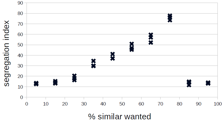
Figure 1 gives a first impression of the dependence of the segregation index on the tolerance threshold: It seems that the dependence is nonlinear — as already observed by Squazzoni (2012, p. 92) — but obviously entirely different for tolerance thresholds below and above 80 per cent. Indeed, above a level of 80 per cent, segregation cannot be achieved as it becomes extremely difficult for the agents to become happy with so strong a demand.
Here, it is important to note that in Wilensky’s implementation account whether these patches meet their needs better than the patches they come from (“keep going until we find an unoccupied patch”; the extended version stops a run when over the last 20 ticks the standard deviation of percent-unhappy was below 1). We will first analyse the results for tolerance levels below 80 per cent in more detail to return to the problem of agents’ unintelligent search for alternative patches.
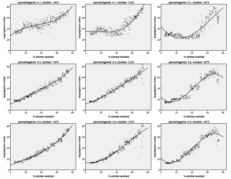
To this end, a Monte Carlo simulation with partly random parameter combinations is run to search the complete parameter space (reasonably leaving out tolerance thresholds above 80 per cent) and to find out how much of the variance of the segregation index can be explained by tolerance threshold (uniformly distributed between 5 and 75 per cent), density (.75,. 85 and .95) and size of the minority group (10, 30, 50 per cent) with 300 runs for each combination of the two latter factors, resulting in 2,700 individual runs. Afterwards, we will extend the model along the lines of the ideas presented by Gilbert (2002).
This yields the scatterplots presented in Figure 2. Note that in these plots only those runs were used where the tolerance threshold did not exceed 65 per cent. Figure 1 shows that the emergent behaviour of the system is different for these high tolerance levels. Most of these graphs show the cubic dependence between tolerance threshold and segregation index.
A first attempt at analysing the outcome of this model is a Monte Carlo simulation with 3,000 runs varying the tolerance threshold, the size of the minority and the density. Here, we want to find out how strong the dependence of the segregation index on these three input parameters is. This analysis shows a variance reduction of nearly 90 per cent (\(R^2=0.872\)). The tolerance threshold is the most important input parameter with a standardised \(\beta= 0.901\), the influence of the minority size is weaker with \(\beta=-0.281\) (the smaller the minority, the higher the segregation index), whereas the influence of the density is not even significant (in spite of the high number of runs, for the relevance or irrelevance of significance in simulation analysis see (Ziliak & McCloskey 2007)) with a standardised \(\beta=-0.028\).
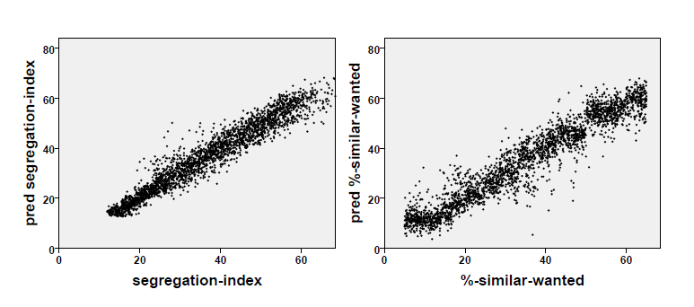
This finding can be generalised to a cubic regression of the segregation index on tolerance threshold \(\theta\), minority size and density \(d\) in this Monte Carlo simulation with 3,000 runs. The variance reduction is slightly higher than in the linear case (\(R^2=0.934\)) and the segregation index can be 'predicted' with a standard error of about 3.66 percentage points. The left-hand diagram of Figure 3 shows how perfect this regression is. However, it is even more interesting for our current concern that the segregation index, the density and the minority size can be used to measure the tolerance threshold[3] — here the variance reduction is also above 90 per cent (\(R^2=0.915\)) and the standard error is about five percentage points (see the right-hand diagram of Figure 3).
This means that SST yields a procedure to measure the value of a term that could not otherwise be measured in real-world scenarios, hence the tolerance threshold is a theoretical variable with respect to SST — much like the case of the device constant of Hooke’s springs which can be measured with HSL. The regression equation can be defined as the axiom of SST stating that the expected value of the tolerance threshold of two homogeneous subpopulations is a cubic function of the three terms specified above and that the parameters of this function are just the 16 regression coefficients (not given here, as it is entirely unclear what the coefficients \(\beta_{111}\) for the product \(\theta \nu d\) or \(\beta_{201}\) for the product \(\theta² d\) mean). So, one could conclude that a "black white segregation index" in New York, Northern New Jersey and Long Island of 81.5, as reported by Frey (2016); Frey & Myers (2005), and the same index for Tucson AZ of 36.9 can be interpreted as a tolerance level (of both subpopulations the same!) of more than 70 and less than 12, respectively.
This said, one must also ask whether this is of any use if we know that Schelling’s model is an idealisation of what can be observed in the real world. We can, of course, extend this model to be at least a little more realistic and make the tolerance threshold a variable that can vary among individuals, between the two subpopulations and, lastly, over time. This is what we will analyse in the next section.
Adding more complexity to Schelling’s model
As already discussed in earlier sections, the version of the model described in the following subsections extends Wilensky’s implementation in several respects. While the extensions above were merely technical (e.g., adding a formula for calculating the segregation index, adding a stopping mechanism when the model run seemed to have stabilised), the extensions dealt with in this section are more substantial and are as follows:
- tolerance related search of a new neighbourhood, i.e. agents do not only search for an unoccupied patch but they look for an unoccupied patch which fits their needs better than the current patch[4];
- tolerance levels can be different for the two subpopulations[5] and , i.e. population
redmight like to live together with populationgreenwhich in turn prefers to live apart fromred— examples are: a rich minority preferring to live in gated communities and a middle class majority taking no offence at rich people living in their neighbourhood or a minority of hooligans who do not care for their neighbourhood but who influence majority people to move away; this leads to \(\theta(p,t)=\theta_i\) iff \(\ell(p)=i\); - tolerance thresholds may differ within each subpopulation (i.e. they have distributions with different statistical parameters, here: means and variances[6]); this means that \(\theta\) is no longer a global constant as in the definition of the potential model of SST, item 7, but instead a random variable approximately normally distributed within each subpopulation \(i\) with mean \(\mu_{\theta,i}\) and standard deviation \(\sigma_{\theta,i}\) censored to the range of [0.05, 0.95];
- tolerance thresholds change over time as a consequence of communication between agents; this means that \(\theta\) is no longer an individual constant but a variable changing over time (see Section 5.1).
Sophisticated search, inhomogeneous and different subpopulations
In a next big Monte Carlo simulation with 6,000 runs, we experiment with the first three extensions listed above. We make a twofold difference:
- one between the simple search of a new place (as coded by Wilensky 1997) and the tolerance related search where the agents look for an unoccupied patch which is at least populated with slightly less agents of the other colour or language — if none is found the agent does not move — and
- between homogeneous subpopulations (all individuals of a subpopulation have the same threshold) and inhomogeneous subpopulations (within each subpopulation the tolerance threshold follows a censored normal distribution with a mean — usually different for the two subpopulations — and a variance of 15 percentage points; censoring makes sure that the individual tolerance threshold remains between five and 95 per cent).
This leads to 1,500 simulation runs for each of the four subexperiments defined by search strategy and subpopulation homogeneity, and in each of the four subexperiments density, minority size and the two means of the tolerance threshold are randomly varied.
The outcome of this experiment is analysed with a linear regression which yields the variance reductions and standardised s collected in Table 2.
| input parameters | simple search | tolerance related search | |||
| homogeneous | inhomogeneous | homogeneous | inhomogeneous | ||
| all | R2 | 0.627 | 0.720 | 0.689 | 0.802 |
| minority size | \(\beta\) | -0.168 | –0.340 | -0.207 | -0.404 |
| density | \(\beta\) | -0.127 | -0.198 | -0.133 | -0.182 |
| tolerance mean minority | \(\beta\) | 0.388 | 0.560 | 0.389 | 0.556 |
| tolerance mean majority | \(\beta\) | 0.670 | 0.533 | 0.696 | 0.513 |
| tolerance means cubic | R2 | 0.757 | 0.649 | 0.748 | 0.647 |
Table 2 shows that the strength of the dependence of the segregation index on the four more or less continuously varied input parameters decreased considerably due to the fact that the two subpopulations now have different tolerance levels — a finding that needs further analysis. On the other hand, it is interesting to see that both internal inhomogeneity and a more sophisticated search strategy increase the strength of the dependence. Here, it is worth noting that at least the former (internal inhomogeneity allows for a more precise prediction or explanation of the segregation index) comes as a surprise and also calls for further analysis. Unlike the case with thresholds identical between the two subpopulations, density now makes a difference, although not a remarkable difference, when thresholds differ between and within subpopulations. Finally, the standardised regression coefficients of the tolerance means are now clearly below the level marked in the previous analysis
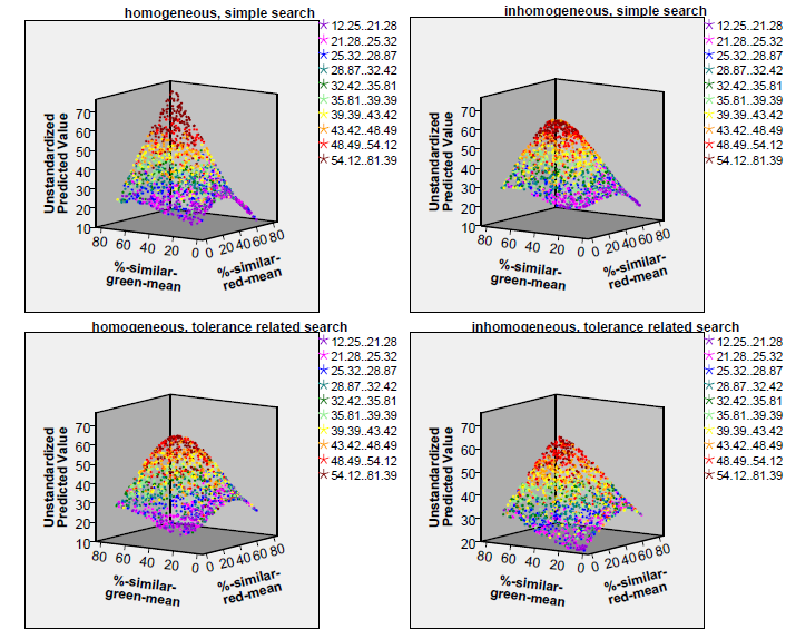
Figure 4 shows how the two tolerance thresholds (or, respectively, their distributions) influence the segregation index. These diagrams show the segregation index values as predicted by a cubic polynomial (its \(R^2\) is also given in Table 2) in the two tolerance means (the coloured dots, however, show the approximate segregation index value as they were yielded by the simulation).
Obviously, it does not matter whether the tolerance threshold distributions of the two subpopulations are different or similar — otherwise the colour shades of the dots in the four diagrams of Figure 4 would have been separated by borders running top down. On the contrary, the colour shades are quite distinctly separated by borders which run parallel to the plane spanned by the two input parameters. Hence, the fiercest segregation occurs when the overall mean tolerance threshold is high: if both subpopulation thresholds are above 50 per cent, a segregation index above 46 can be expected (red and dark red dots in the top far corners of the diagrams) whereas when both are below 30 per cent the expected segregation index will be below 30 (violet, blue and dark green dots in the bottom foregrounds of the diagrams). The overall impression given by the four diagrams does not point to big differences caused by the choice of the two binary input parameters (tolerance level standard deviation 0 vs. 15, simple or tolerance related search strategy). However, perhaps the boundaries between the differently coloured regions of the diagram are less sharp for the diagrams showing homogeneous subpopulations and for the diagrams showing subpopulations applying the simple search strategy (at least this is what one would expect from Table 2). The only remarkable differences between the four diagrams are perhaps the clearer symmetry of the surfaces with respect to the input parameter %-similar-red-mean in the diagrams for homogeneous subpopulations (best visible at the right-hand edge of the surfaces) compared to an asymmetric parabola at the right-hand edges of the diagrams for inhomogeneous subpopulations. Furthermore, it is interesting to see that both the lowest and the highest segregation indices are reached for the simple search in homogeneous subpopulations — as if inhomogeneity and a more sophisticated search strategy lead to a smaller range of the segregation index.
A further extension: Individually different tolerance thresholds changing over time due to communication
The final extension of Schelling’s original model introduces an effect of the experience of agents in their neighbourhoods on their tolerance threshold. The idea behind this extension is that an agent surrounded by a high proportion of agents of the same subpopulation will increase its tolerance threshold, i.e. will want to have an increasing proportion of similar agents around itself, whereas an agent surrounded by a high proportion of agents of the other subpopulation will decrease its tolerance threshold, i.e. will accept an increasing proportion of dissimilar agents around itself. Hence, \(\theta\) is now a function which yields an agent’s individual tolerance threshold as a function of \(\phi\) defined above in the definition of the potential model of SST, item 10, as follows:
| $$\theta(p, t+1) = \theta(p,t) (1 - \varepsilon) + \varepsilon \phi(p,t) $$ | (2) |
The typical outcome of this extended version is also segregation in most cases. This is even more pronounced than in the time-constant versions. However, as can be seen in the two plots at the top right of Figure 4, usually the mean of the distribution of tolerance threshold in the majority subpopulation increases while its variance decreases; for the minority, the opposite holds — this effect is the more graphic the smaller the minority is —, and the most tolerant individuals of each subpopulation can be found at the borders of the clusters.
Another interesting observation is that for the simple search this version of the model produces a never ending wandering of members of one or both subpopulations: Whenever a large proportion of both groups is 'happy', the more tolerant population moves to places where they are not welcome from the point of view of the other population. This leads to an oscillation of the segregation index, of the percentage of similar agents in the neighbourhood and of the percentage of 'unhappy' agents. This is in line with observations made by Weidlich & Haag (1983, p. 86–112) who analysed “the migration of two interacting populations between two parts of a city”, which is certainly an object of analysis that is quite similar to Schelling’s problem, and observed that under certain circumstances, namely one population wanting to live together with the other population and the other population trying to avoid this, the expected or most likely trajectory of the system would become a stable spiral or even a limit cycle. In the current version of the Schelling model, it is usually a spiral — given that the simulation runs are partly stochastic, it is undecidable whether limit cycles really evolve.
Oscillations do not evolve in the case of the tolerance related search discussed above (see 4.1, item 1). Furthermore, they are the more frequent the higher the tolerance means of the two subpopulations are (with both low, no oscillation at all evolves). On the contrary, the segregation stabilises preferably when both initial tolerance levels are low at the same time.
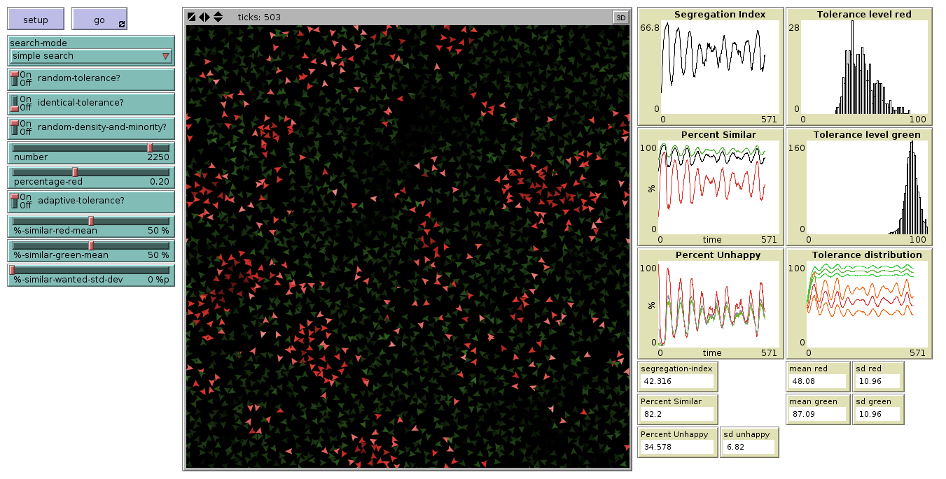
Figure 5 shows the situation of such an oscillating simulation run and the oscillations which could be observed during the run. The simulation started with mean tolerance levels of 63 per cent (in the 11 per cent minority) and 52 per cent (in the 89 per cent majority). From the very beginning, the minority agents were mostly unhappy whereas the majority agents were mostly happy. In the first round, the minority concentrated which made most of them happy. The distribution of their tolerance levels moved down, whereas the distribution of the tolerance levels of the majority moved up and became very narrow. This implies that they tried to move away from the minority agents who, in the meantime, had become more and more friendly towards the majority and followed them which made the majority agents more and more unhappy (and the minority agents as well). Finally, when nearly all minority agents had become unhappy the process repeated.
Real world scenarios of the kind discussed in 5.2–5.4 are difficult to find as longitudinal data for segregation indices are rarely available and usually too short to cover more than one cycle. However, gentrification of a disadvantaged quarter and its later neglect before a new gentrification phase starts is an observation which is more often than not, although unsystematically, made.
| input parameters | tolerance related search | ||
| homogeneous | inhomogeneous | ||
| all | R2 | 0.767 | 0.798 |
| minority size | \(\beta\) | -0.294 | –0.390 |
| density | \(\beta\) | 0.141 | 0.121 |
| tolerance mean minority | \(\beta\) | 0.791 | 0.758 |
| tolerance mean majority | \(\beta\) | 0.247 | 0.225 |
| tolerance means cubic | R2 | 0.716 | 0.683 |
In the remainder of this section, we will only deal with the version where the search for an alternative patch is tolerance related. The linear regression of the segregation index on the same input parameters as above yields the variance reductions and standardised \(\beta\)'s collected in Table 3.
Table 3 shows higher variance reduction than in Table 2. Here, the effect of the tolerance of the majority is considerably reduced, and it seems that the segregation index depends mainly on the initial tolerance level of the minority (which, as in all experiments, ranges between five and 75 per cent).
Finally, the two diagrams in Figure 6 show considerable differences as compared to the two diagrams in the bottom of Figure 4: high initial threshold levels mainly in the minority but also in the majority can lead to much higher segregation indices than in the non-adaptive version. Unlike the non-adaptive version, it is now sufficient for a high segregation index that one of the two subpopulation has a tolerance level distribution with a high mean, and the tolerance level mean of the minority is even more important than the one of the majority.

Conclusions
The paper has shown that the formalism introduced by the ‘non-statement view’ is quite similar to the formalism introduced in simulation models. If one starts with the definition of a potential model of a theory instead with a simulation model (as in the case of a ‘non-statement view’ reconstruction above), the former can be used as a specification of the simulation model before it is written. This can lead to a more straightforward and perhaps to a more transparent simulation program. To show this we refer to another version of the extended Schelling modely[7] which makes the similarity between specification and program much clearer than in the original version of Wilensky (1997). For instance, by comparing Table 1 and 4, it is evident that the model version inspired by the ‘non-statement view’ reconstruction is much more straightforward than the usual attempts (Wilensky 1997). Only the program code for \(\theta\) looks unnecessarily complicated. This is, however, mainly due to the fact that the extended version contains additional features, which were not foreseen in Schelling’s original publication: in Schelling’s version and many other implementations, \(\theta\) is just the global variable %-similar-wanted which in the extended version is replaced with the three global variables %-similar-red-mean, %-similar-green-mean and %-similar-wanted-std-dev allowing for two different inhomogeneous subpopulations.
| SST term | NetLogo model component |
| \(\cal W\) | the set of all possible runs of the model |
| \(W\) | the patches in a certain run of the model |
| \(P\) | the turtles in a certain run of the model |
| \(\ell\) | the built-in turtle variable color |
| \(T\) | NetLogo’s ticks |
| \(\theta\) | the turtle variable my-%-similar-wanted which is initialised as a random normally distributed variable with mean either %-similar-red-mean or %-similar-green-mean and standard deviation %-similar-wanted-std-dev and — in the version with adaptive tolerance — updated every tick according to equation 2 |
| \(b\) | the NetLogo built-in function patch-here |
| \(\mathbf c\) | NetLogo’s built-in turtle variables xcor and ycor |
| \(\phi\) | the function phi |
| \(\delta\) | the function delta |
| \(\varsigma\) | the function duncan |
Finally, two issues need to be discussed:
- Did the 'non-statement view' reconstruction lead to new insights into real-world segregation processes as intended applications of Schelling’s original model?
- Did the various extensions systematically analysed in this paper lead to any explanations of observable macro behaviour in real-world populations?
The first question has a positive answer: Under the (perhaps unrealistic) assumption that the tolerance threshold is the same for all persons of both subpopulations, this tolerance threshold can be estimated in more or less the same way as the device constant of Hooke’s springs. This is perhaps not very helpful as this assumption is indeed unrealistic — both with respect to the equality of this threshold in the two subpopulations and to the homogeneity within each subpopulation. However, with different thresholds for the two subpopulations both Figures 4 and 6 indicate that the curve which is defined by the surface defined by the coloured dot representing the individual simulation runs and a horizontal plane defined by the observed segregation index of a population (for instance in a metropolitan area) represents a multitude of combinations of \(\theta\)'s of the two tolerance thresholds: for instance, all yellow dots represent all combinations of the two \(\theta\)'s of the two subpopulations which are compatible with segregation indices of approximately 40. Hence, if we knew the distributions of individual tolerance thresholds in both subpopulations, we could both predict and explain the resulting segregation index. Predicting and explaining the threshold, however, is only possible under the unrealistic assumption that the distributions in the two subpopulations are identical (\(\theta_1=\theta_2\) or \(\mu_{\theta_1}= \mu_{\theta_2}\)). In this case, the best estimate of \(\theta_1=\theta_2\) or \(\mu_{\theta_1}= \mu_{\theta_2}\) is the coordinate on the axes of a point in the coloured curved surface in Figure 4 and 6 whose vertical (\(\varsigma\)) coordinate is the empirical segregation index used for estimating the (mean of) the tolerance threshold (for the case of identical means between the subpopulations).
Beside this result, the ‘non-statement view’ reconstruction of Schelling’s model led to a slightly more straightforward implementation, which — by the way — resembles a little more a declarative program such that HLogo (Bezirgiannis et al. 2016) could be an alternative tool for modelling such a reconstructed theory.
The second question may be answered in a way that all of these extensions were developed in order to overcome the empirical simplifications of Schelling’s original model. For instance, one of the phenomena that is currently observed in different parts of Germany — intolerance of an overwhelming majority faced with a very small minority, tolerance of a modest majority faced with a large minority — can be explained with a simulation run showing growing intolerance of an initially moderate majority (level 30 growing to 56) confronted with a small (10 percent), less intolerant minority (level growing from 30 to 38). However, the problem remains: the more complex (and realistic) the model is designed, the more its falsifiability decreases, as most of the parameters added to the original selection are very difficult to measure. This calls for additional theories linked to SST (Balzer et al. 1987, pp. 57) defining how, for instance, individual tolerance levels can be measured. This would leave only \(\varepsilon\) — the parameter which defines the learning of tolerance and intolerance in the adaptive version of Section 5.1 — as a newSST-theoretical term and newSST would turn into a theory explaining how populations learn to be tolerant or intolerant.
Notes
- Balzer, Moulines and Sneed used Jeffrey’s decision theory (Jeffrey 1965) as an example to "make the reconstruction procedures easy to grasp" (Balzer et al. 1987, p. 23). This theory had already been "reconstructed" by Sneed (1982) and seems to have been one of the first theories from the social sciences at large ever having been dealt with in terms of the ‘non-statement view’.
- When the word model is used in the sense of the ‘non-statement view’ it is italicised.
- A similar experiment was done by Forsé & Parodi (2010) but only for an 8x8 checkerboard and with a different metric for segregation, arriving at a linear relationship between tolerance level and segregation (2010, p. 459).
- A similar approach was used by Bruch & Mare (2006), see also the discussion between them and van de Rijt et al. (2009).
- This has also been studied by Stoica & Flache (2014).
- Empirical evidence for this can be found in Xie & Zhou (2012).
- This version is available at http://ccl.northwestern.edu/netlogo/models/community/SegregationExtended.
References
ALEKSANDROV, A. D. (1999). ‘A general view of mathematics.’ In A. D. Aleksandrov, A. N. Kolmogorov & M. A. Lavrent’ev (Eds.), Mathematics. Its Content, Methods and Meaning. Three Volumes Bound as One, (pp. 1–64). Dover. Translation edited by S.H. Gould.
ALPARSLAN, A. & Zelewski, S. (2004). Moral hazard in JIT production settings. A reconstruction from the structuralist point of view. Arbeitsbericht 21, Institut fur Produktion und Industrielles Informationsman-agement Universität Duisburg-Essen (Campus: Essen).
BALZER, W. & Moulines, C.-U. (2015). Strukturalistische Wissenschaftstheorie. In N. Braun & N. Saam (Eds.), Handbuch Modellbildung und Simulation in den Sozialwissenscha en, (pp. 129–154). Wiesbaden: Springer VS. [doi:10.1007/978-3-658-01164-2_5 ]
BALZER, W., Moulines, C. U. & Sneed, J. D. (1987). An Architectonic for Science. The Structuralist Program, vol. 186 of Synthese Library. Dordrecht: Reidel.
BENENSON, I., Omer, I. & Hatna, E. (2003). ‘Agent-based modeling of householders’ migration and its consequences.’ In F. C. Billari & A. Prskawetz (Eds.), Agent-Based Computational Demography. Using Simulation to Improve Our Understanding of Demographic Behaviour, (pp. 97–115). Berlin, Heidelberg: Physica. [doi:10.1007/978-3-7908-2715-6_6 ]
BEZIRGIANNIS, N., Prasetya, W. & Sakellariou, I. (2016). HLogo: A parallel Haskell variant of NetLogo. In Conference: 6th International Conference on Simulation and Modeling Methodologies, Technologies and Applications.
BRUCH, E. E. & Mare, R. D. (2006). Neighborhood choice and neighborhood change. American Journal of Sociology, 112(3), 667–709. [doi:10.1086/507856 ]
COLEMAN, J. S. (1990). The Foundations of Social Theory. Boston, MA: Harvard University Press.
CONVERSE, J. M. & Presser, S. (1986). Survey Questions: Handcrafting the Standardized Questionnaire. No. 07–063 in Quantitative Applications in the Social Sciences. Newbury Patk, London, New Delhi: Sage. [doi:10.4135/9781412986045 ]
DA FONSECA FEITOSA, F., Bao Le, Q. & Vlek, P. L. (2011). Multi-agent simulator for urban segregation (MASUS): A tool to explore alternatives for promoting inclusive cities. Computers, Environment and Urban Systems, 35, 104–115
DRUWE, U. (1985). Theoriendynamik und wissenschaftlicher Fortschritt in den Erfahrungswissenschaften. Evolution und Struktur politischer Theorien. Freiburg/München: Alber
DUNCAN, O. D. & Duncan, B. (1955). A methodological analysis of segregation indexes. American Sociological Review, 20(2), 210–217.
DURRETT, R. & Zhang, Y. (2014). Exact solutions for a metapopulation version of Schelling’s model. PNAS, 111(39), 14036–14041. [doi:10.1073/pnas.1414915111 ]
ENCYCLOPÆDIA BRITANNICA (2014). Encyclopædia Britannica Ultimate Reference Suite. Encyclopædia Britannica.
EPSTEIN, J. M. & Axtell, R. (1996). Growing Artificial Societies – Social Science from the Bottom Up. Cambridge, MA: MIT Press.
FLACHE, A. & Hegselmann, R. (2001). Do irregular grids make a difference? Relaxing the spatial regularity assumption in cellular models of social dynamics. Journal of Artificial Societies and Social Simulation, 4(4) 6: https://www.jasss.org/4/4/6.html.
FORSÉ, M. & Parodi, M. (2010). Low level of ethnic intolerance do not create large ghettos. A discussion about an interpretation of Schelling’s model. L’Année sociologique (1940/1948–) Troisième serie, 60(2), 445–473.
FREY, W. H. (2016). New racial segregation measures for large metropolitan areas: Analysis of the 1990–2010 decennial censuses. Last read on 2016-11-15: http://www.psc.isr.umich.edu/dis/census/segregation2010.html.
FREY, W. H. & Myers, D. (2005). Racial segregation in US metropolitan areas and cities, 1990–2000: Patterns, trends, and explanations. Research Report 05-573, Population Studies Center: http://www.frey-demographer.org/reports/R-2005-2_RacialSegragationTrends.pdf.
GILBERT, N. (2002). ‘Varieties of emergence.’ In D. Sallach (Ed.), Social Agents: Ecology, Exchange and Evolution, (pp. 41–56). Chicago: University of Chicago and Argonne National Laboratory.
HAYEK, F. A. (1967). Studies in Philosophy, Politics, and Economics. Chicago: University of Chicago Press.
HELBING, D. (1991/92). A mathematical model for behavioral changes by pair interactions and its relation to game theory. Angewandte Sozialforschung, 17, 179–194.
JEFFREY, R. C. (1965). The Logic of Decision. Chicago and London: University of Chicago Press.
JOHANSSON, A., Helbing, D., Al-Abideen, H. Z. & Al-Bosta, S. (2008). From crowd dynamics to crowd safety: A video-based analysis. Advances in Complex Systems, 11(4), 497–527.
LEWIS, V. A., Emerson, M. A. & Klineberg, S. L. (2011). Who we’ll live with: Neighborhood racial composition preferences of whites, blacks and Latinos. Social Forces, 89(4), 1385–1407. [doi:10.1093/sf/89.4.1385 ]
MINTZ, A. (1951). Non-adaptive group behavior. Journal of Abnormal Social Psychology, 36, 506–524.
MULDOON, R., Smith, T. & Weisberg, M. (2012). Segregation that no one seeks. Philosophy of Science, 79(1), 38–62. [doi:10.1086/663236 ]
PETROSKI, H. (1996). Invention by Design. How Engineers Get from Thought to Thing. Cambridge MA and London: Harvard University Press.
SCHELLING, T. C. (1971). Dynamic models of segregation. Journal of Mathematical Sociology, 1, 143–186. [doi:10.1080/0022250X.1971.9989794 ]
SNEED, J. D. (1979). The Logical Structure of Mathematical Physics. Synthese Library 35. Dordrecht: Reidel, 2nd edn.
SNEED, J. D. (1982). The logical structure of Bayesian decision theory. In W. Stegmüller, W. Balzer & W. Spohn (Eds.), Philosophy of Economics. Proceedings, Munich, July 1981, vol. 2 of Studies in Contemporary Economics, (pp. 201–222). Berlin, Heidelberg, New York: Springer [doi:10.1007/978-3-642-68820-1_12 ]
SQUAZZONI, F. (2012). Agent-Based Computational Sociology. Chichester: Wiley.
STEGMÜLLER, W., Balzer, W. & Spohn, W. (Eds.) (1981). Philosophy of Economics, vol. 2 of Studies in Contemporary Economics. Berlin, Heidelberg, New York: Springer-Verlag.
STOICA, V. I. & Flache, A. (2014). From Schelling to school: A comparison of a model of residential segregation with a model of school segregation. Journal of Artificial Societies and Social Simulation, 17 (1), 5: https://www.jasss.org/17/1/5.html.
SUPPES, P. (1969). Stimulus-response theory of finite automata. Journal of Mathematical Psychology, 6, 327–355. [doi:10.1016/0022-2496(69)90010-8 ]
SUPPES, P. (1974). ‘The axiomatic method in the empirical sciences.’ In L. Henkin, J. Addison, C. C. Chang, W. Craig, D. Scott & R. Vaught (Eds.), Proceedings of the Tarski Symposium, vol. XXV of Proceedings of Symposia in Pure Mathematics, (pp. 465–479). Providence RI: American Mathematical Society.
TROITZSCH, K. G. (1987). Bürgerperzeptionen und Legitimierung. Anwendung eines formalen Modells des Legitimations-/Legitimierungsprozesses auf Wählereinstellungen und Wählerverhalten im Kontext der Bundestagswahl 1980. Frankfurt: Lang.
TROITZSCH, K. G. (1992). ‘Structuralist theory reconstruction and specification of simulation models in the social sciences.’ In H. Westmeyer (Ed.), The Structuralist Program in Psychology: Foundations and Applications, (pp. 71–86). Seattle: Hogrefe & Huber.
TROITZSCH, K. G. (1994). ‘Modelling, simulation, and structuralism.’ In M. Kuokkanen (Ed.), Structuralism and Idealization, Poznań Studies in the Philosophy of the Sciences and the Humanities, (pp. 157–175). Amsterdam: Editions Rodopi.
TROITZSCH, K. G. (2009). ‘Perspectives and challenges of agent-based simulation as a tool for economics and other social sciences.’ In K. Decker, J. S. Sichman, C. Sierra & C. Castelfranchi (Eds.), Proc. of 8th Int. Conf. on Autonomous Agents and Multiagent Systems (AAMAS 2009), May 10–15, 2009, (pp. 35–42).
TROITZSCH, K. G. (2012a). Simulating communication and interpretation as a means of interaction in human social systems. Simulation, 99(1), 7–17. [doi:10.1177/0037549710386515 ]
TROITZSCH, K. G. (2012b). ‘Theory reconstruction of several versions of modern organization theories.’ In A. Tolk (Ed.), Ontology, Epistemology, and Teleology for Modeling and Simulation, (pp. 121–140). Springer Verlag, Berlin.
VAN DE RIJT, A., Siegel, D. & Macy, M. (2009). Neighborhood chance and neighborhood change: A comment on Bruch and Mare. American Journal of Sociology, 114(4), 1166–1180. [doi:10.1086/588795 ]
WEIDLICH, W. & Haag, G. (1983). Concepts and Models of a Quantitative Sociology. The Dynamics of Interacting Populations. Springer Series in Synergetics, Vol. 14. Berlin: Springer-Verlag.
WESTMEYER, H. (Ed.) (1992). The Structuralist Program in Psychology: Foundations and Applications. Seattle: Hogrefe & Huber
WILENSKY, U. (1997). NetLogo segregation model. http://ccl.northwestern.edu/netlogo/models/Segregation.
WONG, M. (2013). Estimating ethnic preferences using ethnic housing quotas in Singapore. The Review of Economic Studies, 80(3), 1178–1214. [doi:10.1093/restud/rdt002 ]
XIE, Y. & Zhou, X. (2012). Modeling individual-level heterogeneity in racial residential segregation. PNAS, 109(29), 11646–11651.
ZHANG, Y. (2004). A dynamic model of residential segregation. Journal of Mathematical Sociology, 28(3–4), 147– 170. [doi:10.1080/00222500490480202 ]
ZILIAK, S. T. & McCloskey, D. N. (2007). The Cult of Statistical Significance. Ann Arbor: The University of Michigan Press.