
Introduction
Transmission of an infectious disease may occur from one person to another by one or more of the following means (Straif-Bourgeois et al. 2014): direct physical contact (e.g., touching), indirect physical contact (e.g., contaminated food) or vector-borne contact (e.g., a droplet). However, most of the means can be summarized with the term ’spatial contact’. A spatial contact usually occurs between two persons in a geographical space, either an open environment or an interior space, where they can quickly or easily get in touch with each other directly or indirectly. For example, if an infected person coughs or sneezes in a bus, then the droplets containing microorganisms may enter another person’s body, which causes a disease to spread. This is considered a transmission through a spatial contact. Based on this definition, spatial contacts among human beings are regarded as one of the most influential factors during the transmission of most diseases (Perez & Dragicevic 2009) and incorporating the contact patterns into epidemic modeling can bring a deeper understanding of the transmission patterns of a hypothetical epidemic among a susceptible population (Mossong et al. 2008).
Typical epidemic models are based on mathematical models or agent-based models (Ajelli et al. 2010). Mathematical models can estimate the speed of a disease outbreak based on the basic reproduction number which depends on the number of adequate contacts (Del Valle et al. 2007), while the contact details often rely on priori contact assumptions with little or no empirical basis (Mossong et al. 2008) in the form of a set of parameters, for example, household contact rates, school contact rates and workplace contact rates (Grefenstette et al. 2013). Thus, current mathematical models do not reveal realistic contact patterns due to the diffculties in modeling demographic stochasticity and spatial heterogeneity (Ben-Zion et al. 2010).
There are numerous agent-based epidemic models and its popularity for researchers to study epidemics has grown in the past several years (Mei et al. 2010; Grune-Yano 2010; Chen et al. 2014), as they can characterize each agent with a variety of variables that are considered relevant to model disease spreading such as mobility patterns, social network characteristics, socio-economic status, health status, etc. (Frias-Martinez 2011). With the detailed execution of daily behavior of agents, contact patterns can be observed through the agent interactions which utilize the spatial distribution of agents and social networks (Bisset et al. 2009; Ge et al. 2013). Recently, due to the growth of computational power, large-scale agent-based modeling and simulation have become possible for epidemic models (Stroud & Valle 2007; Parker & Epstein 2011; Ajelli et al. 2010; Rakowski et al. 2010; Bisset et al. 2009, 2014; Ge et al. 2013). Among these research works, large-scale spatial contacts were studied by constructing agent-based artificial society models. For example, a virtual society of Poland was created by Rakowski et al. (2010), with a particular emphasis on contact patterns arising from daily commuting to school or workplaces. The EpiSimS model (Stroud & Valle 2007) describes and presents a simulation of the spatial dynamics of pandemic influenza in an artificial society constructed to match the demographics of southern California.
Nevertheless, modeling a complete set of contacts on a large scale still remains a challenging task as the above large-scale models omitted or simplified the contacts during traveling or social interactions. In the model EpiSimS (Stroud & Valle 2007), no travel contacts are modeled except for contacts during carpooling services, and there are no predefined or dynamically generated social networks in the model. To eliminate the need to simulate every single agent’s day-to-day activities, explicitly stored social networks and random contacts were considered in a global-scale model (Parker & Epstein 2011). In the model by Ajelli et al. (2010), random contacts were used to represent travel contacts in commuting activities and social networks were not discussed. The research by Rakowski et al. (2010) applied a simple transportation model to estimate travel contacts and no social networks exist in their model. In both EpiFast (Bisset et al. 2009) and INDEMICS (Bisset et al. 2014), social contact networks representing proximity relationships between individuals of the population were considered as input data and no travel contacts were modeled. As far as we can see, the reasons for missing/simplifying the concrete travel contacts and complex dynamic social contacts in large-scale epidemic models can be summarized as follows:
- System scale and complexity of communication. When the number of agents increases linearly, the communication complexity could increase exponentially, which creates a scalability issue that is hard to deal with (Hawe et al. 2012). Thus, the current practical solutions mentioned above either use random/predefined contact networks to reduce the number of communications or implement the model on distributed architectures to improve the performance. However, there could be a huge overhead for enabling coordination between agents on distributed architectures as it increases the number of communication messages and leads to a higher communication complexity. As a matter of fact, to balance between performance and accuracy for large-scale agent-based models, reducing communications by simplifying the contact network model is an often used compromise (see Stroud & Valle 2007; Parker & Epstein 2011; Ajelli et al. 2010; Rakowski et al. 2010; Bisset et al. 2009; Ge et al. 2013).
- The inclusion of a microscopic transportation component in the model. Since there is a lot of research on transport demand modeling which can easily monitor detailed traveling contacts (Zhang et al. 2012, 2013; Zhao & Sadek 2012), it seems to be a rather simple task to include it in an epidemic model as it is easy to define a travel activity in the agent’s schedule so that there is not much additional information required except the tra ic networks. However, this is not the case in simulation practice as the simulation time resolution in both the microscopic traffic model and the epidemic model are not at the same level. Moreover, a large part of the traffic (e.g., by private car) seems to be less useful for studying disease spread, although a crowded bus can be an ideal location for spreading disease.
- The dynamics and unpredictability of social contacts. Social contacts, in the form of joint activities, can frequently change in real life and influence an individual’s plans and schedules. As the plans for each person who will participate in a joint social activity have to be synchronized in both time and location, it is a more complicated task than it may seem (Ronald et al. 2012).
- Friendship formation. Friendship, as a special form of social networks, has many other characteristics, such as the ’small world effect’ and the power-law distribution of the number of degrees of connectivity (Singer et al. 2009; Hamill & Gilbert 2010). To include these characteristics in a large-scale model, efficient algorithms and approaches which balance efficiency and memory usage are required.
The above discussion motivates the need to design novel algorithms and approaches to model spatial contacts including travel contacts and social contacts in a large-scale epidemic model. In this paper, we tried to achieve this in the context of a large-scale model of the city of Beijing.
In detail, contributions and organization of the rest of the paper are as follows:
- Firstly, we constructed a model of the city of Beijing including four key model components by a data-driven approach in Section 2. This artificial city is considered as the basis for modeling disease spread. In total 19 million agents and 8 million locations were modeled. The major algorithms and approaches are introduced in this section as well.
- Secondly, we presented a classification of spatial contacts and statistically analyzed the modeled spatial contacts by presenting a set of simulation results in Section 3.
- Finally, we implemented a disease model in this artificial city validated the model results in Section 4, by which we show the e ect of the modeled spatial contacts for epidemic prediction.
Agent-based Artificial City
What is an artificial city
An artificial city, as a city-scale artificial society, is a multi-agent simulation system where a set of autonomous agents carry out activities in parallel, move around the environment locations and communicate with each other (Sawyer 2003). It requires individual agents representing humans that have daily behaviors, together with locations (households, schools, workplaces, hospitals, stations, etc.) that have a function for agents’ activities. Based on the artificial city model, fundamental collective behaviors are seen to "emerge" from the interaction of individual agents following a few simple rules (Epstein & Axtell 1996). There are a lot of relevant research topics to modeling an artificial city, such as using agent-based modeling for urban simulation (Navarro et al. 2011), simulation of residential dynamics in the city (Bhaduri et al. 2014), and the dynamics of pedestrian behavior (Pelechano et al. 2007).
In this paper we define the artificial city we construct as a set of located agents and geo-referenced locations, together with a public transportation system. Located means that the agent has a location associated at any time in the simulation, both when performing activities in physical locations (for example, eating in a restaurant), and during traveling (walking or riding on a bus). As a matter of fact, every object in this artificial city has a geographic reference (longitude and latitude) assigned to it in order to locate it, either static (physical locations) or dynamic (agents). This definition gives a strict requirement for the completeness and consistency of data required for modeling.
Data preparation
Beijing, as the context of this case study, is the capital of the People’s Republic of China and the second largest Chinese city by urban population. The population as of 2009 was 19.7 million.
In the preparation phase of this research, the difficulty for this case study is the source of the initial data, such as population and environment. Large-scale real world data sets are expensive to collect and difficult to obtain high fidelity ground truth for (Bernstein & O’Brien 2013). Thus, there is a trilemma of inadequate data from real-world datasets, statistical simulation models, and agent-based simulation models. This difficulty is reflected in other similar research as well, such as the model of the spread of SARS in Beijing conducted by Huang (2010).
| Item | Description | Results |
|---|---|---|
| Population | Number of agents | 19611800 |
| Age | Scope of age | 0-105 |
| Location | Number of physical locations | 8216011 |
| Families | Number of families | 8055324 |
To solve this plight, firstly we acquired the raw data in an independent research by Ge et al. (2014). They adopted a mixing method which collect real data (statistical data and geographic information) and generate the other minimum required data by algorithms, which are the synthetic population and physical locations by utilizing the real data. More detailed information about the raw data on synthetic population and physical locations are as follows:
- The statistical population and location data were collected from the National Bureau of Statistics (NBS) at the city scale, and from the Municipal Bureau of Statistics (MBS) at the district scale, which include population, age-sex distribution, number of children distribution among families, family size distribution and geographic distribution of families among districts.
- With the algorithms in Ge et al. (2014), each individual person is specified with the attributes of age, gender, family role, family index and social role to specify this individual’s demographic characteristics. The family role can be defined as a set {grandparent, parent, child}. The social role is defined as a set {infant, student, worker, retired}. This design is based on findings from the China census data (available at http://www.stats.gov.cn) that households with more than three generations are a small proportion (less than 10%) of the total number of households.
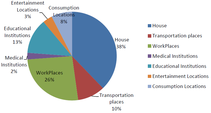
- Besides individual persons, physical locations were generated where individuals can perform a variety of activities. Currently, there are 18 location types, and these location types are classified into 6 categories: houses, educational institutions, workplaces, consumption locations, entertainment locations, and medical institutions. Each location has a geographic reference and the distribution of these locations was generated according to both statistical data and the geographic distribution of the population.
- The consistency between the individual person and the physical location was guaranteed. For example, a student of age 22 will be assigned a location which belongs to location type ’university’ rather than ’primary school’.
The statistics of the synthetic population and physical locations are listed in Table 1.
The statistical results of the generated synthetic population are shown in Figure 1 in the form of an age distri-bution. According to the previous results, the standard deviation of errors between the generated age and the statistical data is 0.9823 (95% confidence interval (CI) from 0.7034 to 1.3510).
With the generated data, Ge et al. (2014) constructed a large-scale agent-based epidemic model. Based on the same source of data, this research built a large-scale agent-based model in a new way. A key issue and challenge of utilizing the raw data to our model is the redundancy of the data, such as the agents’ preferred location list for shopping, eating and entertainment. Together with the predefined social networks for agents in the data, the size of the data is initially around 130 Gb. Since the way to implement the large-scale agent-based model in this research does not require the predefined location choices and social networks which is entirely different from Ge et al. (2014)’s method, we post-processed the raw data by extracting only the relevant fields of data items from the original database. In addition, to speed up the initialization phase, we converted the data from the database (mysql) to a compressed format (e.g., gzip) to reduce disk transfer time. With these post-processing steps, the time efficiency for loading the model could be improved by 65% in our case.

Location
With the data generated by the statistical information, we modeled each of the 8 million physical locations in the artificial city Beijing, which represent schools, restaurants, shops, hospitals, etc. The exact numbers of locations in each location type are shown in Table 2.
| Location Category | Location Type | Size |
|---|---|---|
| Houses | household | 4.961 million |
| Consumption locations | restaurant | 55257 |
| Consumption locations | market | 18686 |
| Consumption locations | mall | 547 |
| Medical institutions | clinic | 836 |
| Medical institutions | community meds | 1744 |
| Medical institutions | hospital | 569 |
| Medical institutions | medservice | 3335 |
| Educational institutions | elementary | 1090 |
| Educational institutions | kindergarten | 1305 |
| Educational institutions | middleschool | 632 |
| Educational institutions | middle university | 91 |
| Educational institutions | private university | 79 |
| Educational institutions | university | 73 |
| Entertainment locations | green | 13983 |
| Entertainment locations | playground | 6151 |
| Entertainment locations | garden | 93 |
| Workplaces | other workplace | 11431 |
Each location is characterized by its geographic reference (longitude and latitude), and the total area in square meters. The added total area parameter to a location is unique in this research, which is used to generate sub-locations (e.g., classrooms in a school) and serve as an important parameter for disease spread in the location. From Table 2, we can find that currently there are 18 location types which are categorized into 6 location categories. Apparently, these can not cover all the location types in reality in Beijing, for example, small shops in ’Consumption locations’ and cinemas in ’Entertainment locations’ are missing in the current data. Further research should be conducted on generating or collecting real data for these missing locations which are important for disease spread, as well.
We partition each location into sub-locations by giving each location an attribute ’sub-location size’. Sub-locations can represent separated classrooms in a school, stores in a shopping mall, or offices in a working place. Agents can only have direct contacts when they are in the same location and assigned the same sub-location index.
An efficient method ’calculateDistance’ is realized in the location class, which calculates the distance between two locations based on the geographic coordinate information (latitude and longitude). Since the process of calculating the distance between two locations is an indispensable step for including a transport component in the model, this method is one of the most frequently called methods during a simulation run. Thus, we optimized this method by using an approximation of one degree in longitude and latitude when transforming geographic coordinates into Cartesian coordinates. Compared with the accurate calculation, it speeds up the calculation up to 70%, while the relative errors are less than 0.5%.
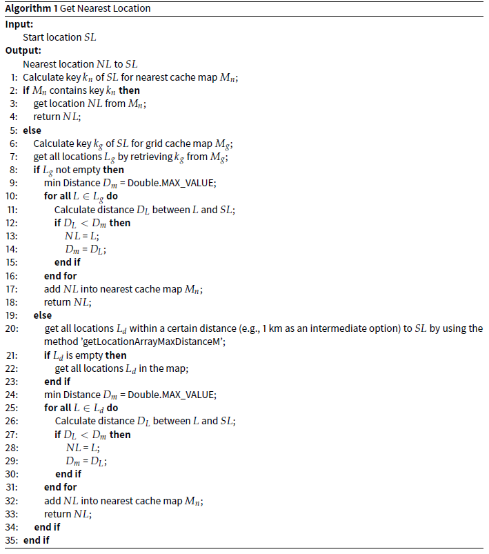
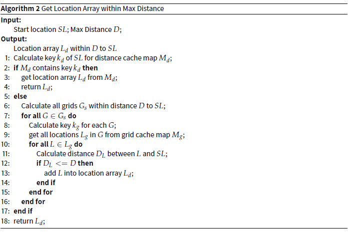
To manage the locations in each location type category, a ’LocationType’ class is created, which can be instantiated for each location type. Besides the necessary methods to manage locations, such as getting a location by index, the two most frequently called methods are ’getNearestLocation’ and ’getLocationArrayMaxDistanceM’. The first method returns the nearest location of the current location type to any location, and the second one returns an array of locations of the current location type within a max distance to any location. These two methods will be frequently called due to the fact that some people are more willing to visit the nearest places for shopping, eating and leisure when they have no particular preference. Due to the fact that most activities of agents in the simulation need to ask for a list of closest locations for carrying out that activity, calling these two methods would take a lot of computing resources.
Thus, a three-level cache mechanism was creatively designed to achieve a balance between CPU utilization and memory usage. The first cache is the nearest cache, which stores the closet location of the current location type to a certain location. New items will be added to this cache only after they have been calculated for the first time. The second cache is the grid cache. We divide the whole city map into grids and keep indexes of locations in the grids. The third cache is the distance cache, which is used when no results can be found in the nearest cache or the grid cache. To any specific location, this cache can keep nearby locations ordered by distance. Based on this design, the algorithm to implement method ’getNearestLocation’ is listed in algorithm 1, and the method ’getLocationArrayMaxDistanceM’ is listed in algorithm 2. In order to save memory for the 8 million locations, we keep the indexes of locations as values in these three caches and encode the key into a ’Long’ data type as the reference of a location.
Transportation
There are many papers on activity-based transportation simulation (see e.g. Raney & Nagel 2003; Nagel & Rickert 2001; Zhang et al. 2013). These papers mainly focus on the prediction of traffic peaks and congestions. In our implementation of the artificial city Beijing, a microscopic public transportation system is simulated and integrated with the daily activities of the population with the aim to model the ’realistic’ travel contacts.
The public transportation system is associated with the execution of travel activities, which are considered as a connection between two activities of agents in two different physical locations. An agent that has to commute by public transport between two locations to conduct its next activity, will execute a travel activity in the modeled transportation system. The transportation system will determine a route for the commuting agent and calculate the travel duration for the simulation.
The public transportation component is microscopic as we modeled all lines and stops of the metro and the bus system in Beijing. No tram lines exist in Beijing’s public transport system. We also exclude the rail train lines in this model as the trains lines in Beijing are only used as inter-city connections. During each simulation day, modeled buses and metro trains will execute their schedules on these routes based on timetables. The geographic information and routing data of the transportation infrastructure network were acquired from OpenStreetMap1 by using the Java library called Osmosis2. It offers stop information as nodes and route information as links that together form a graph. This graph shows the topology of the whole public transportation network in Beijing.
For commuting vehicles (private cars) on the road networks, the real road network was not modeled but estimated travel duration can be calculated according to the distance and historical statistical data on congestion.
The 190 metro stops and 1380 bus stops of the public transportation system are modeled as extensions of the general locations in Section 2.3. In addition to the functions of a general location, a bus/metro stop can ’move’ the waiting agent from the current stop to the arriving transporter (bus/metro train) if this transporter has enough space and is on the right route for the waiting agent in the stop. Moreover, in order to keep the agents ’simple’ enough for large-scale simulation but ’heterogeneous’ enough for public transportation, only the stops know and record transfer information of the waiting agents, and will pass the information to the transporter when the agents are on board. Then the transporter will ’move’ the agent from the bus to a stop when it arrives at the right transfer or destination stop.
Agents that transfer in/between stops cause realistic delays, while the transporter also takes a certain delay when arriving at a stop to ’move’ agents out and accept new passengers. In order to be realistic, we also enabled the bus or metro train to operate through a timetable. This data driven method enables this public transportation component to simulate people’s real travel behavior.
To enable the modeled traffic infrastructure components to offer routing information for commuting agents, a graph for routing was constructed using an open source Java library called jgrapht3 to connect the 1570 bus and metro stops. Every two stops of the same bus/metro line are linked and the edge of each link is assigned a travel duration. We also link stops that are not on the same route but within walkable distance, and assign an estimated duration by foot on this edge of the link. By default, this graph can offer a shortest (in travel duration) path to a potential public transport user. Since this graph will be called millions of times per simulated day in our model of Beijing, we added a cache in each node (stop) to store the next transfer stop information with its destination node as the key in the cache.
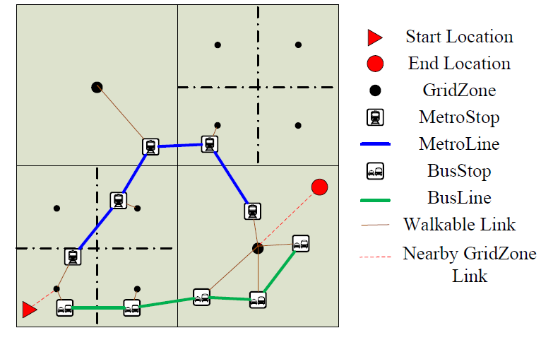
However, there is a big challenge for an agent to use this graph to get a travel route, which is to find the first stop to use as there could be more than one public transport stop close to the agent. An explicit solution is comparing all the nearby stops for every travel request. This could decrease the simulation performance drastically. We solved this challenge by creating ‘GridZones’ as nodes and adding them to the existing graph. We divided the map into grid cells, and the resolution of the grid can be set flexibly. We call the center of each cell ‘GridZones’. Each ‘GridZones’ is a node and is linked to the graph by linking the ‘GridZones’ with all stops in this grid cell. The weight of each edge is assigned an estimated walking duration. When an agent plans to use public transport, the public transportation model will use the agent’s current ‘GridZones’ as the start node to calculate the shortest path. The destination location is treated in a similar manner. The details are shown in Figure 2.
Besides public transportation, an agent can also choose to commute by his or her own private car (taxis are not included in this research). An approximate duration of commuting by cars will be given by the transportation system for the execution of the simulation.
When the location of an agent’s next activity is within walkable distance, a travel activity ’walk’ is conducted. Similar to taking a car, no actual road networks are modeled for walking agents in our model but a ’walk’ location is created instead. This enables people to meet others by chance when walking, although the probability is rather small. In our model, there is a ’walk’ location with a large area into which all walking agents will be put temporarily.
Agent
Artificial city Beijing simulates 19.6 million agents and their daily behavior. Typical implementations of agents’ behavior in artificial city research are activity-based, where all activities for the whole simulation are predefined in the input data source (Ge et al. 2014) or generated before the simulation run (Stroud & Valle 2007) which consumes a lot of memory. Assume there are around 20 million agents and each agent has 10 activities per day, then the total number of activities for a 4 weeks simulation period is 5.6 billion. To reduce memory consump-tion, we designed an agent as activity pattern based. This design is based on Mossong et al. (2008)’s research that human behavior patterns are remarkably similar among people in different countries and the patterns are highly correlated with age.
Since the age of a person is highly related to the social role (Kite 1996), each agent was given a social role (infant, student, worker, elder, unemployed) in the dataset prepared in Section 2.2. We distinguish between roles by giving agents different week patterns. For instance, a university student will be assigned one of the university student week patterns, and a worker will be assigned a worker pattern. To increase the heterogeneity and richness of these schedules, more than one week pattern are designed for each social role. A week pattern is made up of seven day patterns. For a typical worker week pattern, the first five days patterns can remain the same as weekday patterns, and the last two days can be the same as weekend patterns. In the week pattern for retired agents, the seven day patterns can be the same, for instance.
In this research, we designed around 20 different day patterns for all social roles in the artificial city Beijing, which is based on other independent research conclusions. Ta et al. (2015) distinguished the working people in the suburb area of Beijing into 5 types by recording the real GPS data and combining the difference in activity (work, eat and shop) distance and commuting frequency. To summarize, they differentiated between 5 types of workers: (1) people who work at home and seldom go out; (2) people who work and do other activities nearby (within 3 km); (3) people who do activities in average distance of 7 km to home; (4) people who do activities in an average distance of 10 km to home; (5) people who do activities further than 15 km. Based on this research, firstly we merged type (3)(4) and (5), and then separate the resulting type into 2 new types by the way of commuting to work, which are commuting by public transportation and by private vehicles. The people of the type of commuting by private vehicles were separated into another 2 new types, which are those who need to car-pool their children to school every school day and those who don’t. For workers during weekend days, 4 types of day patterns were designed according to the conclusions made by the research in Yue et al. (2013), which are: (1) people who stay at home during weekend; (2) people who do activities nearby (within 3 km); (3) people who do activities further than 3 km by public transportation; (4) people who do activities further than 3 km by driving.
For people who are retired, Ta et al. (2015) concluded that they behave mostly like Type (1) and (2) of workers. Thus, we designed 2 day patterns for them. The first type prefers to stay at home and the other prefers to do ac-tivities outside but nearby. Besides, there is no di erence for retired people between weekdays and weekends in this research. For students, due to the scarce data, 3 types of weekday patterns were designed for typical stu-dents according to the way they commute to school. For weekend days, 4 types of day patterns were designed which are similar to workers. Since the commuting ways for students are highly correlated to the distance to schools in the initial dataset and the patterns of their parents (those who carpool their children to school or to other shopping and entertainment places), the proportion of assigning patterns to students were determined by the simulation model, both for weekdays and weekends. For babies, we assumed there is only one typical day pattern for them which is associated with their parents who work at home. Since this model is used to predict epidemics, a special day pattern for hospitalized people was designed as well.
A list of all designed day patterns are presented in Table 3. An algorithm was implemented to pick the proper weekday patterns and weekend patterns to form a week pattern, and to assign the resulting week pattern to agents during the initialization phase of the simulation.
To give a detailed impression of the designed typical day patterns, a weekday pattern example for workers who carpool their children to school in weekdays is presented in Table 4, and a day pattern example for workers who drive outside during weekends is presented in Table 5.
| No | Activity Name | Activity Type | Duration |
|---|---|---|---|
| 1 | sleep | StochasticDurationActivity | Triangular (6.0, 7.0, 7.5) |
| 2 | carpool Child | CarpoolActivity | based on simulation |
| 3 | work | UntilFixedTimeActivity | until 12:00 am |
| 4 | lunch and rest | StochasticDurationActivity | Triangular (0.4, 0.6, 1.0) |
| 5 | work | StochasticDurationActivity | Uniform(4.0,7.0) |
| 6 | drive home | TravelActivityCar | based on simulation |
| 7 | walk to shop | TravelActivityWalk | based on simulation |
| 8 | shop | StochasticDurationActivity | Triangular(0.1, 0.3, 0.5) |
| 9 | walk home | TravelActivityWalk | based on simulation |
| 10 | family dinner | FamilySynchronizedActivity | Fixed(20:00-21:00) |
| 11 | housework | StochasticDurationActivity | Uniform(1.0,2.0) |
| 12 | sleep till midnight | UntilFixedTimeActivity | until 24:00 |
| No | Activity Name | Activity Type | Duration |
|---|---|---|---|
| 1 | sleep | StochasticDurationActivity | Triangular(7.5, 8.5, 10.0) |
| 2 | housework | StochasticDurationActivity | Uniform(1.0,4.0) |
| 3 | drive | TravelActivityCar | based on simulation |
| 4 | shop/entertainment | StochasticDurationActivity | Uniform(2.0,10.0) |
| 5 | eat | StochasticDurationActivity | Triangular(0.4, 0.6, 1.0) |
| 6 | drive home | TravelActivityCar | based on simulation |
| 7 | housework | StochasticDurationActivity | Uniform(0.5,2.0) |
| 8 | sleep till midnight | UntilFixedTimeActivity | until 24:00 |
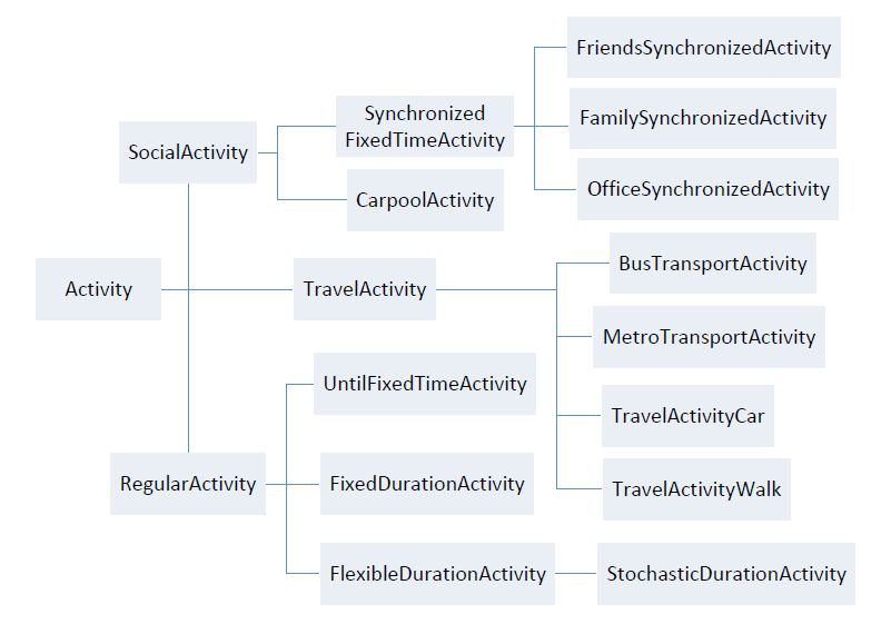
Every activity in any day pattern belongs to an activity type, and we categorized the activity types into three root categories in Figure 3, which are the regular activity, the travel activity and the social activity. Typical activities, such as sleeping, staying at home, working, shopping and attending school belong to the regular activity category.
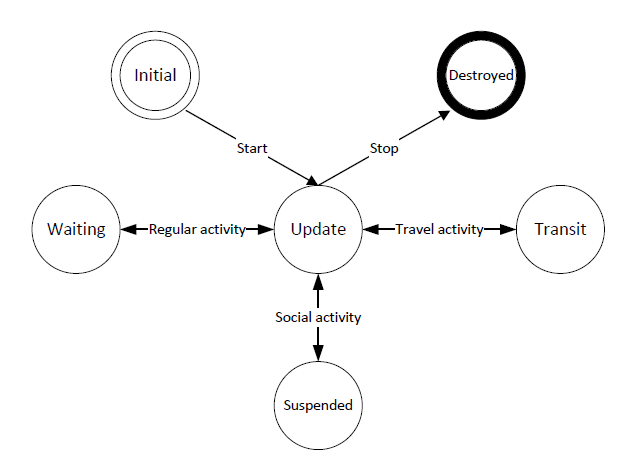
Much like the agent life cycle in a FIPA agent (Poslad 2007), an agent realized in this model has an implicit life cycle describing the agent states with the execution of activities (see Figure 4) .
The difference between the life cycle of FIPA agents and agents in this model is how states are transited. Each FIPA agent keeps the exact current state in its life cycle and needs a specific transition instruction for updating to the next state. To achieve this, every agent should maintain a list of future instructions which consumes a lot of memory. In our model, the current state of the agents is not clear as there are no explicitly defined states in the agents. Instead we keep a current activity index within the current day pattern of an agent. When executing an activity, the activity itself or activity executor (if this activity is a travel activity or social activity) will specify a duration for this agent to schedule its next activity. During this period, the agent remains in an implicit state (e.g., suspended), which is shown in Figure 4. Based on this design, the day patterns and the week patterns are reusable for agents who have the same social role, which considerably reduces memory usage compared to the FIPA solution. Take the same assumption mentioned above, assume there are around 20 million agents and each agent has 10 activities per day, then we can design 100 day patterns instead of the initial 5.6 billion activities for a 4 week simulation period, which are only around 1000 activities in total. Moreover, the week pattern of an agent in our model can be changed as a result of the state of the system (e.g., a policy intervention) as the week pattern is treated as an index attribute for an agent, which increases the flexibility of the model.
Social networks
There are three types of social networks modeled in this research, which are family, colleagues/ classmates and friendships. Family, colleagues and classmates relations can easily arise from defining a complete topology that clearly specifies all relation connections, which is shown in Figure 5.

Friendships, as the most complex social relation, are relatively difficult to define. The topology of friend connections changes over time due to the dynamics of friendship relations (Pujol & Flache 2005). This is even more complicated on a large scale (Gatti et al. 2014). Thus, egocentric friend networks are dynamically generated to represent friendship connections. In this research, friendships will be generated before planning and negotiat-ing social activities based on an algorithm that we will present below. The candidates for the friends come from three kinds of sources: neighbors, classmates/colleagues and a random selection. When agent A is planning a social activity, the algorithm for generating friends can be described as follow:
| Social role | Name of Day pattern | Proportion for the social role | Description for the typical day pattern |
|---|---|---|---|
| Infant | B_Pattern | 100% | For all babies |
| Student | S_DayWalk | Based on initial data and model | For students who walk to school in weekdays |
| Student | S_DayPT | Based on initial data and model | For students who take public transportation in weekdays |
| Student | S_DayCarpool | Based on parent’s pattern | For students who are sent by parents using cars in weekdays |
| Student | S_WeekendHome | Based on initial data and model | For students who stay at home during weekends |
| Student | S_WeekendNearby | Based on initial data and model | For students who do activities nearby (within 3 km) during weekends |
| Student | S_WeekendPT | Based on initial data and model | For students who do activities outside using public transportation during weekends |
| Student | S_WeekendDrive | Based on parents’ pattern | For students who do activities outside with parents by driving during weekends |
| Worker | W_DayHome | 12.9% | For workers who work at home |
| Worker | W_DayNearby | 12.2% | For workers who work nearby (within 3 km) |
| Worker | W_DayPT | 33.7% | For workers who take public transportation to work |
| Worker | W_DayDrive | 19.2% | For workers who drive to work |
| Worker | W_DayCarpool | 22% | For workers who drive but carpool child to school first |
| Worker | W_WeekendDayHome | 20% | For workers who stay at home during weekends |
| Worker | R_DayHome | 50% | For retired people who prefer staying at home |
| Retired | R_Dayout | 50% | For retired people who prefer do activities outside |
| Retired | R_Dayout | 50% | For retired people who prefer do activities outside |
| ALL | HospitalizedDay | based on simulation | For hospitalized people |
First, the number of friends Ns is assigned to A which follows a power-law distribution (Hamill & Gilbert 2010). According to the fact that Dunbar’s number (Hill & Dunbar 2003) ranges from 100 to 250, the largest size of friends in this research is set to the lower boundary 100 to reduce the computational complexity. The skewness is set to 0.8, which is an example experiment setting in Hamill & Gilbert (2010).
Second, the percentage of A’s friends from di erent sources is calculated according to a combination of uniform distributions (see Table 6) as the source composition of A’s friends may di er from another agent. For example, agent A may like to make friends with neighbors while agent B may prefer making new friends randomly in places like shops or restaurants.
| Item | Number |
|---|---|
| Total number | Ns |
| Number of friends from classmates/colleaguesNc | Uniform [0,Ns] |
| Number of friends from neighbors Nn | Uniform [0,Ns, Nn] |
| Number of friends from random selection Nr | Ns - Nn - Nc |
Third, select one candidate randomly from the source and calculate the possibility that the candidate and agent A are friends. If the calculation result exceeds a predefined threshold (e.g., 0.25 as an initial setting), put the candidate in agent A’s friends list. Otherwise, select a new candidate and repeat the calculation process till all A’s friends are generated. If the new friends list is still not full, increase the threshold and repeat the calculation process again. The calculation process is based on a concept called ’social similarity’, which is proposed in this paper. It calculates the similarity between two agents. The considered variables include age, social role (week pattern), family role and the number of friends. In this research, the ’social similarity’ S(A, B) between two agents A and B is evaluated by a weighted Euclidean distance which is shown is in Equation 1, where a represents age, s represents social role (converted to an index), f represents family role, n represents the agent’s friends size and m represents the weights for different variables.
| $$S(A,B)= 1-\sqrt{\sum\limits_{i=a,s,f,n}\mu_i(A_i-B_i)^2}$$ | (1) |
Architecture of the artificial city
Models of locations, agents, social networks and the public transportation component constitute the main part of the artificial city. The system architecture of the artificial city can be summarized by a class diagram containing the major classes in our implementation which is shown in Figure 6.
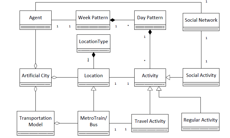
Based on this architecture of the artificial city and our research interest in this paper, we built simulations to study how spatial contacts can be modeled and observed, which will be detailed in Section 3.
Spatial Contacts
In Sect 2, we constructed an artificial city with a large population by combining diverse data sets, including generated data from census information, open map data, etc. With this model, spatial contacts emerge during the execution of the model. We will separate the spatial contacts into three di erent types and describe how each type of contact can be observed and measured in the following subsections.
The simulation of the proposed artificial city is implemented using the DSOL package (Jacobs et al. 2002) which is a Java-based discrete event simulation architecture. We ran the simulation on a PC (Intel Core i7-2620M CPU, 16.0 GB RAM) for a simulation period of 30 days.
Regular contacts
Regular contacts emerge when agents execute their daily regular activities in physical locations. For example, regular contacts can emerge among students who are in the same school location. When a student is executing a school activity, and another student is executing a school activity at the same location and the periods have overlap with each other, these two students are considered to have a regular contact in this model. More strictly, we divided a location into sub-locations. For example, classrooms are considered as the sub-locations in the school location. Hence, a student can only have regular contacts with other students when they are in the same classroom.
In addition to the household for each agent, the school (in the form of ID) is initially predefined for every student, as well as the workplace for each worker. The other locations for activities like shopping and sports are dynamically chosen according to the nearest location algorithms described in Section 2.3.
Through the execution of the simulation model, the number of people in several typical location types in a simulated weekday is shown in Figure 7, where the time of the day (0:00-24:00) goes on the x-axis. The ’others’ item in the figure represents all the other location types according to Table 2.
From Figure 7, it can be found in this model that the largest part of the population during the day time in a simulated weekday are in their workplaces.

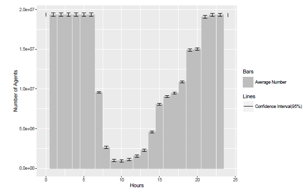
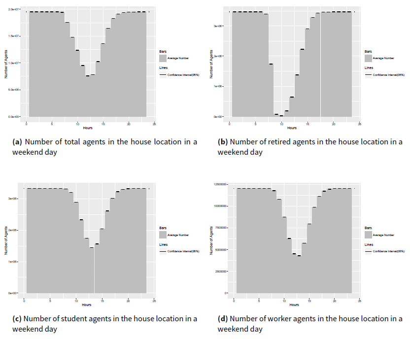
As an example, the statistical results of the hourly number of people in the house location for ten replications are presented in Figure 8, where the 95% confidence interval is drawn in the sample point (each hour).
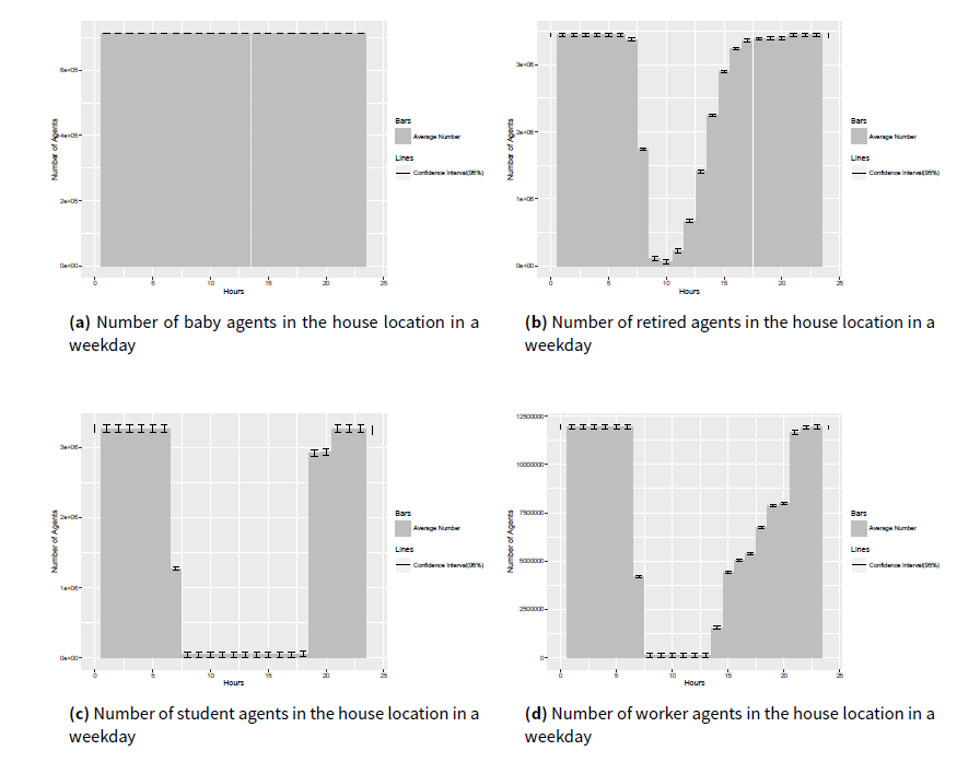
Since all the population in this research are modeled into four social roles (baby, worker, student and retired), the hourly results of agents with different role in the house location as an example are presented in Figure 9 for the weekday experiment and in Figure 10 for the weekend experiment.
In Figure 9a, we can find that the baby agents stay at home for all 24 hours. This is the result of the design of the baby pattern, in which babies are modeled to execute all activities at home. Since the results for the baby agents are the same between the weekday and weekend experiments, results are excluded for babies in Figure 10.
Due to the design of the activity in the pattern, the duration of staying in different types of locations varies among agents even when they use the same activity pattern. To verify this design, the average duration of agents staying in different locations in the weekday experiment is presented in Table 7.
From Table 7, we can find that the longest duration of stay occurs in households, followed by work or study places.
| Type | Average Duration | Standard Deviation | Confidence Interval (95%) |
|---|---|---|---|
| Household | 10.2 hours | 4.9 hours | [7.16, 13.24] |
| Mall | 0.5 hours | 0.2 hours | [0.38, 0.62] |
| Market | 0.3 hours | 0.1 hours | [0.24, 0.36] |
| Restaurant | 1.3 hours | 0.8 hours | [0.80, 1.80] |
| Workplace | 4.2 hours | 2.3 hours | [2.77, 5.63] |
| University | 6.0 hours | 3.6 hours | [3.77, 8.23] |
| Middle school | 4.5 hours | 2.1 hours | [3.20, 5.80] |
| Hospital | 0.9 hours | 0.4 hours | [0.65, 1.15] |
| Clinic | 0.5 hours | 0.2 hours | [0.38, 0.62] |
It’s not difficult to find the causal relationship between the designed 20 day patterns in Table 3for all the agents and the experiment results as a verification evaluation. To validate this design to some extent, the result of a survey by Wang et al. (2011) is used to compare with the experimental results. Wang et al. (2011) present the time-use patterns of the different neighborhood on a normal workday for workers. Based on this, two representative neighborhood, TRA and CHC are chosen. Since only workers’ result is in the research by Wang et al. (2011) and the duration in different places is simply categorized into home, out-of-home and travel, we recorded the duration for workers in different locations separately and made a comparison in Table 8, where the duration in travel is excluded.
From Table 3, we can find that the relative error of the average duration of staying In-Home between TRA (equivalent to household in this research) and the experiment is relatively high (21.3%), compared to the average duration of staying Out-of-home between TRA (13.8%) and the experiment. This difference can be caused by many factors, such as the season of the survey, the monotonicity of the surveyed neighborhood and the incompleteness of our designed activity pattern. As our interest in this research is in a new agent-based modeling method, we accept this error while more surveys on human behavior patterns in Beijing is required in future research.
| Item | Simulation results | TRA | CHC | |
|---|---|---|---|---|
| In-home | Mean | 11.4 hours | 14.5 hours | 15.6 hours |
| CI(95%) | [7.93, 14.87] | [12.14, 16.86] | [13.06, 18.14] | |
| Out-of-home | Mean | 9.1 hours | 8.0 hours | 6.9 hours |
| CI(95%) | [7.05, 11.15] | [5.83, 10.17] | [4.54, 9.26] |
| Item | Simulation results | Historical statistics |
|---|---|---|
| by bus | 7.28 million | 8.11 million |
| by metro | 4.55 million | 3.95 million |
Due to the inclusion of public transportation, agents can have travel contacts which is considered as one novel contribution in this research. Thus, the patterns of agents’ contacts during commuting are discussed in the following section.
Travel contacts
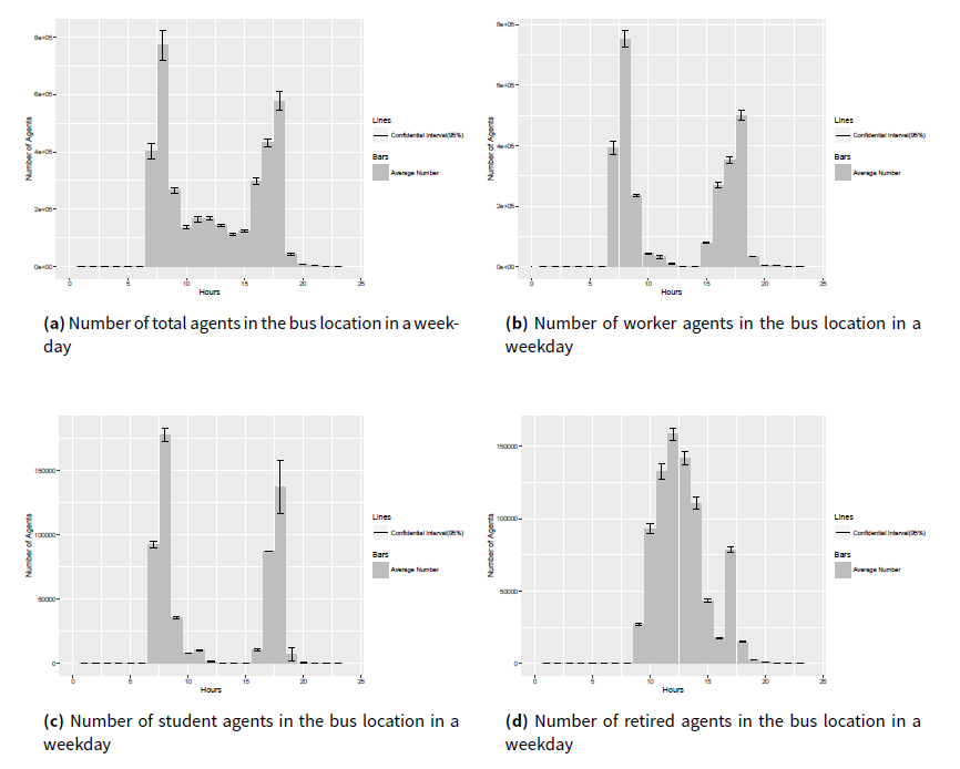
Travel contacts emerge from the inclusion of the public transportation component in this model. We observed the information on the number of people in the public transportation infrastructure components, such as metro stops, metro trains, buses and bus stops during a working day. As an example, how the numbers of agents with different social roles in the bus location change in a weekday is shown in Figure 11. Through this transportation component, travel contacts emerge. In this research, stops or metro trains are divided into several sub-locations to represent platforms or train compartments, where agents can have travel contacts when they are in the same sub-locations at the same time.
As we described before, the duration of a travel activity by bus/metro is decided by the simulation model, and is dependent on several factors, such as the travel distance, the path that the agent chooses (e.g. Dijkstra shortest path) and the waiting queue in the metro stops.
Validation of a model with a wide range of parameters would be very difficult (Stocker et al. 2001). Thus, this simulation study shi s the focus to validation using several travel statistics. In order to validate the results in this public transportation component of the whole model, the average travel volume in a weekday by bus and by metro are compared to the historical tra ic statistics report in 2011 (Guo & Li 2012) in Table 9. The reason for adopting the traffic statistics report in 2011 is to keep this research consistent as the generated population data is based on the census data of 2011.
From the comparison in Table 9, we can find that the relative errors between simulation results and the historical traffic statistics are within 15%. Several factors are responsible for the differences and one of the crucial differences is that the data collected in the report (Guo & Li 2012) only covers part of Beijing city (within the 6th Ring Road). This difference will increase the total relative errors to 28% as the daily travel volume within the 6th Ring Road only accounts for 87% of the whole travel volume in Beijing.
Regarding the travel purpose, Table 10 shows the comparison of the main purposes of using public transporta-tion in a weekday. The relative errors are less than 10%.
From Figure 11, it can be found that the rush hours for public traveling are from 7 am to 8 am and from 5 pm to 6 pm, which match the historical tra ic statistics (Guo & Li 2012).
Besides travel volume and travel purpose, travel duration is used to make a comparison for validation as well. The data for comparison comes from the survey data used in the research by Zhao et al. (2011) which presented survey data on commuting time (travel duration in this research) in a weekday conducted in a neighborhood in Beijing in 2001.
| Item | Simulation results | Historical statistics |
|---|---|---|
| For working and school | 59.2% | 54.5% |
| For shopping | 59.2% | 7.6% |
| For leisure | 6.1% | 6.5% |
| Item | Simulation results (min) | Survey data (min) |
|---|---|---|
| Mean time | 66.4 | 52.4 |
The relative errors between simulation results and the real data mainly come from the lack of certain activity patterns in the model, which results in the missing of a large amount of travel volume. For example, the model does not include patterns for business people and tourists who would use the public transportation multiple times in one day. These patterns were excluded in the model due to the lack of available data.
As a conclusion, we listed the missing components in the artificial city model that can be easily improved when the associated data becomes available.
- More refined activity patterns, such as worker pattern in night shift, tourist pattern, business people pattern.
- More rules in agents’ architecture when making decisions. For example, people in reality would consider the choice of routes based on the price of tickets before traveling while agents in this research only consider the shortest path.
- More accurate distribution of the starting time, duration and ending time of activities. For example, the departure time to workplaces for workers who are employed by universities should be earlier than those who work in restaurants in general. For now, the departure time for workers with different type of jobs follows the same distribution in this research.
Social contacts
In this paper, social contacts are defined as the contacts among agents when executing joint social activities. The challenges for modeling these contacts are manifold.
The first is that no friendship social network is predefined in the initial data. All friendship social networks should be generated before the execution process of friendship social activities based on the algorithms de-scribed in Section 2.6. For example, part of the friendship relations of agents are generated among his/her neighbors and colleagues. The reasons to generate friendship social networks dynamically for the agents are twofold: first, it is too memory-consuming to store all friends lists for all 19 million agents (up to 100 friends for each agent); and secondly, the real human friendship social networks are dynamic and evolve over time. To make this friendship relation generated by the stochastic method as stable as possible (most friends of an agent still remain the same over time), a reproducible random generator was designed using the agent id as the seed. Hence, every time when agents want to invite his/her friends to conduct a social activity in the simulation, the dynamically generated friendship relations will mostly remain the same although no static friends list are predefined, or need to be stored. The slight difference comes from the sequence of selecting candidates for friendship calculation from friends sources, which is on a first come, first served basis.
Another challenge is the consequences of the first challenge that the joint social activities are not pre-scheduled for all participants and only the organizer agent of the joint social activity foresees this activity in its schedule. Because there are no predefined friendship social networks, it is impossible to assign two consistent and semantically matched week patterns to two individual agents before the simulation starts while the two agents are modeled dynamically as friends during the simulation. This is solved through dynamically generating artificial ’Group Agents’ to help execute the friendship social activities. When the originator/organizer agent tries to execute a social activity, a helping ’Group Agent’ is dynamically generated to take over the task to execute the social activity. At first it will generate a social network, and then invite the members in the network to attend this joint social activity. After a decision tree considering several rules and conditions (for example time and distance), each invitee can either decline or accept the invitation. After collecting all the response, the ’Group Agent’ will request all the participants to travel to the social location where agents can be late due to real travel delay which is caused by the transportation model. The major process of executing a social activity is presented in Figure 12 .
The detailed interaction procedure can be described as follows:
- Before an agent starts to execute the current activity in the activity pattern, it will check the next activity to see if it is a joint social activity. If yes, check if the conditions are met for organizing it. Then a proposal of the joint social activity will be sent to all involved social networks members. It is worth noting that the friendship relations in social networks will only be generated in this step and the agent will only schedule a social activity within its current pattern.
- Calculate the attendance possibility after receiving a social activity proposal for every agent Ii according to Equation 2, where N is the total number of agents involved in the planned social activity, Io is the organizer of this activity, S(Ii, Ij) calculates the link weight between the two agents based on a concept ‘social similarity’, which calculates the ‘social similarity’ between the two agents. The considered variables include age a, social role z, family role f and the number of friends n. In this research, the ‘social similarity’ is calculated as a weighted Euclidean distance, where \(\mu\) represents the weight for different variables. By setting the weight coefficient {\(\mu_a\), \(\mu_s\), \(\mu_f\), \(\mu_n\)}, the calculation result S(Ii, Ij) will be constrained between 0 and 1. 1 means they are fully connected while 0 means no relations. A(d, E) calculates the interest degree of the activity to the agent, where d is the distance between agent's current location and proposed activity location, E gives out the degree that the agent is interested in the activity and s is a corrective coefficient for calibration.
$$\begin{aligned} & P(i,o,N) = e^{\sum\limits_{j=1,j\neq o}^N S(I_i,I_j)-N}\times A(d,E)\\ & S(I_i,I_j)= 1-\sqrt{\sum\limits_{x=a,s,f,n}\mu_x(I_{i_{x}}-I_{j_{x}})^2}\\ & A(d,E) = \frac{\sigma \cdot E}{d} \\ \end{aligned}$$ (2) - For each agent, compare the attendance possibility with its own attendance threshold t. If it is negative, send a decline response to the activity organizer and continue its own schedule. Otherwise, start the second stage process for decision-making based on a decision tree (see Figure 13).
- Two kinds of decisions can be made by the agents after the decision-tree based process, which are accept and decline. The decisions will be responded to the organizer immediately, and the organizer will make a decision on continuing the activity after collecting all responses.
- Social activity organizers will only negotiate with other members for one time, which is necessary to avoid deadlocks.
- When the final decision is made, the agents who are willing to join in the coming social activity will authorize a dynamically generated Functional Entity, ’Group Agent’, to take the responsibility for state updating and moving agents back to their original schedule when the social activity is finished.
For social contacts among family members and colleagues, the execution process of their joint social activities is almost the same as the process in Figure 12. However, the difference with the friendship social contacts is that the social networks for family members and colleagues are pre-defined in the initial data.


To evaluate the emerged social contacts, we constructed a model. The parameters in this experiment are initialized using the data from Table 12. Since the four factors (age, social role, family role and the number of friends) are considered to be equally weighted to generate a friendship link, the corresponding weight coeffcients (\(\mu_a\), \(\mu_s\), \(\mu_f\), \(\mu_n\)) are calculated according to boundary conditions, which is to enable the result S(Ii, Ij) to be constrained between 0 and 1. 1 means they are fully connected while 0 means that they have no relations. The other parameters are initialized as one possible experimental setting and the sensitivity of them will not be discussed in this paper.
| Item | Value | Description |
|---|---|---|
| \(\mu_a\) | 2.268 x 10⁻⁵ | weight coefficient |
| \(\mu_s\) | 1.563 x 10⁻² | weight coefficient |
| \(\mu_f\) | 0.0625 | weight coefficient |
| \(\mu_n\) | 2.5 x 10⁻⁵ | weight coefficient |
| A(d, E) | 1 | interest degree |
| t | 0.25 | attendance threshold |
Based on this initial setting, agents’ friends can be generated when ’FriendsSynchronizedActivity’ is scheduled during a simulation run. The number of agents’ friends is assigned to agents by the algorithm in Section 2.6 which follows a power-law distribution (Hamill & Gilbert 2010). The average number of resulted friends is around 13, which is not well validated due to the missing of actual data in Beijing.
Together with the family and the classmates/colleagues network, agents’ social networks are formed. However, agents will only generate their social networks when they need execute social activities.
Agents, who receive invitations from their friends for attending social activities which are unscheduled in their activity patterns, can make interactions with the organizing agents in order to make a final decision.
| Decisions | Equation based Process | Decision Tree based Process |
|---|---|---|
| Accept | 0.78 | 0.67 |
| Decline | 0.22 | 0.33 |
| Decisions | Equation based Process | Decision Tree based Process |
|---|---|---|
| Accept | 0.88 | 0.75 |
| Decline | 0.33 | 0.25 |
| Decisions | Equation based Process | Decision Tree based Process |
|---|---|---|
| Accept | 0.67 | 0.54 |
| Decline | 0.33 | 0.46 |
Table 13 shows the average distribution of agents’ decisions on a new family social activity after executing the processes. The equation-based process and decision tree-based process are the processes after which agents receive an activity proposal.
From Table 13, it can be found that 33% of agents decide to decline the invitation after the decision tree process.
Similar to Table 13, Table 14 shows the average distribution of agents’ decisions on a new colleague/classmate social activity. The biggest di erence between the figures is that more agents are willing to participate in a colleague/classmate social activity than in a family social activity. This is because colleague/classmate social activities are o en scheduled during the time when there are no conflicts in the agents’ schedules.
Table 15 shows the average distribution of agents’ decisions on a new social activity after executing the planning processes. Compared with the other two figures, the unusual aspect of the figure is that fewer agents accept the new proposal. This demonstrates that the composition of members in a friendship network can be heterogeneous in terms of daily schedules.
Figure 14 shows how the number of agents in different social activities changes during a typical weekday.
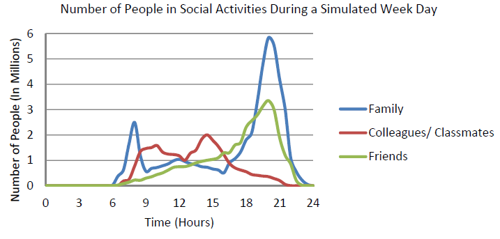
For the family social activity, there are three peaks in Figure 14 and it reaches the highest point in the evening. This indicates that people are more willing to plan activities with their families. For colleagues or students, there are two peaks in the morning and the afternoon. This is caused by the day patterns where working people have to attend meetings in the morning and afternoon and students attend joint sports activities in the afternoon. For the friend activity, it seems that most friends will only meet in the evening, to have dinner, go shopping or go to cinemas together. This phenomenon can be verified by the fact that Chinese people are more willing to have joint dinner as a social interaction (HorizonKey 2007). However, these results can’t be well validated in this paper as no independent data exists at this moment.
Modeling Disease Spread for Validation
To systematically validate the resulted spatial contact network, we implemented a pandemic influenza disease progression model on this artificial city.
Disease model
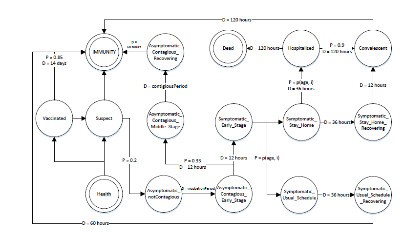
Pandemic influenza is modeled to be contagious in the resulted spatial contact networks. The phase transitions are modeled according to the research in Stroud & Valle (2007). In addition to their disease transition model, a phase called ’Vaccinated’ was added in this research, which can be used for policy modeling. The phase transi-tions and details about the transition time and probability are presented in Figure 15.
An infected agent is contagious as of the phase of ’Asymptomatic_ Contagious_Early_Stage’ until the phase of ’Convalescent’ or the end phases of ’Dead’ or ’IMMUNITY’. However, the contagious probability varies for di erent transition phases. The basic contagious rates in the phases are defined in Table 16 .
Besides the basic contagious rates, the probability to infect a susceptible person is also highly related to factors such as the space of the sub-location, the number of infected persons in the same sub-location and the contact duration. Because of this, we added more parameters in the disease progression model. The final contagious rate for a susceptible person i in a sub-location L containing N infected persons can be calculated through Equation 3, where Rj can be found in Table 16, b is a corrective coefficient for the basic contagious probability, sL is a corrective coefficient for the sub-location, SL is the space of the sub-location (in square meters) and \(t\_{ij}\) is the contact duration between person i and j.
| $$R(i,N,L) = \frac {(1 - e^{-\sum\limits_{j=1}^N \beta \times R_j\times t_{ij}}) \times \sigma_L} {S_L}$$ | (3) |
| Phase Label | Phase | P |
|---|---|---|
| RACE | Asymptomatic_Contagious_Early_Stage | 0.15 |
| RACM | Asymptomatic_Contagious_Middle_Stage | 0.5 |
| RACR | Asymptomatic_Contagious_Recovering | 0.125 |
| RSES | Symptomatic_Early_Stage | 1.0 |
| RSUS | Symptomatic_Usual_Schedule | 1.0 |
| RSURS | Symptomatic_Usual_ScheduleRecovering | 0.25 |
| RSSH | Symptomatic_Stay_Home | 1 |
| RSSHR | Symptomatic_Stay_Home_Recovering | 0.25 |
| RH | Hospitalized | 0.25 |
In this research, the corrective coefficients b and sLin Equation 1 are both set to 1.0. This simplification is determined as one possible experimental setting and the sensitivity of this set will not be discussed in this paper.
With this disease model implemented in the artificial city, a simulation was conducted to test the e ect of the modeled spatial contacts have on disease outbreak. The initial condition for the disease model was that 1 in 2 million people in the population was in the ’Suspect’ phase.
Model validation
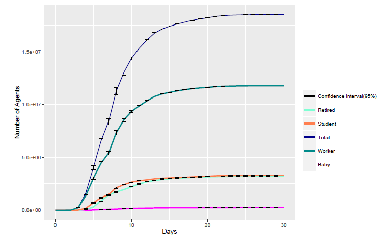
In the disease spread model, the 16 potential phases are categorized into two types: end phases and transitional phases. Firstly, we present the number of agents in the end phases of ’IMMUNITY’ in Figure 16.
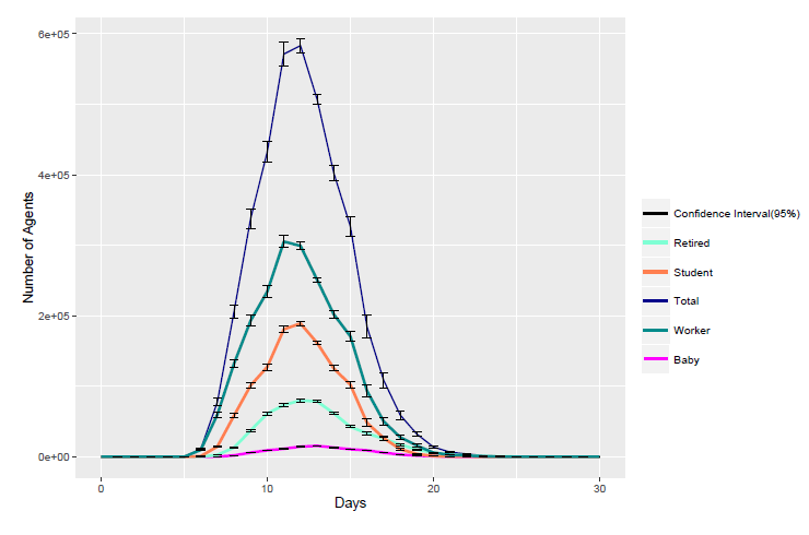
One example of the transitional phases is ’Hospitalized’, which is presented in Figure 17.
As we stated before, the phase transitions are modeled mainly according to the research in Stroud & Valle (2007). To validate the results of disease spread in this research, we made a comparison with the results of disease spread in Stroud & Valle (2007) through giving out the distribution of ’infected’ agents (from Phase ’Asymp-tomatic_notContagious’) by age group in Figure 18 and by infection location type in Figure 19.
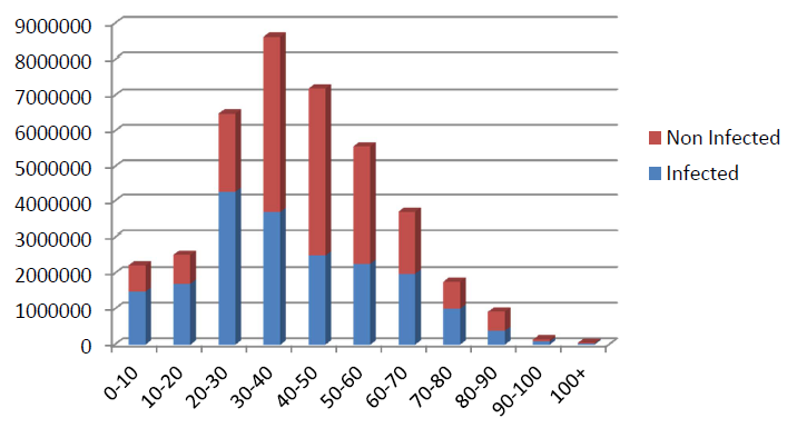
From Figure 18, we find that the age group ’10-20’ (mainly constitutes of students) got the highest infection rate which is aligned with the conclusion in Stroud & Valle (2007). CDC of the United States collected and analyzed the reported cases in 2009 and concluded that the infection rate is the highest among people in the 5 years to 24 years of age group4.
From Figure 19, we can find that household (home) is the most possible location type for disease spread among the full population, followed by workplaces, schools and transportation. This result is also consistent with the conclusion in Stroud & Valle (2007). To give a detailed view, the distribution of infected agents with different social roles in different location categories is presented in Figure 20.
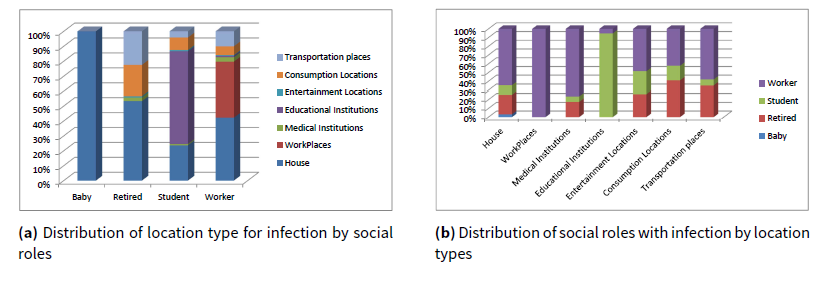
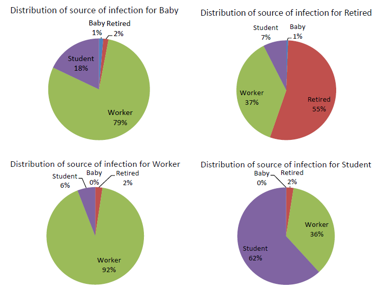
We also presented the distribution of infection sources for different social roles in Figure 21.
From Figure 21, we can find that the biggest part of the infections for a given social role are from the same social role type except for babies. It can be explained by the fact that students, workers and retired people stay with each other in most of their day time while babies always stay with their parents. Especially, workers get a higher infection possibility from their companions than the other social roles. It is caused by both the facts that workers are the biggest part of the population and workers are in more closed spaces during the day.
Although some basic disease dynamics reported in the figures above are consistent with Stroud & Valle (2007), there are many di erence in other specific indicators. For example, Stroud & Valle (2007) reported that about 10% of the population will be symptomatic or convalescing at the pandemic peak after 30 days of stable and exponential growth, while we get a result of around 5% of the population that will be convalescing after 16 days. Furthermore, there are are also difference in the concrete numerical values in terms of the the breakout of cumulative infections by location type and the clinical attack rates by age groups. Since we believe these differences are correlated to the artificial city model, and the underlying population data (China vs USA) are different, these indicators will not be validated in this research.
In reality, there was an H1N1 outbreak in Beijing in 2009 which lasted more than six months. However, the historical data, including the peak number of ’infection’ and the time of the peak, will not be used for validation in this research due to many factors. First of all, the peak number of reported ’infection’ was based on confirmed cases. These cases do not distinguish the disease phases and do not contain detailed personal information. Secondly, the reported peak time (day) lasted a rather long period as a series of interventions were conducted by di erent authorities in different part of the city among different social roles from the first case in May 16 to the peak time on October 28, 2009. Therefore, the simulated results of the extreme situation in this research cannot be validated. Instead, an expert validation process is required as part of future research.
Comparison with Related Works
Model with same disease transition model
Since this research shares the same disease (H1N1) model with the research EpiSimS by Stroud & Valle (2007) for prediction in southern California, it is meaningful to compare the model by EpiSimS with the model in this research.
Besides the differences in data and parameters such as the basic contagious rate (R0) and the data source, the major differences are reflected in the choices in the design and implementation phases.
- Although sublocations are modeled in EpiSimS, the activity locations are organized in a more hierarchical way in this research.
- Weekdays and weekend days are averaged to get a representative day in EpiSimS while they are sepa-rately modeled in this research.
- EpiSimS does not capture disease transmission during travel while this research includes a public trans-portation component for commuting.
- Agents’ behavior are based on fixed schedules in EpiSimS while both activity pattern can be replaced and specified activities (e.g., social activity) in the pattern can be rescheduled in this research.
Model with same data source
Although the population and environmental data originates from Ge et al. (2014)’s research, this research is independent and the way to design and implement the artificial city model and epidemic prediction model is different. To show how the research in this paper is unique and innovative, we made a comparison between this research and the KD-ACP framework (Chen et al. 2015) which was used to implement an epidemic model based on the same data.
- Agents implemented by KD-ACP behave according to fixed activity schedules in terms of the activity sequence, the activity locations (fixed choices) and duration. That is, agents in KD-ACP do not have decision-making capabilities. This paper models agents in a different way by which agents own multi-level decision-making capabilities while still staying "simple" and "small" enough for computational efficiency.
- Social networks in KD-ACP are predefined in the initial data, thus, no unscheduled joint social activities can be executed in the simulation. This paper generates social networks for agents dynamically by which agents can have complex social interactions in order to join in unscheduled joint social activities.
- Subway networks are modeled to represent the whole public transportation in KD-ACP. A lot of efforts are required to complete the public transportation networks. However, this paper archives this task easily by connecting traffic objects (buses and metro trains) with travel activities.
- The disease model are considered to be validated in KD-ACP in two indicators, the infection trend and the basic reproduction number. This paper verifies and validates the model in both people’s daily behavior and infection details, which include more model details.
Model with same purpose
Compared with other research (Stroud & Valle 2007; Parker & Epstein 2011; Ajelli et al. 2010; Rakowski et al. 2010; Bisset et al. 2009, 2014; Ge et al. 2013) whose research trend is on studying some of the interventions for specific interests, the contribution of this paper is mainly the proposal of a way to model relatively complete spatial contacts among a large-scale population, by which policy makers can test multiple interventions for controlling disease spread using one epidemic model. The novelty of this model consists of the following aspects:
- A microscopic public transport system (subways and buses) together with a predicted road tra ic system are simulated in an artificial city and are well integrated with the daily activities of the population.
- Social networks can be dynamically generated to execute joint social activities.
- The model is scalable (19 million agents) and can still be simulated on a PC.
Conclusions
This paper designed algorithms and approaches to model complete spatial contacts for epidemic prediction in the context of a large-scale artificial city. Firstly, by combining diverse data sets, including generated census-based data, open source maps, activity patterns, an artificial city with a large population was constructed. In this artificial city, each of the 8 million physical locations and 19.6 million citizens were modeled. All of these individuals can carry out regular activities, travel around, and join non-predefined social activities by executing their daily activities according to a pattern. With this model, spatial contact networks emerge and can be observed during the execution of the model.
Among these efforts, the activity pattern based design of agents can be considered as the foundation for modeling complete spatial contacts for epidemic predictions. With this design, the memory usage for keeping the necessary information for millions of agents can be constrained to an acceptable level while agents can still show diverse behavior in terms of activity locations, activity durations, travel routes and decisions for non-predefined social activities, even when agents have the same activity pattern. Through the execution of different types of activities in the agent patterns, the spatial contact networks emerge.
Secondly, to investigate the effect of the emerging spatial contact network for epidemic prediction, a pandemic influenza disease progression model was implemented. The results are consistent with other independent research. We believe this research and the constructed model could be an effective starting point as the model in this research can observe relatively complete spatial contacts for the first time.
Since this research can also be considered as a proof of concept which exemplifies how complete spatial contact networks in a large-scale city with complex social networks can be modeled using an agent-based method, it also indicates potential use in areas such as public transportation systems and city level evacuation planning.
As for future research, two more efforts are required to refine the model. The first is more actual data, such as adding more optional week/day patterns by surveying statistics of people’s actual activity patterns, and more surveying on distribution of people’s friends. The other is to improve the simulation performance by distributing this model, as it still takes approximately 30 hours to run one replication.
Acknowledgements
This paper is mainly based on the published PhD thesis (Zhang 2016). The authors would like to thank the National Nature and Science Foundation of China under Grant No. 91024030 and 61403402.Notes
- http://www.openstreetmap.org.
- http://wiki.openstreetmap.org/wiki/Osmosis.
- http://jgrapht.org .
- http://www.cdc.gov/h1n1flu/surveillanceqa.htm .
Appendix
References
AJELLI, M., Gonçalves, B., Balcan, D., Colizza, V., Hu, H., Ramasco, J. J., Merler, S. & Vespignani, A. (2010). Comparing large-scale computational approaches to epidemic modeling: agent-based versus structured metapopulation models. BMC infectious diseases, 10(190). [doi:10.1186/1471-2334-10-190]
BEN-ZION, Y., Cohen, Y. & Shnerb, N. M. (2010). Modeling epidemics dynamics on heterogenous networks. Journal of Theoretical Biology, 264(2), 197–204. [doi:10.1016/j.jtbi.2010.01.029]
BERNSTEIN, G. & O’Brien, K. (2013). Stochastic agent-based simulations of social networks. In Proceedings of the 46th Annual Simulation Symposium, (pp. 33–40). Society for Computer Simulation International.
BHADURI, B., Bright, E. & Rose, A. (2014). Data driven approach for high resolution population distribution and dynamics models. In Proceedings of the 2014 Winter Simulation Conference, (pp. 842–850). IEEE. [doi:10.1109/WSC.2014.7019945]
BISSET, K., Chen, J., Deodhar, S., Feng, X., Ma, Y. & Marathe, M. V. (2014). Indemics: an interactive high-performance computing framework for data-intensive epidemic modeling. ACM Transactions on Modeling and Computer Simulation, 24(1), 1–32. [doi:10.1145/2501602]
BISSET, K., Chen, J. & Feng, X. (2009). EpiFast: a fast algorithm for large scale realistic epidemic simulations on distributed memory systems. In 23rd International Conference on Supercomputing, (pp. 430–439). [doi:10.1145/1542275.1542336]
CHEN, B., Ge, Y., Zhang, L., Zhang, Y., Zhong, Z. & Liu, X. (2014). A modeling and experiment framework for the emergency management in AHC transmission. Computational and Mathematical Methods in Medicine, 2014, 1–18. [doi:10.1155/2014/897532]
CHEN, B., Zhang, L., Guo, G. & Qiu, X. (2015). Kd-acp: a software framework for social computing in emergency management. Mathematical Problems in Engineering, 2015. [doi:10.1155/2015/915429]
DEL VALLE, S., Hyman, J., Hethcote, H. & Eubank, S. (2007). Mixing patterns between age groups in social networks. Social Networks, 29(4), 539–554. [doi:10.1016/j.socnet.2007.04.005]
EPSTEIN, J. M. & Axtell, R. L. (1996). Growing Artificial Societies: Social Science from the Bottom Up. Princeton University Press.
FRIAS-MARTINEZ, E. (2011). An agent-based model of epidemic spread using human mobility and social network information. In 2011 IEEE International Conference on Privacy, Security, Risk, and Trust, (pp. 57–64). Boston, MA: IEEE. [doi:10.1109/passat/socialcom.2011.142]
GATTI, M., Cavalin, P. & Neto, S. (2014). Large-scale multi-agent-based modeling and simulation of microblogging-based online social network. In S. J. Alam & H. V. D. Parunak (Eds.), 14th International Work-shop on Multi-Agent-Based Simulation, vol. 8235, (pp. 17–33). Springer Berlin Heidelberg. [doi:10.1007/978-3-642-54783-6_2]
GE, Y., Liu, L., Qiu, X., Song, H., Wang, Y. & Huang, K. (2013). A framework of multilayer social networks for communication behavior with agent-based modeling. Simulation, 89(7), 810–828. [doi:10.1177/0037549713477682]
GE, Y., Meng, R., Cao, Z., Qiu, X. & Huang, K. (2014). Virtual city: An individual-based digital environment for human mobility and interactive behavior. Simulation, 90(8), 917–935. [doi:10.1177/0037549714531061]
GREFENSTETTE, J. J., Brown, S. T., Rosenfeld, R., Depasse, J., Stone, N. T., Cooley, P. C., Wheaton, W. D., Fyshe, A., Galloway, D. D., Sriram, A., Guclu, H., Abraham, T. & Burke, D. S. (2013). FRED (A Framework for Reconstructing Epidemic Dynamics): an open-source so ware system for modeling infectious diseases and control strategies using census-based populations. BMC Public Health, 13(1), 1–14. [doi:10.1186/1471-2458-13-940]
GRUNE-YANO, T. (2010). Agent-based models as policy decision tools: The case of smallpox vaccination. Simulation & Gaming, 42(2), 225–242. [doi:10.1177/1046878110377484]
GUO, J. & Li, X. (2012). The 2012 Beijing Traffic Development Report. Tech. rep., Beijing Traffic Research Center.
HAMILL, L. & Gilbert, N. (2010). Simulating large social networks in agent-based models: A social circle model. Emergence: Complexity and Organization, 12(4), 78–94
HAWE, G. I., Coates, G., Wilson, D. T. & Crouch, R. S. (2012). Agent-based simulation for large-scale emergency response. ACM Computing Surveys, 45(1), 1–51.
HILL, R. & Dunbar, R. (2003). Social network size in humans. Human Nature, 14(1), 53–72. [doi:10.1007/s12110-003-1016-y]
HORIZONKEY (2007). Chinese Social Pattern: A Small Circle. Tech. rep., HorizonKey.
HUANG, Y. (2010). Modeling the severe acute respiratory syndrome (SARS) outbreak in Beijing: an agent-based approach. In Proceedings of the 1st International Conference and Exhibition on Computing for Geospatial Research & Application. New York, NY, USA: ACM. [doi:10.1145/1823854.1823895]
JACOBS, P. H., Lang, N. A. & Verbraeck, A. (2002). D-SOL: A Distributed JAVA based Discrete Event Simulation Architecture. In Proceedings of the 2002 Winter Simulation Conference, (pp. 793–800). San Diego, CA, USA: IEEE. [doi:10.1109/wsc.2002.1172962]
KITE, M. E. (1996). Age, gender, and occupational label: A test of social role theory. Psychology of Women Quarterly, 20(3), 361–374. [doi:10.1111/j.1471-6402.1996.tb00305.x]
MEI, S., Sloot, P., Quax, R., Zhu, Y. & Wang, W. (2010). Complex agent networks explaining the HIV epidemic among homosexual men in Amsterdam. Mathematics and Computers in Simulation, 80(5), 1018–1030. [doi:10.1016/j.matcom.2009.12.008]
MOSSONG, J., Hens, N., Jit, M., Beutels, P., Auranen, K., Mikolajczyk, R., Massari, M., Salmaso, S., Tomba, G. S., Wallinga, J., Heijne, J., Sadkowska-Todys, M., Rosinska, M. & Edmunds, W. J. (2008). Social contacts and mixing patterns relevant to the spread of infectious diseases. PLoS medicine, 5(3), 381–391. [doi:10.1371/journal.pmed.0050074]
NAGEL, K. & Rickert, M. (2001). Parallel implementation of the TRANSIMS micro-simulation. Parallel Computing, 27, 1611–1639. [doi:10.1016/S0167-8191(01)00106-5]
PARKER, J. & Epstein, J. M. (2011). A distributed platform for global-scale agent-based models of disease trans-mission. ACM Transactions on Modeling and Computer Simulation, 22(1), 1–25. [doi:10.1145/2043635.2043637]
PELECHANO, N., Allbeck, J. M. & Badler, N. I. (2007). Controlling individual agents in high-density crowd simulation. In D. Metaxas & J. Popovic (Eds.), Proceedings of the 2007 ACM SIGGRAPH Eurographics Symposium on Computer Animation, vol. 1, (pp. 1–10). Aire-la-Ville, Switzerland, Switzerland: The Eurographics Association.
PEREZ, L. & Dragicevic, S. (2009). An agent-based approach for modeling dynamics of contagious disease spread. International Journal of Health Geographics, 8(50), 1–17. [doi:10.1186/1476-072x-8-50]
POSLAD, S. (2007). Specifying protocols for multi-agent systems interaction. ACM Transactions on Autonomous and Adaptive Systems, 2(4), 1–24. [doi:10.1145/1293731.1293735]
PUJOL, J. & Flache, A. (2005). How can social networks ever become complex? Modelling the emergence of complex networks from local social exchanges. Journal of Artificial Societies and Social Simulation, 8(4) 12: https://www.jasss.org/8/4/12.html.
RAKOWSKI, F., Gruziel, M., Krych, M. & Radomski, J. P. (2010). Large Scale Daily Contacts and Mobility Model - an Individual-Based Countrywide Simulation Study for Poland. Journal of Artificial Societies and Social Simulation, 13(1) 13: https://www.jasss.org/13/1/13.html.
RANEY, B. & Nagel, K. (2003). An agent-based simulation model of Swiss travel: first results. Networks and Spatial Economics, 3(1), 23–42. [doi:10.1023/A:1022096916806]
RONALD, N., Dignum, V., Jonker, C., Arentze, T. & Timmermans, H. (2012). On the engineering of agent-based simulations of social activities with social networks. Information and Software Technology, 54(6), 625–638. [doi:10.1016/j.infsof.2011.12.004]
SAWYER, R. K. (2003). Artificial societies: Multiagent systems and the micro-macro link in sociological theory. Sociological Methods & Research, 31(3), 325–363. [doi:10.1177/0049124102239079]
SINGER, H. M., Singer, I. & Herrmann, H. J. (2009). Agent-based model for friendship in social networks. Physical Review. E, 80(2), 1–5. [doi:10.1103/PhysRevE.80.026113]
STOCKER, R., Green, D. & Newth, D. (2001). Consensus and cohesion in simulated social networks. Journal of Artificial Societies and Social Simulation, 4(4) 5: https://www.jasss.org/4/4/5.html.
STRAIF-BOURGEOIS, S., Ratard, R. & Kretzschmar, M. (2014). Infectious disease epidemiology. In Handbook of Epidemiology, (pp. 2041–2119). Springer. [doi:10.1007/978-0-387-09834-0_34]
STROUD, P. & Valle, S. D. (2007). Spatial dynamics of pandemic influenza in a massive artificial society. Journal of Artificial Societies and Social Simulation, 10(4) 9: https://www.jasss.org/10/4/9.html.
TA, N., Chai, Y. & Guan, M. (2015). Suburbanization, daily lifestyle and space-behavior interaction in Beijing (in Chinese). Acta Geographica Sinica, 70(8), 1271–1280.
WANG, D., Chai, Y. & Li, F. (2011). Built environment diversities and activity–travel behaviour variations in Beijing, China. Journal of Transport Geography, 19(6), 1173–1186. [doi:10.1016/j.jtrangeo.2011.03.008]
YUE, S., Yanwei, C. et al. (2013). Daily activity space of suburban mega-community residents in Beijing based on GPS data (in Chinese). Acta Geographica Sinica, 68(4), 506–516.
ZHANG, L., Chang, G., Zhu, S. & Xiong, C. (2012). Integrating an agent-based travel behavior model with large-scale microscopic traffic simulation for corridor-level and subarea transportation operations and planning applications. Journal of Urban Planning and Development, 139(2), 94–103. [doi:10.1061/(ASCE)UP.1943-5444.0000139]
ZHANG, L., Yang, W., Wang, J. & Rao, Q. (2013). Large-scale agent-based transport simulation in Shanghai, China. Transportation Research Record: Journal of the Transportation Research Board, 2399, 34–43. [doi:10.3141/2399-04]
ZHANG, M. (2016). Large-Scale Agent-based Social Simulation - A study on epidemic prediction and control. Ph.D. thesis, Delft University of Technology.
ZHAO, P., Lü, B. & De Roo, G. (2011). Impact of the jobs-housing balance on urban commuting in beijing in the transformation era. Journal of Transport Geography, 19(1), 59–69. [doi:10.1016/j.jtrangeo.2009.09.008]
ZHAO, Y. & Sadek, A. W. (2012). Large-scale agent-based traffic micro-simulation: Experiences with model refine-ment, calibration, validation and application. Procedia Computer Science, 10(2), 815–820. [doi:10.1016/j.procs.2012.06.105]