
Introduction
Computational methods are slowly gaining wider acceptance as a viable research process for organizational theory and behavior (Davis, Eisenhardt, & Bingham 2007; Harrison et al. 2007), among other social science disciplines. For instance, computational models have been used to explore the complicated dynamics of self-regulation and goal selection (e.g., Vancouver, Weinhardt, & Schmidt 2010; Vancouver, Weinhardt, & Vigo 2014). Before computational modeling, researchers would think through their theories and mentally simulate their consequences, using what Einstein called “thought experiments” (Norton 1991). But with computational models, researchers are able visualize their theoretical propositions in an interactive way and thus understand the complex interacting dynamics of their theory, something that is notoriously difficult to do in one’s head (Weinhardt & Vancouver 2012). Often, simulations of computational models (e.g., systems dynamics or agent-based models) show the researcher surprising and unanticipated emergent behavior. Because of this, recent work has argued that computational modeling is an underutilized tool for exploring intra- and inter-individual processes (Vancouver & Weinhardt 2012; Weinhardt & Vancouver 2012). However, journal reviewers are often hesitant to embrace the method, making it difficult for simulation researchers to publish in top-tier journals.
In this paper, we argue that the slow acceptance of computational modeling as an aid to theory building stems from two practical problems that are deceptively simple: equifinality and reasonable assumptions. Equifinality refers to a characteristic of general systems where two systems with different initial conditions and different internal processes may arrive at indistinguishable outputs (von Bertalanffy 1968). Reasonable assumptions are the decisions made while operationalizing abstract concepts into those initial conditions and internal processes. Equifinality and reasonable assumptions are straightforward concepts that most researchers intuitively grasp. But, perhaps because they are so straightforward, there has been little work discussing how these concepts affect how computational modelling is used for building theory.
The goal of this paper is to explore the problems of equifinality and reasonable assumptions, and demonstrate their importance in concrete terms. First, we describe computational modeling and discuss computational modeling’s double edged sword: that the principle advantage of simulation for theory-building (its concreteness) is also its disadvantage. We use a simulation of a classic small group study by Alex Bavelas to demonstrate the problem. Ironically, using a meta-simulation to demonstrate the problems of computational modelling is an example of one of the benefits of using computational methods. This is an important problem because computational modeling has the potential to benefit organizational theory and behavioral research (Davis et al. 2007; Harrison et al. 2007; Weinhardt & Vancouver 2012), but non-simulation researchers often question its value. In this paper we show that questions about the value of computational modelling are legitimate and important. We conclude with two recommendations for how computational modeling might address these concerns and gain legitimacy in the eyes of the wider community.
Using Computational Modeling for Building Theory
To understand the steps of computational model building that give rise to the equifinality problem, we first present a model of the researcher’s process in Figure 1 (this is a simplified model of the processes described by Davis et al. 2007; Epstein 1999; Harrison et al 2007; Levitt 2004; Vancouver & Weinhardt 2012; Weinhardt & Vancouver 2012).
The cognitive/verbal theory (CVT) is the term used to describe the researcher’s mental model of how a phenomenon works (Vancouver & Weinhardt 2012; Weinhardt & Vancouver 2012). The term theory here can be troublesome, as it can be used to describe a complete symbolic representation of any set of propositions and relationships. Instead, as Vancouver and Weinhardt use it, a CVT is the researcher’s model of the behavior of the system under study. For example, in one part of a real-life experimental task studying how groups make decisions, participants may be asked to choose between 3 and 4. The researcher may believe that participants would pick “randomly.” Then, “picking randomly” is the researcher’s CVT of how that particular participant works. The complete CVT of the system under study would include all the participants, all the rules governing the group’s decision-making process, and so on.
Suppose then that the researcher wishes to learn about their CVT and explore its unanticipated consequences and complex interacting dynamics. The researcher must translate the CVT into the code of the computation model (CM). In the translation process, the terms and relationships of the researcher’s CVT are operationalized as the concrete structural relationships, variables, and initial conditions of the CM. The CM can be any type of mathematical or computational approach, and requires complete specificity before it works. For example, the CM could require the CVT to be translated into the deterministic calculus used in systems dynamics models, or into the probabilities and conditional statements used in agent-based simulations (for a review of the popular approaches, see Davis et al. 2007; Harrison et al. 2007).

A taxonomy of modeling purpose
A computational model can be built for a number of purposes. There is a strong case to be made that there is theory-building value simply in the process of translating a cognitive model into a computational model and working through the dynamic implications of that complex system (Davis et al. 2007; Weinhardt & Vancouver 2012). On the other hand, for purposes such as prediction and explanation of a real world phenomenon, the simulation output would need to be carefully validated and shown to be able to produce what has already occurred (postdiction; Taber & Timpone 1996). Thus, the purposes are presented as a hierarchical taxonomy in rough order of the least stringent external validation requirements (theory-building) to most stringent (explanation). There is no other implication implied by the ranking; theory-building is not considered less important or less worthy a goal than prediction. Examples of the taxonomy are given in Table 1.
| Purposes | Benefits | |
| Explanation | existence proof possible explanation | viability of CVT to generate real-world system (generative sufficiency) |
| Prediction | predict the real-world system behavior, especially dynamics | predict consequences of changes |
| Exploration | implications of theory/assumptions curvilinear/dynamic relationships emergent properties of system | experimentation/what-if analysis falsify propositions resolve disputes |
| Generation | source of new ideas guide data collection | highlight areas of contention between theories |
| Theory-building | specificity/concrete/unambiguous variables must be operationalized internally consistent sufficiently specified | generalizations/commonalities among disparate theories clarity/transparency communication |
It is important to note that explanation is placed here above prediction. This is an arguable and strongly contentious issue (especially in the philosophy of social science simulation, e.g., Grune-Yanoff & Weirich 2010; Hofmann 2013). Our reasoning is that a simple model can be a very good predictor of a far more complex target. For instance, as the social science with the strongest record of validation and prediction, economists have long understood that a model that predicts a system may be based on entirely unrealistic assumptions (Friedman 1953)[1]. Thus, a prediction model may be externally valid without pretending to be an explanation for the system it predicts. But it would be harder to make the case that an explanatory model explained how a system worked, but did not predict its behavior at least as well as a predictive model[2]. Or in other words, external validity may be considered a necessary but insufficient condition for explanation. Our paper will focus on level 1 of modeling use (theory-building), though it is likely that the problems affecting level 1 would also affect the higher levels.
The taxonomy has the benefit of clarifying where the methodological fronts lie. Computational researchers on the cutting edge of the field have argued that simulation can be used for prediction and explanation, and thus methodological work has been concerned with establishing the bona fides of simulation for the upper levels of the taxonomy (e.g., Hassan et al. 2013). With this goal in mind, a long line of research has focused on external validation and internal verification (e.g., Balci 1998; Landry, Malouin, & Oral 1983; Mihram 1972; Yilmaz 2006).
However, mainstream work has tended to argue that the lower levels are more methodologically defensible (e.g., Davis et al. 2007; Harrison et al. 2007; Vancouver & Weinhardt 2012). Key to the lower levels are the steps related to the translation process: model building, verification, and theory-building (Harrison et al 2007). Given that mainstream research sees this as the unique value of computational modeling, we would like to focus on this translation process. Our purpose is to demonstrate that the translation process itself, while often taken for granted, has a surprising and vital impact on a computational model’s usefulness for theory-building.
The translation process: A PDCA cycle
We have broken down the translation and internal validation process into a Plan-Do-Check-Act (PDCA) cycle presented in Figure 2. The PDCA cycle (Moen & Norman 2010) is a useful analogy because it highlights that computational modeling is an iterative process. The cognitive/verbal theory (CVT) and the computational model (CM) change one another in a reciprocal cycle as the researcher constructs, learns, and experiments with the CM (Harrison et al. 2007). This is similar to how good grounded theory should be constructed (O’Reilly, Paper, & Marx 2012), and similar to the plan-code-test, or plan-test-code cycle encouraged in agile software development (Reeves 2005).
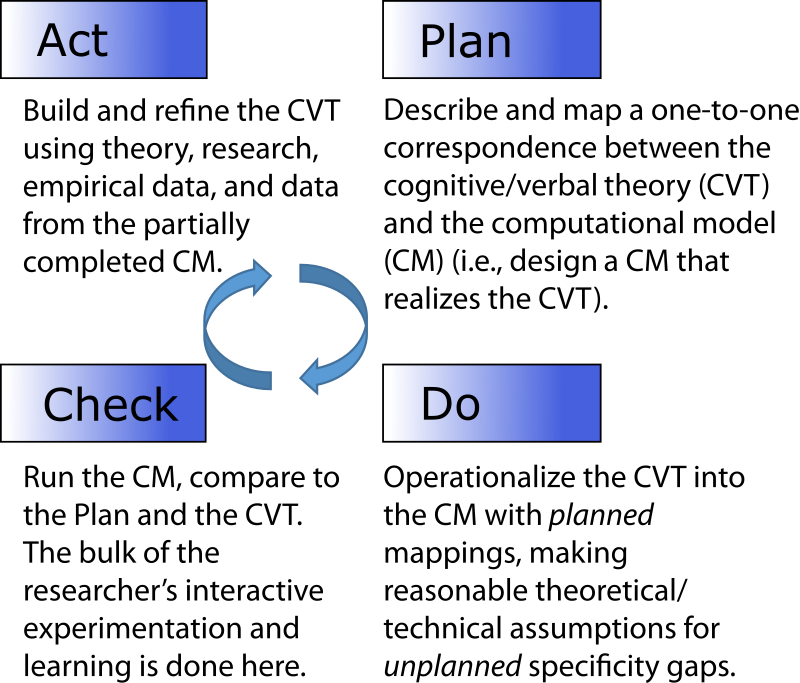
The Plan and Do stages are typically treated as the same stage (e.g., combined as “development” in Harrison et al. 2007). Here we separate them to highlight two distinct stages in the translation process. In the Plan stage the researcher establishes a correspondence between the CVT and the CM. The planning process involves mapping (operationalizing) theoretical constructs onto proposed variables, relationships, and structures. A formal design document may be produced in this stage, but often the plan exists in rough form on a whiteboard or in the researcher’s head. Although the researcher may initially believe he or she is translating the abstract CVT to the concrete level of the CM, the plan stage is in truth only an intermediate step. It is a plan in the sense that if all things go as hoped, the CVT will be accurately represented in the CM at a one-to-one correspondence.
In the Do stage the researcher converts the plan into code. This is where the rubber meets the road in the sense that the researcher is forced, by the specificity required by the modeling language, to be exact. It is possible that the plan is perfectly translatable to the context and language of the computational environment. That is, there is not a single change required in the plan, nor is there a single unanticipated decision. We believe, in practice, this would be rare indeed. The problem is that computational environments require an unanticipated level of exactness, opening up specificity gaps. Of course, this is the great benefit of simulation as a methodology (Vancouver & Weinhardt 2012). Unintended abstraction and imprecise words are not allowed here.
In the Check stage the researcher simulates the CM to see if it works. First, the researcher needs to verify that the model produces sensible output and the dynamics perform as expected. Humans are surprisingly poor at understanding and predicting complex dynamic systems (Schöner 2008; Weinhardt & Vancouver 2012). Simulations help because they allow us to explore the dynamic consequences of our theories and observe their unanticipated or emergent properties (Bonabeau 2002; Epstein 1999). For some methodological theorists, this experimentation occurs at the end of the simulation building process. But we contend that it is during the Check stage that the researcher does the core of their interactive experimentation and learning. The researcher learns about the dynamic aspects of the CVT they are trying to implement. Perhaps more importantly, the researcher learns about what works and what doesn’t when trying to close the specificity gaps of the Do stage. The Check stage is performed frequently, sometimes multiple times per minute, as the researcher iterates through the PDCA cycle.
In the Act stage the researcher makes adjustments to the CVT-to-CM plan, based on what she has learned. This may involve consulting literature, comparing to empirical data, gathering new data, or thinking. The adjustments made at this stage are typically at a higher level of abstraction than those in the Plan and Do stage, as they involve changing the researcher’s understanding of her CVT. This may be the most fruitful stage for building theory. However, note that any value-added to theory-building is dependent on the quality of the Plan and Do stages, because without a correct translation of the CVT into the CM, the information the researcher uses in the Act stage will be incorrect. This is key to the problems we highlight below.
Viewing the modeling process as a PDCA cycle reinforces the reciprocal and mutually beneficial nature of cognitive/verbal theory-building and computational modeling. In particular, the specificity required by the CM (Do stage) and the ability to test the consequences and implications of one’s CVT (Check and Act stages) are especially powerful. The benefits also lead to the double-edged sword of simulation for theory-building.
The Double-Edged Sword: Equifinality and reasonable assumptions
Equifinality is a term coined by Ludwig von Bertalanffy to describe systems, which “as far as they attain a steady state, this state can be reached from different initial conditions and in different ways" (1968). In organizational studies it means that different initial conditions and different processes can lead to the same final result (Katz & Kahn 1978 p. 30). For those trying to detect how initial conditions and processes (e.g., structural contingencies) lead to organizational performance, equifinality is a particularly vexing problem because empirical results show that a certain outcome can be the result of a number of different structures (Fiss 2007; Gresov & Drazin 1997). This is a characteristic of complexity in general (the more complex a system, the more ways inputs can result in any particular output), and complex adaptive systems in particular (internal processes that use negative feedback to maintain output stability).
The problem that equifinality poses for external validation is well known, though often ignored (Oreskes et al. 1994; Webb 2001). Simply put, if two black-boxes are able to reach identical outcomes, can we say anything at all about the similarity of their processes? In response to this philosophical quagmire, researchers endorsing computational modeling tend to focus on the lower three purposes: generation, exploration, and theory-building (Davis et al. 2007; Harrison et al 2007; Vancouver & Weinhardt 2012).
However, the PDCA cycle highlights a potential problem: the detail required by the CM far outstrips that provided by the CVT. We call this a double-edged sword because it is both the primary reason why a researcher would want to use a computational approach for theory-building, and also a strong and unresolved challenge to its use in theory-building.
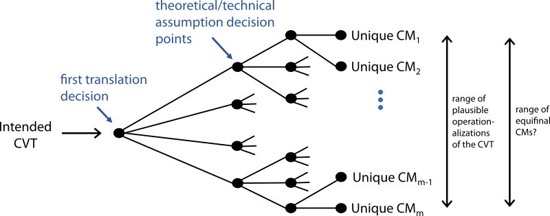
To illustrate, consider the point of view of a researcher starting with an initial computational model (the first decision point on the left of Figure 3). In the Plan stage the researcher has a proposed mapping between the CVT’s concepts and the CM’s modeling language. But it is not until the Do stage that the researcher sees the unanticipated specificity gaps. The researcher (or often the programmer!) then fills these specificity gaps with reasonable assumptions—choices made without thinking because they appear so minor and straightforward.
Assumptions can be usefully classified as theoretic or technical. Reasonable theoretic assumptions may serve as additional information for the underspecified aspects of the conceptual model. In sharp contrast, reasonable technical assumptions are made solely to satisfy “‘technological’ factors that are not really part of the hypothesis, in the sense that they are there only to make the solution possible, not because they are really considered to be potential components or processes in the target system” (Webb 2001 p. 1036).
Technological assumptions are deceptively dangerous. Instead of being based on the underlying theory of the experiment, they are a constraint of the computational language or simulation technology. For example, the researcher needs to decide which list or sorting algorithm to use, or whether int, long, or extended long types are more appropriate to hold a numerical variable. Although theoretically every Turing complete computational language could represent any possible CVT. However, practically, a computational language affords some designs and discourages others. For example, it is possible to model agents in a systems dynamics model (e.g., Vancouver et al. 2010), but there are more appropriate modelling languages if the goal was to simulate hundreds of these agents interacting in a physical space. The point is, that small decisions forced by a constrained modeling technology (such as choosing a long over an extended long) are almost never disclosed in the documentation, let alone the published literature. Yet these reasonable assumptions can have a measurable impact on the results of the simulation (as we discovered below).
Reasonable assumptions lead to equifinality, and may critically degrade the usefulness of CMs for theory-building. To illustrate, consider each assumption as a decision point in a tree. If graphed, at each decision point the tree of possible models splits based on the number of plausible choices (the left half of Figure 3). The researcher makes one assumption, follows the tree down one branch, then makes another assumption, and so on, until reaching one of the possible operationalizations of the CVT. The problem is this: many other equally reasonable and defensible assumptions could have been made at each decision point. Thus, there is a range of alternative CMs that are just as reasonable. It would be fair then to ask how many of the other equally reasonable CMs could be a plausible instantiation of the original CVT. We believe this is an unresolved problem of using computational models for building theory. In the following section we will use a meta-simulation as a concrete example of this problem.
The Meta-Simulation: A Concrete Example of the Problem
How serious should we take the problems of equifinality and reasonable assumptions? Is it a philosophical debate, or a practical problem? To answer this question, we describe our experience building a computational model of a classic social psychological experiment. We use this model to simulate the computational modeling process itself. We call this a “meta-simulation” of the computational modelling process. We built 90 other CMs, and each was an equally plausible operationalization of our original cognitive/verbal theory (CVT). That is, each CM was an end-point on the decision tree generated by the reasonable assumptions made while translating our original CVT into a CM (see Figure 3). Thus, the meta-simulation is a concrete example of simulation’s double-edged sword—it shows the benefits and the challenges of using computational modelling to explore theory.
The project: Using a computational model to build theory of an individual’s behavior in group decision-making
We began a project to build a computational model of a classic small group study by Alex Bavelas[3]. In this experiment, Bavelas took five participants, constrained their communication to zero and gave them a group goal: a target number, 17. In round one, the group members individually picked a number (their choice for that round) and submitted their choice in secret to the experimenter. The sum of the choices was the group's collective guess for the round. If the group did not reach the goal, they were told they were incorrect and given another round. For example, suppose the five members chose 3, 4, 3, 4, and 4 (for a sum of 18). They would have been given another round. Suppose then they chose 3, 4, 2, 5 and 3 (for a sum of 17). In this case the goal would have been reached in two rounds. The experiment was designed to study group decision-making ability under different information conditions (ref. personal communication with the second author).
We chose to build a CM of the “no communication” condition of this experiment. With no communication, the participants could be modeled as simple decision-making agents. A game runner would collect the agent guesses, sum the answer, and start a new round if the group failed to meet its goal. What could be simpler?
The output of the simulation for one game was the number of rounds it took to reach the target. If the simulation was run 10 times (10 runs) there would be 10 data points representing the simulation’s output distribution, which could then be compared to a target output distribution. This is how organizational behavior simulations are typically validated when used for theory-building (e.g., Vancouver et al. 2010). A group size of 5 and a target of 17 was used for the remainder of this paper.
The process of building the meta-simulation
The goal of the meta-simulation was to construct a number of plausible operationalizations of our original CVT, and validate those plausible CMs against the target “true” CM. Thus, we needed to create a “true” target CM to compare against. We chose the simplest operationalization of the CVT to be the target CM.
As we built this target CM, we took note of the reasonable theoretic and technical assumptions made during the Plan and Do stages of the modelling process (see Figure 2). As depicted in the branching diagram in Figure 3, we noted each point where we needed to make a reasonable assumption. However, instead of choosing only one assumption (as a researcher would do in a typical model building process), we made each available assumption. This branching process resulted in 90 models.
Importantly, each of the 90 models could have been a plausible operationalization of our starting CVT. This is because each choice made in the branching process could have been defended as a reasonable assumption. Each of the 90 models could have been called the “correct” CM operationalization of the original CVT. The benefit of this meta-simulation, of course, is that we already have a “one true CM.” We then asked a simple question: would it be possible, using statistical tests common in the literature, to tell which of these plausible CMs was the true CM that we had originally created?
The following sections will give a summary of some of the theoretical and technical assumptions we needed to make. It is important to note that we were forced to make these reasonable assumptions by the specificity required by the computational modelling language, and this is one of the key benefits of the computational modelling process. As we argue, however, it also one of the key dangers of computational modelling, because any realistic modelling project would have many times more assumptions than we encountered. And we have yet to see another research project document their reasonable assumptions or possible reasonable final CMs.
Reasonable theoretic assumptions
Our initial cognitive verbal theory (CVT) was our theory of how a rational participant would perceive their task and make their decision. Recall that in the no-communication condition, groups of five participants needed to collectively choose numbers that would sum up to 17. Thus, we assumed a rational actor would understand that each participant would need to pick either 3 or 4, and whether or not the group hit 17 would depend partly on luck. Our CVT stated that a rational participant would choose randomly between 3 and 4 each round until the group hit their target. We planned to model participant agents in a general-purpose programming language. A game-runner agent would poll each of the participants, gather the results, and stop the game once the group reached its goal.
However, operationalizing the concept of “random” is where we encountered our first significant mismatch between our CVT and the specificity required by the programming language. Simply put, it is difficult for a person to choose randomly. While translating our random-choosing agent into code, we crossed decision points where we needed to make reasonable theoretic assumptions about how the agent thinks about this choice. For example, considering that groups may go through many rounds before hitting the group goal, does the participant’s random choice in the current round depend on her choices in previous rounds? Suppose a participant randomly chooses 3 in Round 1. Is Round 2’s choice random between 3 and 4? Or is 4 weighted slightly more in her mind? Picking 3 twice in a row doesn’t feel as random as 3 then 4. Would three 3’s in a row be completely out of the question? How many rounds should a participant consider when deciding if a current round’s choice is random enough (i.e., what is the size and accuracy of a participant’s memory)? Are the choices made in early rounds as important as the choices made in recent rounds (i.e., primacy and recency effects)? Does random mean exactly half of the choices are 3 and half are 4? Should the length of the game affect how strict the agent is in adhering to their ideal of randomness (i.e., acquiescence)?
As one can see, there are dozens of possible ways to operationalize the concept of a “random-choice” agent. There were also a number of technical choices we needed to make while translating the CVT into a final CM.
Reasonable technical assumptions
A technical assumption includes any decision required by the specificity of the computational modelling language. Technical assumptions included: should agents be represented as objects or as data structures operated on by functions? What precision should be used for division, or what types should hold rational numbers? As can be seen, these are decisions that are not considered in the formulation of the CVT, because they are meaningless outside the domain of the computational modelling language. Yet, technical assumptions can significantly affect the behavior of the CM.
The concept of randomness included its own set of technical assumptions. Suppose we made the reasonable theoretic assumption that an agent chooses “purely randomly” between 3 and 4. When coding this Plan in the Do stage (see Figure 2) we encounter a problem: there is no “purely random” for a computer. Computers use pseudo-random number generators, so-called because they are deterministic algorithms that need to be “seeded” with an initial number. If the pseudo-random number generator is seeded with the same number, it will produce the same string of random numbers. Recent attempts to create true randomness rely on measuring atmospheric radiation instead of algorithms (Haahr 2016).
Other technical assumptions needed to be made after learning how the computational modelling language represented numbers. Recall that in the original experiment, agents have to choose whole numbers. Suppose one participant makes a random choice between 3 and 4 if their share of the total is >= 3.4 and <= 3.6. During testing, the program behaved strangely when the agents were given a share of 3.4. It turned out that the value 3.4 was stored as a floating-point type with a value of 3.3999999999. Therefore the agent always chose 3—very different behavior from the plan. Despite how common these types of floating-point arithmetic problems are, it is considered an esoteric subject even by computer scientists (Goldberg 1991).
Any other technical or theoretic assumption has the potential to create similar problems with similar drastic effects on the CM behavior. This is one example of how reasonable assumptions made in the Do stage can lead to a mismatch between the CVT the researcher thinks she has captured in her CM, and the actual CVT modelled in the CM.
The design of the meta-simulation
As discussed in the theoretical assumptions section, there were dozens of possible ways to model a participant’s decision strategy. For the meta-simulation, we chose to model only five decision strategies, in the interests of tractability (detailed in Table 2). Each of these decision strategies is a computational model of how a real participant in the Bavelas experiment might arrive at their choice. In other words, a particular decision strategy is simply one reasonable assumption we could have made while translating the original CVT into a final CM.
| Strategy | Description: If group’s goal is 17, and there are 5 participants, the agent’s share is 3.4. How will the agent decide? |
| Random (Ra) | Choose randomly between ceiling (4) and floor (3). |
| Intuitive (In) | Choose floor if fraction is < .4, choose ceiling if > .6, choose randomly otherwise. Choose floor. |
| Logical (Lo) | Choose randomly, weighted based on fraction. Choose 3 with probability 0.6, choose 4 with probability 0.4. |
| Memory (Me) | First round act as Random agent, then do opposite of last round’s choice. |
| Corrector (Co) | Using a model of other four participants, predict what they will do and then choose the amount needed to reach the goal. E.g., with a model of four Ra’s, they might choose 4, 3, 4, 4, so choose 2. |
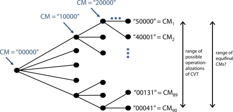
The five agent strategies allowed us to describe a final unique operationalization in terms of that CM’s combination of five agents. Using the order: Ra, In, Lo, Me, Co, a model with three Ra, one Lo, and one Co agent would be a “30101” model. Thus, a concrete example of the decision tree in Figure 3 is given in Figure 4. Each final operationalization of the CVT is a unique combination of agents, which together represent the CM if the researcher had made those particular reasonable assumptions.
Recall that our original CVT theorized that participants would choose randomly. Therefore, the meta-simulation used the five Ra agent type model (“50000”) as the hypothetical “true” model. We created 90 alternative reasonable models by producing all combinations of agent types under the following constraints: 5 agents, a maximum of 1 Co model, and if a Co model is present it is given an accurate mental model of the other 4 agents[4].
In computational modeling for theory building in fields such as organizational behavior, after a plausible CM is created, the researcher would compare the CM to the CVT or the real-world system output. For example, a qualitative validation could involve comparing event streams: if the simulation can produce a stream that is visually similar to the target stream, the CM would be a candidate explanation for that CVT. But a more stringent test would be statistical matching (e.g., Vancouver et al. 2010, 2014). Three recommended tests, and the ones used in the experiments below, are the Wilcoxon-Mann-Whitney (W-M-W), Kolmogorov-Smirnov (K-S), and the two-sample group means t-tests (e.g., Axtell et al. 1996; Balci 1998; Banks, Carson, & Nelson 1996; Law & Kelton 2000).
In summary, reasonable assumptions can lead to an exponential number of equally plausible CMs (e.g. Figure 4). At each decision point, the decision is not anticipated by the original CVT, or too technically specific to be included in the design documents. Thus, these assumptions are typically not reported in the final paper. We contend that our meta-simulation’s various candidate models are qualitatively quite different, and likely more different than the plausible CMs most modelling projects could also create. Thus, we propose that statistically comparing them to the hypothetically “true” CVT model (“50000”) would be a conservative test of the impact of reasonable assumptions on other modelling projects.
Experiment 1: Will the real CVT please stand up?
Experiment 1 asked the question: can the meta-simulation determine which of the plausible CMs is the model of the “true” CVT? Or, when using computational modeling for theory-building, does it help if the researcher’s CM accurately models the researcher’s CVT? As a first attempt to answer these questions, Experiment 1 performed a sensitivity analysis on the number of data-points used to match the CM with its target. For example, when Vancouver et al. (2010) modelled an individual’s goal-directed choices, an 1800 point timeline from the CM was qualitatively compared with an experimental participant’s timeline. Quantitatively, the authors fit the CM’s timeline with 10 real-world participant timelines. In a second example, when modeling agent-based societies simulating the spread of culture, Axtell et al. (1996) used 40 simulations of their CM, using variables such as region width, region stability, and cultural traits.
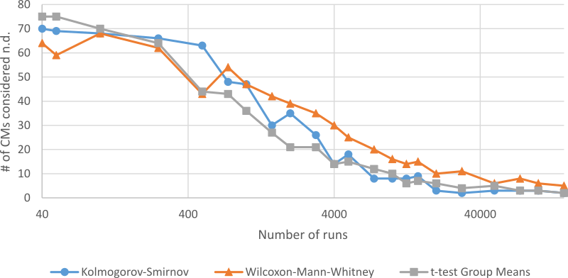
To test the sensitivity of the comparison, the meta-simulation generated run-lengths from 40 to 150,000. At the lowest run-length, 40, the meta-simulation ran the hypothetical “true” CVT model (“50000”) through 40 games, generating 40 data-points. It did the same for the plausible CMs, generating 40 data-points for each. The results are summarized in Figure 5 (see the Appendix for supplementary material). Practically all models are considered not different at 40 runs, between 60% and 76% at 750 runs, and less than 10% at 50,000 runs. Finally, at 150,000 runs, only between two to five of the models were still considered not different from the target true model. As an example, the 150,000 run-length is detailed in Table 3. An agreement between all three tests would indicate a high level of reliability compared to a single test. At this level the only simulation model that is accepted by all three tests is “50000”—the “true” CVT. However, even the two most powerful tests, in this case the K-S and t-test, both accepted other models as well as the true model.
| Model | K-S | W-M-W | t-test | Model | K-S | W-M-W | t-test |
| 50000 | n.d. | n.d. | n.d. | 20120 | diff. | n.d. | diff. |
| 40010 | n.d. | n.d. | diff. | 13001 | diff. | n.d. | diff. |
| 30020 | diff. | n.d. | diff. | 00320 | diff. | diff. | n.d. |
It can be argued that the high number of matching models highlights the closeness of the models. On the one hand, if we agree that the models were in fact too close, Experiment 1 shows that the way to prevent the closeness of the models from dominating the matching process would be to increase the power of the test (e.g., increase the number of data points). On the other hand, we could constrain the meta-simulation to only compare drastically different plausible CMs. But that would sidestep the issue—the proliferation of many similar models as a result of compounding (minor) reasonable assumptions. It should be noted that these models differed in fundamental assumptions about the participant’s behavior, and even at unusually high numbers of runs, many plausible models were considered equifinal.
Experiment 2: The stability of the CM output match
Experiment 2 investigates the stability of Experiment l’s results. Unlike systems dynamics and similar deterministic methods, our agent’s decision strategies are stochastic and consequently the simulation's output is stochastic. Statistics, as used by operations research, are designed to take a sample of the stochastic output and infer the nature of the simulation’s model. As social simulation researchers, we often take the output of a run with multiple data points and present that output as the simulation's true output (or close enough to be the true output). Experiment 2 asks the question, what effect does randomness have on our conclusions of internal validity? Do we believe our simulation, or should we run again just in case?
Experiment 2 took six run-lengths, 500, 1000, 2000, 3000, 4000, 5000, and recorded how often each model is considered “not different” if we replicated it 999 times again. Table 4 shows how many models were considered not different 100 percent of the time, between 90 and a 100 percent of the time, down to 0 percent of the time.
| x% of the time | # of Runs | |||||
| 500 | 1000 | 2000 | 3000 | 4000 | 5000 | |
| 100% | 0 | 0 | 0 | 0 | 0 | 0 |
| 90-99% | 35 | 16 | 9 | 8 | 7 | 6 |
| 80-89% | 15 | 12 | 5 | 2 | 2 | 3 |
| 70-79% | 8 | 12 | 8 | 4 | 1 | 0 |
| 60-69% | 6 | 3 | 2 | 2 | 4 | 1 |
| 50-59% | 1 | 6 | 5 | 3 | 1 | 2 |
| 40-49% | 0 | 5 | 6 | 4 | 3 | 2 |
| 30-39% | 0 | 4 | 5 | 6 | 4 | 3 |
| 20-29% | 0 | 3 | 4 | 4 | 3 | 4 |
| 10-19% | 1 | 3 | 5 | 7 | 5 | 7 |
| 1-9% | 3 | 1 | 10 | 9 | 11 | 9 |
| 0% | 2 | 6 | 12 | 22 | 30 | 34 |
The results demonstrate that as the number of runs increase, the number of models stable at 10 percent or lower increases and the number stable at 90 percent or above decreases. This is to be expected as statistical power increases with the number of runs. More importantly, no model was ever “not different” 100 percent of the time. Further, a large number of models remain in the 10–90% range.
Experiment 3: How long before declaring a model doesn’t fit?
Experiment 3 takes a longitudinal approach to the issue explored in Experiment 2. Experiment 2 suggested that if the researcher’s particular CM was rejected, run it again and it might be considered not different next time. Experiment 3 asks, if the simulation were run again, how many of the models previously considered different would now be considered not different?
We used the same simulations and methods as Experiments 1 and 2, but in Experiment 3 we focused on a conservative run-length of 2000 (2000 complete games). The meta-simulation performed 2000 runs for each model and recorded which models were considered not different from the true model (out of the 71 viable models). It then performed another 1999 replications and recorded when a new unique model was considered not different from the true model. Figure 6 presents the cumulative total number of models considered not different from the true model at least once in the previous runs.
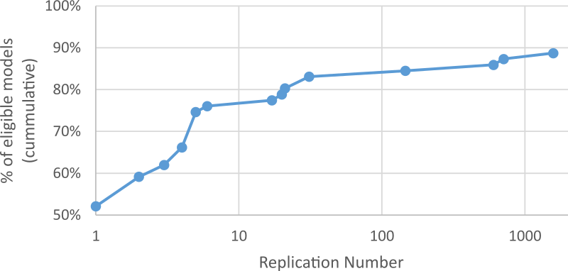
Experiment 1’s results show that at the 2000 game level, the K-S test found that 35 models, 49% of the total viable models, were considered not different from the true model. In contrast, Experiment 3 found 37 models eligible, 52% of the total. As the meta-simulation performed more replications, the number of unique models accepted rose, until replication number 1580 where the 63rd unique model is accepted at least once. Interestingly, relative stability was reached at the 31st replication, after which only 4 new models were accepted at the cost of 1969 replications.
Experiment 4: Reliability across run-lengths
A match result can be considered unreliable if there is a high probability that the results would change given another replication. Experiment 4 asks the question, how many times should we run the simulation before we’re confident that the results won’t shift with another run? Experiment 4 used the methods of Experiment 3 with run-lengths ranging from 40 to 150000.
Figure 7 shows that when the number of runs are low, from 40 to 1000, almost every model is accepted at least once, although it sometimes takes as many as 1623 replications, as found at the 750 run-length. This indicates the low reliability of low run-lengths. Only when we reach 10,000 runs are less than half of the models accepted.
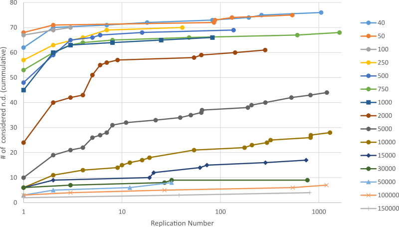
The results suggest that reliability requires a much larger run-length than Experiment 1 indicated. For example, Experiment 1 showed the K-S test accepted less than 10 models at 7500 runs, but Experiment 4 demonstrated that we need 30000 runs before the K-S test accepts a cumulative total of only 10 models. At 30000 runs, the stability of 9 models is reached after 32 replications, indicating this run-length is relatively stable.
General Discussion
Computational modeling aids theory-building because a computational model (CM) allows theorists to explore the dynamic consequences of their cognitive/verbal theory (CVT). It also aids communication by turning abstract concepts into specific concrete examples. In this paper we have used these benefits of computational modeling to illustrate that these are also its disadvantages. The theoretical argument and meta-simulation results indicate that computational modeling is a double-edged sword.
We described the computational modeling process as a Plan-Do-Check-Act cycle (Figure 2). We argued that the Do phase of the cycle presents the researcher with decision points—choices that are not theoretically significant enough to be driven by the researcher’s CVT, and not technically significant enough to be reflected in the researcher’s documentation or research reports. The researcher solves these decision points by making reasonable assumptions, such as choosing a float type instead of an int. We used a decision-tree analogy to understand the compound effects of making these reasonable assumptions (Figure 3). Since each decision point could result in two or more equally reasonable assumptions, each decision point results in at least two (and usually more) plausible CMs. Much like the many worlds interpretation of quantum mechanics, each reasonable assumption increases the total number of plausible CMs (Figure 3). Thus, the problem is that as the number of plausible CMs multiply, many other CMs could have become equally plausible models of that original CVT. The researcher believes that her one unique CM is the model of her CVT. But in truth, many of the other plausible CMs could also be considered the model of her CVT. These are the problems of reasonable assumptions leading to equifinality.
As a concrete example of our theoretical argument, we used a simple group decision-making task: five individuals choosing numbers to reach a goal with no communication. We proposed that a significant change in the model’s construction (the decision-making strategy of one of the agents) would be a conservative approximation of a researcher making a reasonable assumption during the CM construction phase. For example, where a researcher might choose to hold a variable in an int instead of a float, we chose to use a “Memory” agent instead of a “Random” agent. Our exponential number of plausible CMs (Figure 4) was an illustration of the computational researcher’s unrealized range of plausible CMs. We used one of these models as the hypothetical “true” CVT, and asked the question: how many of these reasonable CMs would we consider the same as the “true” CVT?
Experiment 1 demonstrated that when comparing a set of alternative models, at sample levels common in the literature, 98.6% of the alternative models are found to be “not different” from the target. It is entirely possible that, through no fault of the researcher, one CM simulated and compared to a target is just as acceptable as many other alternative models. This is particularly true if a low number of data points are generated. For example, Experiment 1 demonstrates that at 1000 data points or below there was a 50% chance that a randomly picked model would be considered not different. Only when we reach 15,000 to 50,000 runs do we declare less than 10% of the CMs “not different.” Experiments 2, 3 and 4 extend these findings by demonstrating that a model initially considered different may be considered not different if the simulation is run again. For example, Experiment 2 shows that even with 5000 runs, 37 models are found not different at least once, compared to the initial 18 in Experiment 1. Experiments 3 and 4 indicate that a researcher may need to simulate up to 150,000 data points before she can be sure that the chosen CM is in fact a good match to a hypothetical target system. These results may remind readers of the core problems of simulation validation, but the implications extend beyond the basic issue of statistical validation. These implications are explored in the following sections.
The dangers of using computational modeling to build theory
Cognitive verbal theories (CVTs) are by definition underspecified compared to the computational model (CM). Perhaps, as one reviewer noted, once the researcher begins translating the CVT into the CM, the CVT becomes obsolete. Does it even matter that the CM does not match the CVT? Maybe it does not matter what the CVT used to be, but only what the CM actually is. Alternatively, if the researcher is the one who translated her own CVT into a CM, who could doubt that the CM is the correct instantiation of that original CVT?
These are reasonable questions to ask, and there are two answers that help resolve them. First, consider the PDCA process of translating an initial CVT into a CM (Figure 2). Perhaps after starting to build the CM the researcher makes changes and assumptions that diverge from the original CVT. This is the DO stage of the translation process. After making those changes the researcher experiments and sees what the CM does, if and how it works, and learns from those assumptions (the Check stage). The researcher takes that knowledge and makes changes to her understanding of the system she is building (the Act stage), and plans the next incremental step in the translation process (the Plan stage). In short, the PDCA model describes how the researcher’s cognitive model of the system under study (the CVT) changes as the CM is built. In fact, the CVT is always the mental model of the researcher’s CM. The CVT is the researcher’s belief about what the system is doing, which is realized by the CM.
Second, and most importantly, unanticipated reasonable assumptions create a mismatch between what the researcher thinks she has created (the CVT) and what she has actually created (the CM). One may ask: shouldn’t it only matter what the CM actually is, since that is what the researcher is using to experiment on and learn from? In a way, yes. The experiments and results (measures) are happening with the CM as it actually is. However, as in all science, it is not the measure’s numbers that matter, it is the researcher’s interpretation of what those measurements mean. Suppose the researcher has a thermometer reading 102°C at sea level and thinks she has measured the boiling point of water, when actually she has measured the boiling point of a mixture of water and salt. This is the problem with reasonable assumptions—the researcher thinks she has simulated water, but she has actually built salt water.
Although these are relatively straightforward problems, the evidence from top-level journals indicates this is an important issue that needs to be better understood and addressed. For instance, one publication argued that reproducing a time series that looks like the time series of a real-world experiment participant, means this “demonstrates that the model is capable of describing [the effect under study]” (Vancouver et al. 2014 p. 64), and that “our theoretical model is capable of reproducing [the effect under study]” (Vancouver et al. 2010 p. 997). Of course, Vancouver and colleagues were not claiming that the model’s ability to produce similar output was a complete validation; the qualitative comparison was the first step, an existence proof showing that their CM (and by implication their CVT) could “account for the phenomena the model claims to explain” (Vancouver et al. 2014 p. 65). The CM (and CVT) then become a “possible explanation” for the system they model (Vancouver et al. 2014 p. 66).
However, therein lies the danger of equifinality and reasonable assumptions. Our meta-simulation results demonstrate that for every final simulation, there may be many other equally reasonable, statistically equivalent models with basic technical and theoretical differences. Even with this paper’s deliberately straightforward simulation, with only five agent types, and a target known with complete information, the meta-simulation showed it is difficult to reliably differentiate between candidate models. Practically speaking, if we choose a single operationalization after making many reasonable assumptions, what does it mean that our CM “works”? Does that mean our CVT works as well? If our CM demonstrates certain dynamics or emergent properties, does that mean our CVT does as well? Fundamentally, what can we learn about our CVT if our CM is one of many that could also have been made?
The results of our meta-simulation lead us to conclude that CMs cannot help us learn about our CVTs, because we cannot be sure they actually model our CVTs. Instead, we believe the benefit of computational modelling lies in the PDCA process itself.
The benefits of using computational modeling to build theory
Computational modeling (CM) and real-world experiments aid theory development in similar ways. To understand this parallel we should first describe the full Bavelas experiment. The experimental situation we modelled above was a simple condition: an experimental task of hitting target 17, 5 as the number of people, and no communication among them. Bavelas was investigating the broader theoretical issue of the effect of information on group decision-making. More specifically, his question was: will accurate information improve group decision making? Thus, the other important condition was when the group received accurate feedback of how far away the group total was from 17. For example, if the sum was 19, then the group was told that their sum was 2 over the target.
What kind of cognitive/verbal theory do we use to predict participant behavior? One line of thinking could be that accurate information will improve the group performance. After all, we have heard that information is good, and the idea of a “well informed decision” is practically a truism of modern business. Let the initial verbal theory be that accurate information will improve the group’s decision making. In fact, when participants were asked which of the two conditions (with or without feedback) will perform better, they selected the feedback condition. It may be that they had the same preconceptions as the researcher. It turns out that in the actual experiment the results are opposite of this verbal theory. That is, the group with no feedback outperforms the group with accurate feedback. The reason is that the group with feedback tries to use the feedback information, ends up constructing theories about how others might behave, and ends up with choices that are often peculiar. For example, if the group is two over the target, a member may think that maybe at least three people will try to correct for this, so maybe I should correct for overcorrection, and ends up choosing 7 (their initial share of 3, plus 4 for correction). Of course, these theories are wrong and the result is wide range of numbers being selected by the group members. The group takes longer to hit the target, and when they do there is no learning.
There is a quite a bit of thinking involved in order to go from the verbal theory to a concrete situation in which 5 people select a number to sum up to 17. This process of thinking is the art of doing research. It is very difficult to teach, and it is not included in the Vancouver and Weinhardt (Vancouver 2012) idea of verbal theory. If the verbal theory is that accurate feedback information improves decision making, the question is how does this get translated into a CM? The answer is that it can’t be directly translated because it is too underspecified. The abstract concepts need to be much more concrete before the translation process can begin.
One way to accomplish this transformation is by using thought experiments. Thought experiments are mental simulations of possible situations which are representative of the essential properties of the theory. We use our imagination to simulate concrete situations all the time. For example, what are the consequences of being late to a meeting? We have a mental model of the meeting which includes the participants, the social/cultural structure of the meeting, and we ask the question: what if I am late? We get an answer such as: I will look bad in front of my boss. We can’t mentally simulate conditions which are expressed in abstract language, such as: feedback information will improve group decision-making. This needs to be transformed into a concrete situation so a thought experiment or mental simulation can take place. Bavelas cleverly transformed this abstraction into a simple concrete situation of adding numbers chosen by the members to hit a target. It would be a guess on our part as to how he arrived at this concrete situation. But he must have considered a variety of examples and valued the simplicity of the situation, both for thinking/mental simulation and for experimentation. The point is that the path from verbal theory requires transformation to the concrete situations which represent them. These concrete situations can then be further explored either by experiments or by computational models.
This brings us to the benefit of CM for theory development. During the research process, experiments force us to operationalize abstract concepts into concrete measures. Likewise, computational models force us to define concepts at a programmable level which we may, otherwise, not do. For example, we may consider the concept of randomness as a decision mode for a participant. We may choose “random choice” as an explanation of behavior without further questioning. However, when the researcher tries to program randomness, he may note that he uses a complex mathematical formula coded into a built-in function (a pseudo-random number generator), as opposed to a simple “random choice” rule. This may raise the question: do we have a random generating function in our minds? Of course, we don’t have such a capability; our idea of randomness is dodging patterns, which raises the question of how randomness should be specified in a CM. If we wanted to code the human behavior of pattern-dodging, we would likely use propensity scores or randomness with weighting. But we cannot simply code “does not (usually) like to choose 3 more than twice in a row.” We would have to be specific by, e.g., specifying the exact proportional chance to select 3 or 4. Which proportion between 0.0 and 1.0 do we choose? How does that proportion change if the first choice was 3? Is the proportion the same for every participant? The point is: that during the process of constructing a CM, a fundamental question about the human perception of randomness has been raised. It isn’t that such questions could not be raised without CM construction, but rather that the process of CM construction makes it more likely. In the verbal theory mode, the researcher might be quite comfortable with the idea of random choice as an explanation.
It is worth pointing out that the problems of equifinality and reasonable assumptions also exist when the researcher examines her theory against reality. For example, the particular experiment could have been designed differently or relevant variable could have been defined and measured differently. That is, they are based on “reasonable assumptions” on the part of the researcher which are not usually discussed. For example, these days most papers do not include their exact instructions to the participants in their experiments, perhaps it is considered as a waste of space. Further, it is often not clear whether the same experiment can be replicated or not. In fact, when such an effort is made many studies cannot be replicated (Collaboration 2015). Most researchers do not test their operationalization with the kind of rigor we exposed our models too. The point is that the methodological issues raised here also apply to testing theories against the real world.
Practical Implications
We do not wish this work to be seen as an attack on computational modeling for theory-building. Far from it; we adore the methodology and firmly believe in its benefits: the iterative process of model building and theory construction described by Harrison et al. (Harrison et al 2007) and in our PDCA model (Figure 2), and the benefits of working through the implications of dynamic theories (Vancouver & Weinhardt 2012; Weinhardt & Vancouver 2012). But the findings here demonstrate in concrete terms the practical issues facing computational researchers.
We propose two practical recommendations based on this study. First, it is difficult to prove that the conceptual model is accurately programmed into the computational model. Just as computer scientists have recognized that the only accurate design document is the code itself (Reeves 1992, 2005), simulation researchers should realize that the code is the only accurate description of their CM. Even a complete set of model parameters and instructions may be inaccurate. The only way of disseminating what was actually modelled is to open source the model’s code so that it can be run, investigated, and improved upon. At this time, only a few journals strongly recommend the sharing of simulation code (e.g., JASSS), and as far as we know none absolutely require it. Computational models should be released in code so that readers can see every reasonable assumption, whether intentional or accidental. As shown in the experiments above, the actual coded model may be quite different from the CM the researcher presented in the published paper. Importantly, it is likely that there is no malicious intent in the difference. Honest researchers are not trying to pull a fast one on the readers by using a computation model with fundamental differences from the published model. The difference is simply because the printed page and our cognitive/verbal models lack the specificity of computational model’s code. That is the fundamental problem, after all.
Second, we need an easier method of tracking the exponential tree of reasonable assumptions diagrammed in Figure 3 and Figure 4 and tools to perform sensitivity analysis. The easiest type of sensitivity analysis is performed on the numerical parameters to test for robustness during the validation stage (admirably conducted by Vancouver et al. 2010, 2014). A far more difficult, but far more useful, sensitivity analysis can be performed on the theoretical and technical assumptions made in development stage itself (the Do stage in the PDCA model). To our knowledge, a sensitivity analysis on the structure of a set of plausible CMs has never been done before, and would require new tools. For example, such a meta-sensitivity analysis would test more than simply differences in initial conditions or variable ranges. Instead, the differences would be at the level of how the program is structured (e.g., different logistic functions for making a decision), the types used (e.g., int vs float), and other structural choices that are not included in traditional sensitivity analysis tooling (e.g., different object models, or even object vs functional designs). This structural sensitivity analysis could be significant benefit for theory-building. It will strengthen the researcher’s faith that the CM driving the theory development actually represents the original CVT, assumption by reasonable assumption.
In summary, we contend that the problems are subtle, and not technical at all. The meta-simulation results show that all computational models beg the question: Are we certain that this one computational model represents our conceptual theory? And what about all the others? As simulation researchers, we need to address these questions before we can claim the output of our simulations tell us anything about the theories they are proposed to represent.
Notes
- A healthy debate has consumed philosophers of economics about whether or not this is good for economics (Musgrave 1981). Despite this, all agree that a startlingly accurate model need not have any connection to the reality it predicts.
- Assuming an explanatory model is given the information it requires, it should be able to predict what it explains. In practice, of course, explanatory models are often not given the information they need ahead of time to predict future events (e.g., theories of earthquakes, many explanatory macroeconomic or political models, etc.). It is only after the event, and all the required information is provided, that these explanatory models give the correct prediction. Conversely, if they did not, they would probably not be considered very accurate explanations.
- The model is publicly available at: https://www.openabm.org/model/5043/version/1.
- We were limited to one Corrector (Co) agent. If there were two, they would endlessly loop. E.g., corrector A would predict what corrector B would choose, but B’s choice depends on predicting what A would choose, and so on.
Appendix
Supporting Tables
| # of Runs | Kolmogorov-Smirnov | Wilcoxon-Mann-Whitney | t-test Group Means | ||||||
| n.d. | Tot | % | n.d. | Tot | % | n.d. | Tot | % | |
| 40 | 70 | 71 | 0.99 | 64 | 71 | 0.90 | 75 | 79 | 0.95 |
| 50 | 69 | 71 | 0.97 | 59 | 71 | 0.83 | 75 | 76 | 0.99 |
| 100 | 68 | 71 | 0.96 | 68 | 71 | 0.96 | 70 | 74 | 0.95 |
| 250 | 66 | 71 | 0.93 | 62 | 71 | 0.87 | 64 | 71 | 0.90 |
| 500 | 63 | 71 | 0.89 | 43 | 71 | 0.61 | 44 | 71 | 0.62 |
| 750 | 48 | 71 | 0.68 | 54 | 71 | 0.76 | 43 | 71 | 0.61 |
| 1000 | 47 | 71 | 0.66 | 47 | 71 | 0.66 | 36 | 71 | 0.51 |
| 1500 | 30 | 71 | 0.42 | 42 | 71 | 0.59 | 27 | 71 | 0.38 |
| 2000 | 35 | 71 | 0.49 | 39 | 71 | 0.55 | 21 | 71 | 0.30 |
| 3000 | 26 | 71 | 0.37 | 35 | 71 | 0.49 | 21 | 71 | 0.30 |
| 4000 | 14 | 71 | 0.20 | 30 | 71 | 0.42 | 14 | 71 | 0.20 |
| 5000 | 18 | 71 | 0.25 | 25 | 71 | 0.35 | 15 | 71 | 0.21 |
| 7500 | 8 | 71 | 0.11 | 20 | 71 | 0.28 | 12 | 71 | 0.17 |
| 10000 | 8 | 71 | 0.11 | 16 | 71 | 0.23 | 10 | 71 | 0.14 |
| 12500 | 8 | 71 | 0.11 | 14 | 71 | 0.20 | 6 | 71 | 0.08 |
| 15000 | 9 | 71 | 0.13 | 15 | 71 | 0.21 | 7 | 71 | 0.10 |
| 20000 | 3 | 71 | 0.04 | 10 | 71 | 0.14 | 6 | 71 | 0.08 |
| 30000 | 2 | 71 | 0.03 | 11 | 71 | 0.16 | 4 | 71 | 0.06 |
| 50000 | 3 | 71 | 0.04 | 6 | 71 | 0.08 | 5 | 71 | 0.07 |
| 75000 | 3 | 71 | 0.04 | 8 | 71 | 0.11 | 3 | 71 | 0.04 |
| 100000 | 3 | 71 | 0.04 | 6 | 71 | 0.08 | 3 | 71 | 0.04 |
| 150000 | 2 | 71 | 0.03 | 5 | 71 | 0.07 | 2 | 71 | 0.03 |
| Rep. # | # of Models | Cummulative total | % of Eligible Models |
| 1 | 37 | 37 | 52% |
| 2 | 5 | 42 | 59% |
| 3 | 2 | 44 | 62% |
| 4 | 3 | 47 | 66% |
| 5 | 6 | 53 | 75% |
| 6 | 1 | 54 | 76% |
| 17 | 1 | 55 | 77% |
| 20 | 1 | 56 | 79% |
| 21 | 1 | 57 | 80% |
| 31 | 2 | 59 | 83% |
| 146 | 1 | 60 | 85% |
| 604 | 1 | 61 | 86% |
| 710 | 1 | 62 | 87% |
| 1580 | 1 | 63 | 89% |
| Number of Runs | |||||||||
| 40 | 50 | 100 | 250 | 500 | |||||
| Run | Models | Run | Models | Run | Models | Run | Models | Run | Models |
| 1 | 62 | 1 | 68 | 1 | 67 | 1 | 57 | 1 | 48 |
| 2 | 8 | 2 | 3 | 2 | 2 | 2 | 6 | 2 | 11 |
| 7 | 1 | 86 | 1 | 3 | 1 | 4 | 3 | 3 | 6 |
| 18 | 1 | 88 | 1 | 7 | 3 | 5 | 1 | ||
| 83 | 1 | 131 | 1 | 41 | 1 | 6 | 1 | ||
| 194 | 1 | 537 | 1 | 16 | 1 | ||||
| 262 | 1 | 136 | 1 | ||||||
| 1056 | 1 | ||||||||
| Total | 76 | Total | 75 | Total | 70 | Total | 70 | Total | 69 |
| 750 | 1000 | 2000 | 5000 | 10000 | |||||
| Run | Models | Run | Models | Run | Models | Run | Models | Run | Models |
| 1 | 53 | 1 | 45 | 1 | 24 | 1 | 10 | 1 | 6 |
| 2 | 7 | 2 | 15 | 2 | 16 | 2 | 9 | 2 | 5 |
| 3 | 3 | 3 | 3 | 3 | 2 | 3 | 2 | 4 | 2 |
| 4 | 1 | 8 | 1 | 4 | 1 | 4 | 1 | 9 | 1 |
| 8 | 1 | 25 | 1 | 5 | 8 | 5 | 4 | 10 | 1 |
| 48 | 1 | 83 | 1 | 6 | 4 | 6 | 1 | 12 | 1 |
| 605 | 1 | 7 | 1 | 7 | 1 | 16 | 1 | ||
| 1623 | 1 | 9 | 1 | 8 | 3 | 19 | 1 | ||
| 54 | 1 | 11 | 1 | 54 | 3 | ||||
| 64 | 1 | 22 | 1 | 176 | 1 | ||||
| 141 | 1 | 39 | 1 | 209 | 1 | ||||
| 285 | 1 | 50 | 1 | 297 | 1 | ||||
| 64 | 1 | 323 | 1 | ||||||
| 65 | 1 | 824 | 1 | ||||||
| 190 | 1 | 830 | 1 | ||||||
| 207 | 1 | 1300 | 1 | ||||||
| 286 | 1 | ||||||||
| 526 | 2 | ||||||||
| 822 | 1 | ||||||||
| 1206 | 1 | ||||||||
| Total | 68 | Total | 66 | Total | 61 | Total | 44 | Total | 28 |
| 15000 | 30000 | 50000 | 100000 | 150000 | |||||
| Run | Models | Run | Models | Run | Models | Run | Models | Run | Models |
| 1 | 6 | 1 | 6 | 1 | 3 | 1 | 3 | 1 | 2 |
| 2 | 3 | 3 | 1 | 2 | 2 | 3 | 1 | 38 | 1 |
| 19 | 1 | 27 | 1 | 12 | 1 | 27 | 1 | 808 | 1 |
| 21 | 2 | 32 | 1 | 32 | 2 | 544 | 1 | ||
| 62 | 2 | 765 | 1 | 1199 | 1 | ||||
| 73 | 1 | ||||||||
| 287 | 1 | ||||||||
| 743 | 1 | ||||||||
| Total | 17 | Total | 9 | Total | 9 | Total | 7 | Total | 4 |
Details about the use of the t tests in the model comparisons
Note that the t-test compares group means, so the total number of runs were split into trials, such that the total number of games (runs multiplied by trials) was equal to total runs used in the non-parametric tests. All comparisons were at the 0.05 level of significance.
The t-test used the following runs: 10, 10, 10, 10, 25, 25, 25, 25, 25, 25, 50, 50, 50, 50, 50, 50, 100, 100, 100, 100, 200, and 200, respectively paired with the following trial numbers: 4, 5, 10, 25, 20, 30, 40, 60, 80, 120, 80, 100, 150, 200, 250, 300, 200, 300, 500, 750, 500, and 750.
References
AXTELL, R., Axelrod, R., Epstein, J. M., & Cohen, M. D. (1996). Aligning simulation models: A case study and results. Computational and Mathematical Organization Theory,1(2), 123–141. [doi:10.1007/BF01299065]
BALCI, O. (1998). Verification, validation, and testing. In J. Banks (Ed.), Handbook of Simulation (Vol. 10, pp. 335–393). New York, NY: John Wiley and Sons. [doi:10.1002/9780470172445.ch10]
BANKS, J., Carson, J. S., & Nelson, B. L. (1996). Discrete event system simulation (2nd Ed). Upper Saddle River, NJ: Prentice hall.
BONABEAU, E. (2002). Agent-based modeling: methods and techniques for simulating human systems. Proceedings of the National Academy of Sciences of the United States of America, 99 Suppl 3, 7280–7. [doi:10.1073/pnas.082080899]
COLLABORATION, O. S. (2015). Estimating the reproducibility of psychological science. Science, 349(6251), aac4716. [doi:10.1126/science.aac4716]
DAVIS, J. P., Eisenhardt, K. M., & Bingham, C. B. (2007). Developing theory through simulation methods. Academy of Management Review, 32(2), 480–499. [doi:10.5465/AMR.2007.24351453]
EPSTEIN, J. M. (1999). Agent-based computational models and generative social science. Complexity, 4(5), 41–60. [doi:10.1002/(SICI)1099-0526(199905/06)4:5<41::AID-CPLX9>3.0.CO;2-F]
FISS, P. C. (2007). A set-theoretic approach to organizational configurations. Academy of Management Review, 32(4), 1180–1198. [doi:10.5465/AMR.2007.26586092]
FRIEDMAN, M. (1953). Essays in positive economics. Chicago, IL: University of Chicago Press.
GOLDBERG, D. (1991). What every computer scientist should know about floating-point arithmetic. ACM Computing Surveys, 23(1), 5–48. [doi:10.1145/103162.103163]
GRESOV, C., & Drazin, R. (1997). Equifinality: Functional equivalence in organization design. Academy of Management Review, 22(2), 403–428.
GRUNE-YANOFF, T., & Weirich, P. (2010). The Philosophy and Epistemology of Simulation: A Review. Simulation & Gaming, 41(1), 20–50. [doi:10.1177/1046878109353470]
HAAHR, M. (2016). Random.org: True Random Number Service. Retrieved March 18, 2016, from http://www.random.org
HARRISON, J. R., Lin, Z., Carroll, G. R., & Carley, K. M. (2007). Simulation modeling in organizational and management research. Academy of Management Review, 32(4), 1229–1245. [doi:10.5465/AMR.2007.26586485]
HASSAN, S., Arroyo, J., Galán, J. M., Antunes, L., & Pavón, J. (2013). Asking the oracle: Introducing forecasting principles into agent-based modelling. Journal of Artificial Societies and Social Simulation, 16(3), 13: https://www.jasss.org/16/3/13.html. [doi:10.18564/jasss.2241]
HOFMANN, M. (2013). Simulation-based exploratory data generation and analysis (data farming): a critical reflection on its validity and methodology. The Journal of Defense Modeling and Simulation: Applications, Methodology, Technology, 10(4), 381–393. [doi:10.1177/1548512912472941]
KATZ, D., & Kahn, R. L. (1978). The social psychology of organizations (2d ed.). New York: Wiley.
LANDRY, M., Malouin, J.-L., & Oral, M. (1983). Model validation in operations research. European Journal of Operational Research, 14(3), 207–220. [doi:10.1016/0377-2217(83)90257-6]
LAW, A. M., & Kelton, W. D. (2000). Simulation modeling and analysis (3rd Ed, Vol. sp). Boston, MA: McGraw-Hill.
LEVITT, R. E. (2004). Computational Modeling of Organizations Comes of Age. Computational & Mathematical Organization Theory, 10(2), 127–145. [doi:10.1023/B:CMOT.0000039166.53683.d0]
MIHRAM, G. A. (1972). Some practical aspects of the verification and validation of simulation models. Operational Research Quarterly, 23(1), 17–29. [doi:10.1057/jors.1972.3]
MOEN, R. D., & Norman, C. L. (2010). Circling Back. Quality Progress, 43(11), 22–28.
MUSGRAVE, A. (1981) "Unreal assumptions" in economic theory: The F-Twist untwisted. Kyklos, 34(3), 377–387.. [doi:10.1111/j.1467-6435.1981.tb01195.x]
NORTON, J. (1991). Thought Experiments in Einstein’s Work. In T. Horowitz & G. J. Massey (Eds.), Thought Experiments In Science and Philosophy (pp. 129–144). Savage, MD: Rowman and Littlefield.
O’REILLY, K., Paper, D., & Marx, S. (2012). Demystifying Grounded Theory for Business Research. Organizational Research Methods, 15(2), 247–262. [doi:10.1177/1094428111434559]
ORESKES, N., Shrader-Frechette, K., & Belitz, K. (1994). Verification, validation, and confirmation of numerical models in the earth sciences. Science, 263(5147), 641–646. [doi:10.1126/science.263.5147.641]
REEVES, J. W. (1992). What is software design. C++ Journal, 2(2), 12–14.
REEVES, J. W. (2005). What Is Software Design: 13 Years Later. Developer.* Magazine, 23.
SCHÖNER, G. (2008). Dynamical systems approaches to cognition. In R. Sun (Ed.), Cambridge handbook of computational cognitive modeling (pp. 101–126). Cambridge, UK: Cambridge University Press. [doi:10.1017/cbo9780511816772.007]
TABER, C. S., & Timpone, R. J. (1996). Computational modeling. Thousand Oaks, CA: Sage. [doi:10.4135/9781412983716]
VANCOUVER, J. B., & WEINHARDT, J. M. (2012). Modeling the Mind and the Milieu: Computational Modeling for Micro-Level Organizational Researchers. Organizational Research Methods, 15(4), 602–623. [doi:10.1177/1094428112449655]
VANCOUVER, J. B., Weinhardt, J. M., & Schmidt, A. M. (2010). A formal, computational theory of multiple-goal pursuit: integrating goal-choice and goal-striving processes. The Journal of Applied Psychology, 95(6), 985–1008. [doi:10.1037/a0020628]
VANCOUVER, J. B., Weinhardt, J. M., & Vigo, R. (2014). Change one can believe in: Adding learning to computational models of self-regulation. Organizational Behavior and Human Decision Processes, 124(1), 56–74. [doi:10.1016/j.obhdp.2013.12.002]
VON BERTALANFFY, L. (1968). General Systems Theory: Fundations, Development, Applications. New York, NY: George Braziller.
WEBB, B. (2001). Can robots make good models of biological behaviour? Behavioral and Brain Sciences, 24(06), 1033–1050. [doi:10.1017/s0140525x01000127]
WEINHARDT, J. M., & Vancouver, J. B. (2012). Computational models and organizational psychology: Opportunities abound. Organizational Psychology Review, 2(4), 267–292. [doi:10.1177/2041386612450455]
YILMAZ, L. (2006). Validation and verification of social processes within agent-based computational organization models. Computational and Mathematical Organization Theory, 12(4), 283–312. [doi:10.1007/s10588-006-8873-y]