
Introduction
Aberdeen City and suburbs are located in Northeast Scotland, and are home to more than 450,000 people. Largely due to the North Sea oil industry, Aberdeen City has one of the highest income and lowest unemployment rates in the UK (Aberdeen City Council 2015). The population in Aberdeen City and Shire increased by 10.2% and 11.0% respectively between 2004 and 2014, mostly due to net migration into the area. Aberdeenshire also has one of the highest car ownership rates in the country (Aberdeen City Council 2015). Rapid population growth has posed challenges to the existing transport network. For commuters, having to spend a long time driving in congested traffic can cause health problems (Strazdins & Loughrey 2008;Tranter 2010). Congestion also increases CO2 emissions, which is harmful to the environment.
This paper develops an agent-based model of the daily commute in Aberdeen City and the surrounding area. We set up the environment so that it represents the actual landscape and existing (principal) road network in the area using Geographic Information System (GIS) data. Agents representing commuters and employers reflect the geographic distribution of businesses and homes in the area. We simulate individual commuters in various social contexts that shape the daily commuting patterns in Aberdeen, such as a flexitime arrangement, the level of urban concentration, the construction of a bypass and the existence of cyclists, exploring their impact on commute time, commute time reliability, and CO2 emission. Finally, we discuss how we can design social policies and infrastructure to achieve a more desirable outcome.
We find that flexitime will significantly reduce total CO2 emissions from traffic. It also reduces peak CO2 concentration. However, reduction in CO2 emissions declines more slowly as more flexitime is introduced. Flexitime reduces commute time length and variability, and hence has a larger time-saving effect than previously understood. We find that although higher urban concentration will increase the level of congestion in urban areas, overall it will reduce mean commuting time and total CO2 emissions from traffic because people living in urban areas drive less on average and are more likely to walk or cycle. We find that the new bypass will slightly reduce mean commute time, but slightly increase total CO2 emissions, due to higher speeds and longer overall travel distances. Finally we find that, contrary to the complaint that drivers are slowed down by cyclists, having cyclists on the road does not lead to longer commute times or larger commute time variability.
The paper proceeds as follows. Section 2 reviews relevant literature. Section 3 presents the agent-based model using the ODD protocol. Section 4 discusses treatment factors, experiment design and model output. Section 5 presents the results and discussion. Section 6 validates model results. Section 7 concludes.
Approaches to Traffic Simulation and Travel-Related Decision Making
One approach to traffic simulation is traffic cellular automata (TCA) models, which are computer simulations of a large number of individual vehicles that form dynamic traffic flows. In TCA models, space is discretized into cells as small as 7.5 metres wide, and short time steps of around one second are used. Due to their flexibility and computational efficiency, TCA models are able to simulate realistic micro-level traffic flow, and reproduce common traffic flow patterns such as free flow, transition flow and congested flow (Lárraga et al. 2002;Maerivoet & De Moor 2005). Most TCA models use the car-following rule to model vehicle movement, where a vehicle follows the car in front of it while trying to maintain a safe distance. They also assume single lanes that disallow lane changing or overtaking (Lárraga et al. 2005; Wang et al. 2001), though some have modelled two-lane carriageways (Nagatani 1993). Traffic flow controls such as traffic lights and junctions are sometimes included as well (Benjamin et al. 1996; Simon & Nagel 1998).
Another approach is agent-based models (ABMs), which are computer simulations that explicitly represent multiple heterogeneous, interacting individuals operating in a common environment. Where agent-based models have a spatially-explicit cellular representation, they can be similar to cellular automata models. However, as Cioffi-Revilla and Gotts (2003) (paragraph 4.11) observe, spatially-explicit agent-based models that depart from fixed spatial neighbourhoods of interaction cannot be translated to cellular automata. Such increased flexibility of agent-based models enables researchers to explore more strategic behaviour while still representing emerging traffic flow patterns from individual vehicle behaviour.
Duijn et al. (2003) have argued that agent-based models can be used for policymaking on congestion and transport planning. Examples include Dia (2002)’s ABM of individual driver behaviour given real-time data collected in a behavioural survey in Brisbane, Australia. Klügl and Bazzan (2004)’s agent-based traffic simulation features agents with a heuristic adaptation model to choose the route. Ma et al. (2014) have an ABM of the road network in Shanghai that is used to analyse the impact of charging station location on electric vehicle adoption. Gargiulo et al. (2012) have an ABM with just one parameter, which simulates distributions of commuters. Malik et al. (2015) used ABM to investigate the impact of improved urban transportation on population density and creativity diffusion.
A branch of the transport literature has been looking at the route choice behaviour of drivers. Studies differ in their assumptions regarding rationality, information processing and heterogeneity of drivers. Classic equilibrium analyses of transportation systems are based on the assumption that drivers are rational, homogeneous, have perfect information and unlimited information processing capabilities ( Wardrop 1952). However, researchers have since modified these assumptions and explored alternative behavioural rules. Nakayama et al. (2001) countered the assumption of driver rationality, arguing that drivers use simple rules to choose routes, and are heterogeneous in their preferences and perceptions. Likewise, Ramming (2001) showed that drivers are habitual rather than using full information to choose a route to minimize distance or time. Arslan and Khisty (2006) use fuzzy ‘if-then’ rules to represent drivers’ route choice rules and preferences.
Drivers can also respond to new information, such as real-time or pre-trip travel time information. Mahmassani and Liu (1999) studied drivers’ route-switch decisions under advanced traveller information systems (ATIS) and concluded that drivers will only switch route if expected travel time reduction exceeds a certain threshold. Abdel-Aty and Abdalla (2006) conducted laboratory experiments with a travel simulator and found that remaining travel time and familiarity with the device are two factors significantly influencing route-switch response to ATIS. Adler (2001) uses laboratory experiments to investigate the effects of route guidance and traffic advice on route choice behaviour. With the exception of equilibrium analyses based on rational behaviour, most studies assume that changes in driver behaviour and route choice will not fundamentally shift the dynamics of the aggregate traffic system. However, the assumption is violated when a large number of drivers in the system respond to the new information and change routes simultaneously.
When making travel-related decisions, travellers do not only consider the length of travel time, but also its variability. Researchers have long recognized the importance of travel time reliability in travel-related decision making (Gaver Jr 1968; Jackson & Jucker 1982; Knight 1974). Travel time variability is regarded as a cost to travellers due to the additional risks or uncertainty it creates or a buffer-time selected by travellers. Reduction in variability rather than mean travel time is of higher value to travellers, with studies by Asensio and Matas (2008) of drivers in Barcelona and Batley and Ibáñez (2012) of rail passengers in the UK both finding that reduction in variability is valued more than twice as highly as mean; and Avineri and Prashker (2005) that sensitivity to variance in travel time is inversely related to that of duration. Bhat and Sardesai (2006) found that travel time reliability is an important variable in commute mode choice decision in Austin, USA. These findings motivated us to look at both commute time length and reliability as model outputs.
Finally, regarding the environmental impact of transport, Spangenberg and Lorek (2002) showed that transport is an area of individual consumption that has a large environmental impact. Road transport accounts for around a fifth of CO2 emissions in the EU (European Commission 2016), a quarter in the UK (Gov.UK 2016), and a third in the U.S (Barth & Boriboonsomsin 2008). Moreover, CO2 emissions are highly related with congestion and driving speed. Barth and Boriboonsomsin (2008) found that CO2 emissions can be reduced by up to almost 20% through congestion mitigation, speed management, and the elimination of the acceleration and deceleration process during congested conditions. In a case study in Portland, Figliozzi (2011) show that congestion has a significant impact on CO2 emissions from commercial vehicles. Therefore, any social policy and infrastructural design that improve traffic flow and reduce congestion will bring additional environmental benefits of reducing CO2 emissions.
The model
The model is developed in NetLogo (Tisue & Wilensky 2004). This section follows the Overview, Design concepts and Details (ODD) protocol to describe the model (Grimm et al. 2006; Grimm et al. 2010), omitting the input data section because it does not apply to our model, and the design concepts section.
Purpose
The purpose of the model is to analyse the impact of factors such as a flexitime workplace arrangement, the level of urban concentration, a new bypass, and cyclists sharing roads with cars on commute time and variance, and total CO2 emissions from traffic in Aberdeen City and Shire.
Agent Classes and Attributes
The agent classes (or turtles in Netlogo) in the model are commuters, cars, and bicycles. Commuters are people who live and work in the area. Each commuter has a specific home and work location. Commuters go to and from work every day at a chosen journey start time and by the chosen travel mode. Cars and bicycles are travelling agents on the roads. They are travelling at a speed and acceleration (negative if deceleration) that are determined by the local speed limit, and cars and bicycles in front of them. In the model, cars emit CO2 while bicycles don’t.
There are two main types of patch: road patches (which collectively form the road network) and non-road patches. There are six road types: A, A-trunk, B, minor, urban and urban-trunk, and each has a different speed limit. According to Department for Transport (2012), the A roads are major roads, the B roads are connecting roads, and trunk roads are roads with dual carriageways. All classes of road have a different speed limit in urban areas. Non-road patches are distinguished by the 8-fold Scottish Government Urban Rural Classification (The Scottish Government 2014), which classifies areas in Scotland based on population density and time to access services (Figure 2). Employers and residences are located on non-road patches. Table 1, Table 2 and Table 3 list the main attributes of commuter, car and patch agents respectively.
| Commuter Attribute | Description | Endogenous? | Dynamic? |
|---|---|---|---|
| Employer | Employer, work location | N | N |
| Car | Cars owned by the agent | N | N |
| Bicycles | Bicycles owned by the agent | N | N |
| Home | Home, home location | N | N |
| Travel mode | Walk, cycle or drive | Y | N |
| Journey start time | Time to set off for work | Y | Y |
| Route to work today | Chosen route to work for today | Y | Y |
| Route to home today | Chosen route to home for today | Y | Y |
| Journey time to work today | Journey time to work today | Y | Y |
| Journey time to home today | Journey time to home today | Y | Y |
| Journey time history | History of all past journey time | Y | Y |
| Congestion memory | Memory of past congestion on all roads | Y | Y |
| Car or Bicycle Attribute | Description | Endogenous? | Dynamic? |
|---|---|---|---|
| Owner | Owner of the car (who is a commuter) | N | N |
| Car ahead | The car ahead of it if any | Y | Y |
| Bicycle ahead | The bicycle ahead of it if any | Y | Y |
| Current speed | Current speed | Y | Y |
| Current acceleration | Current acceleration (negative if deceleration) | Y | Y |
| Current CO2 emission | Current instant CO2 emission | Y | Y |
| Patch Attribute | Description | Endogenous? | Dynamic? |
|---|---|---|---|
| Patch type | Road or non-road patch | N | N |
| Speed limit | Road patch only, speed limit on the patch | N | N |
| Urban rural classification | 8-fold urban rural classification (relevant for non-road patch only) | N | N |
| Postcode | Postal code of the patch (relevant for non-road patch only) | N | N |
Process Overview and Scheduling
Time is discrete in the model. Each time step represents 2.8 seconds in real time. Every morning, individual commuters set off for work by their transport mode (drive, walk, cycle) at a time of their choice, which depends on the flexitime range and the distance from home to work. In the same way, commuters drive home from work in the afternoon. The time they leave work depends on the time they arrive at work in the morning. Every morning and afternoon, cars are driving on roads to and from work. Each run consists of 60 consecutive days, with observations taken from the last 40. We choose 60 days so that the observed period is long enough to make inferences about the mean and variance of travel time. Moreover, we exclude the first 20 days as initial burn-out period during which agents accumulate memories and make adjustments accordingly. The scheduling of the model is as follows.
At the beginning of the simulation:
- agents decide their travel mode (sub-model, Section 3.5.1);
Every day:
- agents update their route choice (sub-model, Section 3.5.2),
- agents decide their journey start time (depends on flexitime range, a model parameter);
Every three seconds:
- commuters drive/cycle/walk on the road to work or from work (sub-model, Section 3.5.1),
- instant CO2 emissions are computed from cars on the road (sub-model, Section 3.5.4)
Initialization
The landscape and road network of Aberdeen City and Shire form the environment in which commuter agents drive and interact. We simulate the landscapes and road network using Ordnance Survey GIS data (Ordinance Survey 2015). The modelled area is 40×50 km and each patch represents a 100×100 m area. We also simulate a new bypass (the Aberdeen Western Peripheral Route – AWPR) that is currently under construction and expected to be completed in 2017 (Transport Scotland 2015a), which can be enabled or disabled as one of the treatment factors. However, controversies around the project have arisen since its inception, including the impact on local communities, and the actual benefit and cost of the project (Transport Scotland 2015b).
To simplify the simulation and avoid over-complication, the model does not have traffic flow controls such as traffic lights and roundabouts at junctions or elsewhere, nor does it represent one-way streets. Figure 1 shows the location of roads, homes and businesses in the area of study, with road types represented by different colours.
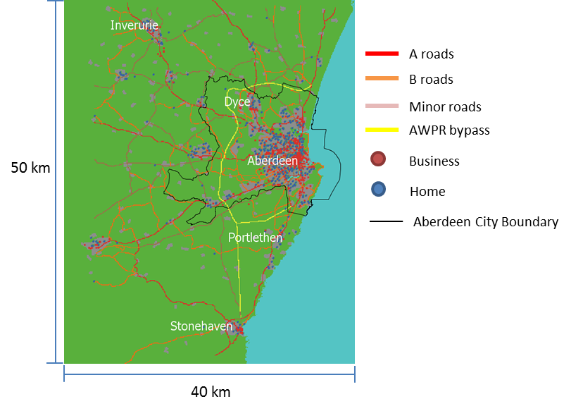
Each commuter is assigned a home and a work address using Ordnance Survey address data (Ordinance Survey 2015). Work addresses are found by identifying unique postcodes with a valid operation name such as “Aberdeenshire Council” or “Balmoral Group Ltd”. There are 718 work addresses identified in this way. On the other hand, home addresses are those that do not occupy a unique postcode and have no operation name. After identifying all home addresses in the data, a random sample is drawn, and each commuter is assigned a home address in the sample. As a result, the spatial distribution of homes and businesses in the model environment matches the actual geographic distribution in the area.
We do not know the relative size of the 718 identified employers in the area, and assume they are of the same size. Since a business already needs to be large enough to occupy a unique postcode to qualify as an employer in the model and, as can be seen in Figure 1, businesses are clustered spatially, we believe that the problem caused by assigning the same weight to each business can somewhat be alleviated. Another assumption made in the absence of appropriate data is the independence between a commuter’s work and home location. In reality, although people consider their workplace location when deciding where to live, other factors influence this choice, such as house quality and price, and school quality, which are beyond the scope of this study. The model may be seen as representing a worst-case scenario where people do not optimize the distance between home and work.
The Scottish Government Urban Rural Classification (The Scottish Government 2014) provides a consistent way of defining urban and rural areas across Scotland. We use the most recent (2013-2014) classification to identify urban and rural areas in Aberdeen City and Shire. The area of study is diverse in the level of urbanization, covering five out of eight urban-rural classifications (Figure 2).

The speed limits for the different types of roads in the model are consistent with current speed limits in the UK for various road types (Gov.UK 2015a), but do not necessarily correspond to those enforced locally. Vehicle acceleration is based on the “0-60 time” parameter for a typical family car, which measures the time it takes to accelerate from 0 to 60 mph. Deceleration is based on the typical braking distance at 60 mph (Gov.UK 2015b). The number of commuting agents is 1000. We choose to simulate 1000 agents so that it roughly represents the commuting population in the area (the commuting population in the area is roughly 100,000 according to the 2011 Census (ONS 2011), and the geographic scale is 1:100). For every parameter combination, we run 10 replications, each with a different random seed. Table 4 lists the initialization of model parameters.
| Parameter | Value/Distribution |
|---|---|
| 0-60 time | 12 seconds |
| Braking distance at 60 mph | 55 metres |
| Number of commuters | 1000 |
| Number of employers | 718 |
| Speed limit for A road | 60 mph |
| Speed limit for A trunk road | 70 mph |
| Speed limit for B road | 60 mph |
| Speed limit for minor road | 50 mph |
| Speed limit for urban road | 30 mph |
| Speed limit for urban trunk road | 40 mph |
| Speed of cycling | 12 mph |
| Speed of walking | 3 mph |
Sub-models
Travel Mode Allocation
The model has three transport modes: walking, cycling and driving. Although public transport is important, including all the bus routes in the area, each of which has different capacity, time tables and stops would be too complicated. Moreover, compared with larger cities such as Edinburgh, the use of public transport is lower in Aberdeen. Rail, the only other public transport option in the area, is also ignored.
We included walking and cycling so that we could analyse the effect of urban concentration, as people living in urban areas are more likely to walk or cycle to work. The allocation of travel mode among commuters is done in a probabilistic way. We assume that the probability a commuter would choose to walk or cycle is a decreasing function of commute time by that mode. We choose a simple probabilistic model (Figure 3) over more complicated ones typically used, such as the discrete choice model, because it’s not our purpose to study the role of individual characteristics in travel mode choice.
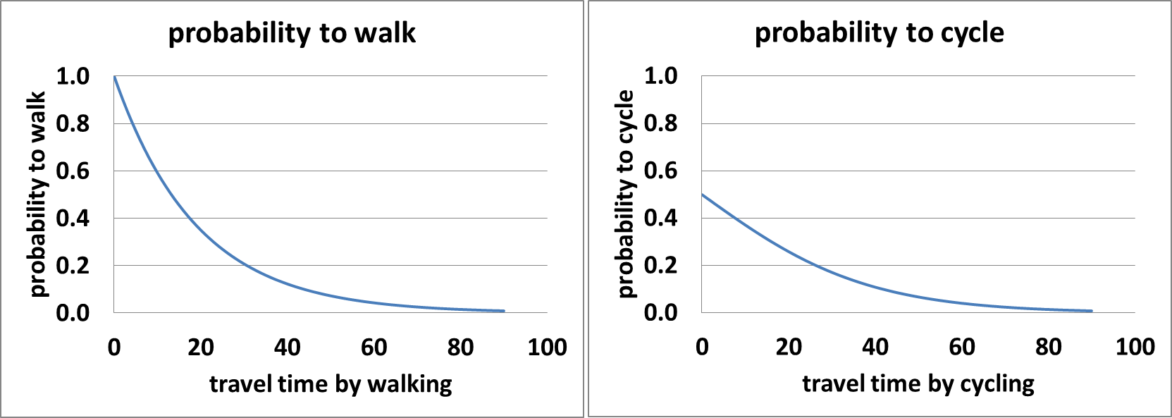
The formulas used for computing the probabilities of walking (P(walk)) and cycling (P(cycle)) are:
| $$P(walk)=\frac{1}{1.3^{\frac{t_{walk}}{5}}}$$ | (1) |
| $$P(cycle)=\frac{1}{1+1.3^{\frac{t_{cycle}}{5}}}$$ | (2) |
Drivers’ Route Choosing Behaviour
Before every commute, drivers recall the level of congestion they experienced on roads they have used, and based on that information choose the fastest routes using Dijkstra’s route-finding algorithm (Skiena 1990). If a driver has never driven on a road section before, she will assume no congestion and that she can drive at the speed limit on that road, until her experience proves otherwise. If a driver has driven on a road section before, and the level of congestion she experiences this time is different than in her memory, she updates her memory and uses the latest information for future route choice. We assume that drivers use travel time as the only criterion when choosing route. They do not consider other factors such as scenery and the number of traffic lights, which in reality can also affect route choice (Khattak et al. 1993; Zhang & Levinson 2008).
Cyclists also choose the fastest route to work using Dijkstra’s algorithm. The difference is that cyclists do not need to update route choice each day because their journey time is assumed not to be affected by congestion level, since they can always go in front of and between cars to move forward. Unlike cyclists and drivers who have to travel via principal road, we assume that walkers can travel via the most direct route that connects home and work, given that sidewalk networks usually have better coverage and connections than principal roads.
Driving Behaviour
This paper also adopts the car-following driving rule and the assumption of single lane traffic typical in TCA models discussed in Section 2. However, compared with a typical TCA model, space is modelled with a much coarser grain (100m) than the more usual 7.5m. Since we are simulating daily commuting behaviour in an area of roughly 2000 km2, modelling at finer resolutions would be impractical: 7.5m wide cells would require 36M patches as opposed to 200,000 patches at 100m.
We assume that a vehicle speeds up at the acceleration rate and drives at the speed limit on that road until there is car in the patch ahead of it. Then it slows down at the deceleration rate and follows the car ahead. We assume a single-lane in each direction, with no overtaking.
Whether cars will meet cyclists on the road depends on whether the parameter “cyclist sharing roads” is true. If true, cyclists and cars will have to share road space, and we assume that if a cyclist is in front of a car on the road, the car will have to stop and wait for the cyclist for one time step in the model (2.8s). After that, the car can overtake the cyclist. If false, then cyclists and cars do not share space on the road, as if there is a separate cycle lane. We assume that pedestrians are always separated from cars and cyclists.
CO2 Emissions Model
The CO2 emission model we use in the model is developed by Cappiello et al. (2002) for Category 9 vehicles in the United States. The authors estimated a statistical model of CO2 emissions for cars under Tier 1 emission standard (roughly equivalent to Euro 1). Tailpipe emissions are estimated as a function of speed ( v) and acceleration ( a). Since we are only interested in relative emissions values, using formulas calibrated on older vehicles is not anticipated to significantly affect the results. Equation 3 shows the estimated tailpipe CO2 emission as a function of speed and acceleration:
| $$ TP_{CO_2}= \begin{cases} 1.02+.0118v+1.92e-06v^3+.224av, & v>0 \\ .877, & v=0 \end{cases}$$ | (3) |
Equation 3 reflects that steady-speed driving is less polluting than driving with frequent acceleration and deceleration, which is confirmed by empirical evidence (Tong et al. 2000).
Treatment Factors and Experiment Design
There are four treatment factors in the model: flexitime range (f), urban concentration (u), bypass (b), and cyclist (sharing roads) (c). The first two treatments are continuous, whereas the last two are Boolean.
Flexitime is a time range within which employees can choose when to arrive at work. For example, employees may choose to arrive at work anytime between 7:30am to 9:30am and, depending on the time of arrival, leave work between 4pm to 6pm. The larger the range, the more flattened and spread-out the peak hour would be. Flexitime is measured in number of minutes.
Urban concentration measures the proportion of population living in the urban area. An urban area is defined as level 1 in Rural-Urban Classification in Figure 2. To simulate different levels of urbanization, we construct an urban concentration index by over-sampling population in urban or rural areas, depending on the index. For example, an urban concentration index of four means that agents are four times more likely to live in an urban area (most of the City of Aberdeen) than now. Likewise, an urban concentration index of 0.25 means that agents are 75% less likely to live in an urban area than now. Formally, for urban concentration index u, the re-sampled proportion of urban population, \(\widehat{p_u(x)}\):
| $$\widehat{p_u(u)}=\frac{p_u \cdot u}{p_u \cdot u+(1-p_u)}=1-\frac{1-p_u}{p_u \cdot u+(1-p_u)}$$ | (4) |
The third treatment, bypass, refers to the AWPR (featured as a yellow line in Figure 1 and 2). If b is false, the simulated road network represents the one we currently have; whereas if b is true, it represents the road network we will have after the completion of the new bypass in 2017.
The last treatment, cyclist (sharing roads with cars), refers to whether cyclists and cars share the same roads. If c is true, cars will have to stop and wait for the cyclists to pass, as discussed in Section 3.5.2. If c is false, cars and cyclists stay on separate paths and do not interfere with each other. We will test if cyclists indeed interfere and slow down the traffic, given the assumption in the model.
One of the contributions of this paper is that we not only examine the effect of each treatment factor with others held constant as most previous studies do, but also analyse the different connections of these factors in order to detect the cumulative effects of them. Therefore, instead of studying each factor in isolation and design single policy around it, we are able to look at the diverse conflation of the four treatment factors and help design integrated policy that covers different aspects such as social, urban and infrastructural.
Turning to the experimental design, a prior analysis (Ge & Polhill 2015) has shown that the results are more sensitive to changes in flexitime range when it is less than 60 minutes. Therefore we sample flexitime more densely between 0 and 60. We sample the urban concentration index so that it represents five scenarios where agents are 75% less likely, 50% less likely, as likely, two times more likely and four times more likely to live in an urban area than they are now.
Table 5 summarizes the treatment factors and experiment design for the simulation.
| Treatment Factor (symbol) | Parameter space | Experiment design |
|---|---|---|
| Flexitime range (f) | [0, ) minutes | (0, 15, 30, 60, 120) minutes |
| Urban concentration (u) | [0, ) | (0.25, 0.5, 1, 2, 4) |
| Bypass (b) | True, false | True, false |
| Cyclists and drivers share roads (c) | True, false | True, false |
Results and Discussion
CO2 Emissions
This section reports the effect of each of the treatment factors on CO2 emissions. We first show the effect of each of the four treatment factors on CO2 emissions in a typical morning peak, with all the other treatment factors fixed at their default values. Then we show the combined effect of all the treatment factors using a regression analysis.
Figure 4 shows the effect of flexitime on CO2 emissions, while fixing urban concentration at 1, bypass at false and cyclist at true. We find that CO2 emissions distribution in peak hours is more spread-out under longer flexitime range. As we will see later, longer flexitime also reduces total CO2 emissions.
Figure 5 shows the effect of urban concentration on CO2 emissions, while fixing flexitime at 30, bypass at false and cyclist at true: that higher urban concentration reduces CO2 emissions, because agents then live closer to work on average, leading to higher P(walk) and P(cycle).
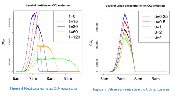
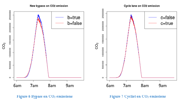
Figure 6 shows the effect of bypass on CO2 emissions, while fixing flexitime at 30, urban concentration at 1 and cyclist at true. We find that the new bypass will cause CO2 emissions to increase slightly, because it provides the commuters with a longer but faster route option. Finally, Figure 7 shows the effect of cyclists sharing roads with cars on CO2 emissions, while fixing flexitime at 30, urban concentration at 1 and bypass at false. We show that in general, car sharing roads with the cyclists does not alter total CO2 emissions from traffic.
Figures 4 through 7 show the effect of each treatment on CO2 emissions, with the other treatments fixed at their default levels. The combined effect of all the treatments is shown in the regression analysis in Table 6, which uses the logarithm of total CO2 emissions. Since for each parameter combination we ran the simulation for 10 times with a different random seed at each time, we used a two-level random effect model. Each parameter combination is treated as a group, and as a result there are 10 data points within each group. The results in Table 6 are consistent with those indicated in Figures 4 through 7.
| log(CO2) | Coef. | Std. Err. | P>z | [95% Conf. | Interval] |
|---|---|---|---|---|---|
| f = 0 | 0.002 | 0 | 0 | 0.001 | 0.002 |
| f = 15 | 0.002 | 0 | 0 | 0.001 | 0.002 |
| f = 30 (default) | |||||
| f = 60 | -0.001 | 0 | 0.042 | -0.001 | 0 |
| f = 120 | -0.002 | 0 | 0 | -0.002 | -0.001 |
| u = 0.25 | 0.039 | 0 | 0 | 0.039 | 0.04 |
| u = 0.5 | 0.02 | 0 | 0 | 0.019 | 0.021 |
| u = 1 (default) | |||||
| u = 2 | -0.016 | 0 | 0 | -0.017 | -0.015 |
| u = 4 | -0.027 | 0 | 0 | -0.028 | -0.026 |
| bypass=true (default=false) | 0.002 | 0 | 0 | 0.001 | 0.002 |
| cyclist=false (default=true) | 0 | 0 | 0.453 | -0.001 | 0 |
| intercept | 28.27 | 0 | 0 | 28.27 | 28.271 |
Table 6 shows that reducing flexitime from the default level of 30 minutes to 15 minutes will increase CO2 emissions by 0.2%, because of increased traffic congestion. Interestingly, there is no difference in CO2 emissions between 0 and 15 minutes flexitime, which suggests 15 minutes are insufficient to dissipate traffic. On the other hand, doubling flexitime from 30 to 60 minutes will reduce CO2 emissions by 0.1%, and further increasing flexitime from 60 to 120 minutes will reduce CO2 emissions by another 0.1%. We conclude that changing flexitime has a larger impact on CO2 emissions when existing flexitime is relatively low; in other words, the marginal benefit from flexitime decreases as flexitime increases.
Table 6 shows that reducing urban concentration will significantly increase CO2 emissions. The current level of urban concentration is, by definition, u = 1. If u > 1, residences are more concentrated geographically than at present; whereas they are less concentrated if u < 1. If u = 0.5, CO2 emissions from commuting will increase by 2%. Moreover, if u = 0.25, CO2 emissions from commuting will increase by 3.9%. On the other hand, if u = 2, CO2 emissions from commute will decrease by 1.6%, and if u = 4, CO2 emissions from commuting will decrease by 2.7%. People living in large urban areas are more likely to live closer to work, therefore they are more likely to choose walking or cycling as their transport mode. Even if they drive they will drive a shorter distance on average.
Previous findings are mixed regarding the relationship between urban concentration and CO2 emissions. For example, Glaeser and Kahn (2010) looked at U.S. cities and found that areas with high urban concentration are generally associated with lower carbon emissions compared with suburban areas; whereas Bo and Jianfeng (2014) examined Chinese cities and found that emissions per GDP unit first increases and then decreases with urban concentration. In this paper we only look at CO2 emissions from driving, and have not taken into account other emission sources such as property construction and home energy use. As a result, we cannot conclude on the relationship between general emission level from all sources and urban concentration. However, we do find that high urban concentration is associated with less emission from transport in the model. Moreover, even though the inner city has more traffic and possibly more emissions from higher urban concentration, overall the entire region benefits from more concentrated living. Therefore we argue that the impact of urban policies should never be examined in the urban areas alone. Its impact on surrounding areas should also be taken into account.
Regarding the impact of the AWPR, Table 6 shows that having the bypass will increase total CO2 emissions by 0.2%, probably because the bypass offers a faster but longer route. Finally, we find that cyclists sharing roads with drivers do not change CO2 emissions.
Commute Time
Mean Commute Time
This section reports the effects of treatment factors on mean commute time to work. Each simulation contains 60 days. The first 20 days are disregarded as a burn-out period; commute time in the last 40 days are collected for analysis. Each simulation contains 1000 commuting agents. Since we run the simulation 10 times for each parameter combination, we have daily commute times of 10,000 agents for 40 days from every parameter combination. The curves in Figures 8 through 11 show the kernel probability density of mean commute time over 40 days of 10,000 simulated agents. The vertical lines show the average mean commute time of all agents. For presentation purposes, travel time is curtailed at 60 minutes on the graph.
Figure 8 shows the probability density curves of mean commute time with different flexitimes, while fixing u = 1, b = false, and c = true. Increasing flexitime reduces daily commute time. Increasing flexitime from zero minutes to two hours will save on average 5 minutes in commute time to work, but with diminishing marginal returns as flexibility increases above 15 minutes.
Figure 9 shows the probability density curves of mean commute time with different levels of urban concentration, while fixing f = 30, b = false, and c = true. We find that higher urban concentration reduces mean commute time, mostly because people are more likely to live close to work if they live in large urban area. We find that the time saving is relatively small from doubling urban concentration from one to two or from two to four. We believe the main reason is that Aberdeen City and suburbs is relatively concentrated already, so the gain from becoming even more concentrated is relatively small, given the existing transport infrastructure. On the other hand, reducing the level of urban concentration will increase commute time more significantly.
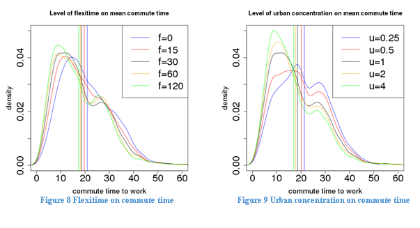
Figure 10 shows the effect of adding the AWPR bypass on the distribution of mean commute time. Adding the bypass will reduce commute time, but by a smaller amount than flexitime or urban concentration. Figure 11 shows the effect of cyclists sharing roads with drivers on the distribution of mean commute time, while fixing f = 30, u = 1, and b = false: cyclists do not increase mean commute time on the whole.

Figures 8 through 11 show the effects of each treatment on mean commute time distribution, with the other treatments fixed at their default levels. Table 7 shows the regression result of mean commute time on all the treatment factors. Again, we use a two-level random effect model to tackle multiple data points for each parameter combination. The results in Table 7 are consistent with those indicated in Figure 8 through Figure 11.
Table 7 shows that increasing flexitime allowed will reduce commute time. For example, increasing flexitime from 0 to 15 minutes will lead to a 7.3% reduction in mean commute time; and increasing flexitime from 15 to 30 minutes will lead to a 4.7% reduction in mean commute time. We therefore conclude that although increasing flexitime will always reduce commute time, the marginal benefit of flexitime diminishes as flexitime increases, which is consistent with the indication of Figure 9.
Table 7 shows that increasing urban concentration will reduce commute time. Specifically, if urban concentration goes from one to two, mean commute time will decrease by 5.3% on average. If people are four times as likely to live in Aberdeen City as they are now, mean commute time will decrease by 9.2% on average. On the other hand, if urban concentration goes from one to a half, mean commute time will increase by 6.9% on average, and from one to a quarter, mean commute time will increase by 13.9% on average.
Congestion and pollution in large urban areas are generally regarded as “city problems”, and measures like green belts have been taken to limit the expansion of cities. It is also observed that as people become wealthier they tend to move away from city centre for more living space in the suburbs. On the other hand, there have been trends of restoration and reinvention of city centres (gentrification) in large cities like London and Washington D.C. (Lees et al. 2013). De-urbanization and gentrification are much broader social issues beyond commuting. Yet our model suggests that although higher urban concentration may cause more congestion and pollution in urban areas, overall it reduces mean commute time and CO2 emissions from traffic. The result indicates that urban issues should not be studied in isolation from its surroundings. In an attempt to tackle issues in urban areas, policymakers should make sure that problems are not exported to the surrounding areas.
Table 7 shows that the bypass will reduce mean commute time by 2.1%. Finally, it shows that having cyclists share roads with cars will not increase mean commute time, while controlling for the other three treatments.
| log (mean commute time) | Coef. | Std. Err. | P>z | [95% Conf. | Interval] |
|---|---|---|---|---|---|
| f = 0 | 0.12 | 0.003 | 0 | 0.115 | 0.125 |
| f = 15 | 0.047 | 0.003 | 0 | 0.042 | 0.052 |
| f = 30 (default) | |||||
| f = 60 | -0.035 | 0.003 | 0 | -0.04 | -0.03 |
| f = 120 | -0.06 | 0.003 | 0 | -0.065 | -0.055 |
| u = 0.25 | 0.139 | 0.003 | 0 | 0.134 | 0.144 |
| u = 0.5 | 0.069 | 0.003 | 0 | 0.064 | 0.074 |
| u = 1 (default) | |||||
| u = 2 | -0.053 | 0.003 | 0 | -0.058 | -0.048 |
| u = 4 | -0.092 | 0.003 | 0 | -0.097 | -0.087 |
| bypass=true (default=false) | -0.021 | 0.002 | 0 | -0.024 | -0.018 |
| cyclist=false (default=true) | 0 | 0.002 | 0.843 | -0.003 | 0.003 |
| intercept | 2.923 | 0.003 | 0 | 2.918 | 2.928 |
Commute Time Reliability
This section examines the effect of treatment factors on commute time reliability. In addition to commute time, commute time reliability is another key factor in travellers’ decision-making. A large variance in travel time is considered as an important added cost to travellers (Jackson & Jucker 1982), because travellers need to allow “buffer time”, and the more unreliable travel time is, the more buffer time is needed. We use standard deviation of commute time over mean commute time for each individual over 40 days as the indicator for commute time reliability. The larger the standard deviation over mean commute time, the more unreliable commute time is.
Figure 12 shows the kernel probability density function of standard deviation over mean commute time with different levels of flexitime allowances. Reducing flexitime allowance below 30 minutes or eliminating it altogether does not only increase commute time, as is shown previously, it also significantly increases the unreliability of commute time, probably due to more time spent in traffic jams. This indicates that there is a double dividend from introducing flexitime arrangement: allowing some flexitime will not only dissipate peak emissions and reduce mean commute time, it will also make travel time more predictable.
Moreover, a flexitime arrangement can add a third time-saving benefit if it further reduces buffer time by loosening the requirement to be “on time” all the time. For example, with no flexitime allowance, an employee may have to ensure that she arrives at work before the starting time for most of the time, say, 95% of the time, to keep her probability of being late for work below 5%. Under flexible working time arrangements, an employee can cut down on that probability. She may only aim at arriving at work by a certain time for half of the time instead of 95%, provided the target time to arrive at work is a suitable period before the latest time the flexible working arrangements allow. This added flexibility allows employees to further cut down on their buffer time now that they are less worried about being “on time” all the time.
To illustrate this, we calculate the 95% percentile commute time under zero flexitime and 50% percentile commute time under 30-minute flexitime for each individual. Figure 13 shows the differences in commute time when buffer time is taken into account. It is clear that when travel time unreliability and buffer time is taken into account, the potential time saving from flexitime arrangements could be more substantial.
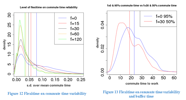
Table 8 shows the regression results of log of travel time variability. We find that reducing flexitime from 30 to 0 will increase travel time variability by 55.1%, and reducing flexitime from 30 to 15 minutes will increase travel time variability by 20.3%. On the other hand, increasing flexitime will reduce travel time variability: increasing flexitime from 30 to 60 minutes will reduce travel time variability by 21%, and increasing flexitime from 30 to 120 minutes will reduce travel time variability by 33.6%.
Regarding urban concentration, we find that higher urban concentration increases travel time variability. The regression results show that if people are twice as likely to live in Aberdeen City (u = 2), travel time variability will be increase by 6.1%, and if people are four times more likely to live in urban areas (u = 4), travel time variability will increase by 10.2%. On the other hand, if people are half as likely to live in Aberdeen City (u goes from one to 0.5), travel time variability will decrease by 8.2%, and if u goes from one to 0.25, travel time variability will decrease by 15.9%.
Interestingly, we learn from Section 5.2.1 that mean commute time is lower when urban concentration is high. In this section, however, we show that commute time variance increases as urban concentration goes up, which does not necessarily contradict the findings in 5.2.1, but indicates a trade-off exists between commute time length and reliability for those choosing to drive. High urban concentration will lead to low travel time as people in the city are on average closer to work. On the other hand, high urban concentration will also cause more variability in travel time, as the city becomes more congested. The time savings achieved by commuters moving closer to the city may be partially offset by longer buffer time needed by commuters as travel time becomes less reliable. Therefore, when designing urban or transport policies, policymakers should not only consider the travel time length, but also travel time reliability, knowing that there might be a trade-off between the two. Finally, we find that neither bypass nor cyclist treatments has altered travel time reliability.
| log (sd/mean) | Coef. | Std. Err. | P>z | [95% Conf. | Interval] |
|---|---|---|---|---|---|
| f = 0 | 0.551 | 0.012 | 0 | 0.528 | 0.575 |
| f = 15 | 0.203 | 0.012 | 0 | 0.18 | 0.226 |
| f = 30 (default) | |||||
| f = 60 | -0.21 | 0.012 | 0 | -0.234 | -0.187 |
| f = 120 | -0.336 | 0.012 | 0 | -0.359 | -0.313 |
| u = 0.25 | -0.159 | 0.012 | 0 | -0.182 | -0.136 |
| u = 0.5 | -0.082 | 0.012 | 0 | -0.105 | -0.059 |
| u = 1 (default) | |||||
| u = 2 | 0.061 | 0.012 | 0 | 0.038 | 0.084 |
| u = 4 | 0.102 | 0.012 | 0 | 0.079 | 0.125 |
| bypass=true (default=false) | -0.009 | 0.008 | 0.213 | -0.024 | 0.005 |
| cyclist=false (default=true) | -0.004 | 0.008 | 0.576 | -0.019 | 0.011 |
| Intercept | -3.102 | 0.012 | 0 | -3.126 | -3.078 |
Model Validation
We use the Transport Model for Scotland 2012 (TMFS12) (Lumsden et al. 2007; Transport Scotland 2015c, 2015d) to validate our simulation results. TMFS12 is developed and maintained under Transport Scotland’s Land Use and Transport Integration in Scotland service (LATIS) (Transport Scotland 2015b). The model is based on the four-stage transport demand model that includes trip generation, mode choice, destination choice and route choice. It extends the conventional four-stage model by including trip frequency choice, park and ride station choice and choice of high occupancy vehicle. Each stage of the model is calibrated using empirical data, including census travel-to-work data, Scottish Household Survey data, travel survey data and planning data (Transport Scotland 2015d).
The model divides the area into 38 zones of roughly equal population. Since areas near Aberdeen City are more densely populated, zones there are smaller. TMFS12 derives travel time for cars commuting to workplaces during morning peak hours between every pair of zones, with which we will compare our travel time estimates. Since the TMFS12 model projects commute time in both 2012 and 2019 (after AWPR is completed), we will compare our model results with the TMFS12 estimates both before and after AWPR. We assume that the default flexitime range is 30 minutes, with u = 1 and c = true. All other model parameters are the same as the ones we use to generate model results (Table 4).
Table 9 compares the estimated mean travel time from TMSF12 and this model. We find that in both cases our estimated mean travel time is less than that from TMSF12. The percentage reduction in travel time by AWPR is estimated to be 3.3% from our model simulation and 7% from TMSF12. Table 10 shows the mean absolute percentage difference in travel time between our model and TMSF12. On average, the mean simulated travel time from our model deviates from that from TMSF12 by a little less than 20%. Moreover, in the majority of the cases, our model produces a smaller travel time than TMSF12.
| Mean travel time between zones before AWPR (in minutes) | Mean travel time between zones after AWPR (in minutes) | Estimated % reduction in travel time by AWPR | |
|---|---|---|---|
| TMSF12 | 21.8 | 20.2 | 7% |
| This model | 18.3 | 17.7 | 3.3% |
| Mean abs. % difference in travel time between this model and TMSF12 | Prob. travel time from this model smaller than that from TMSF12 | |
|---|---|---|
| Before AWPR | 19.3% | 79.7% |
| After AWPR | 18.9% | 69.7% |
There are several reasons why the simulated travel time from our model can be different from the ones predicted by TMSF12. First, our model represents a simplified version of the traffic and does not include traffic controls such as traffic lights and stop signs. This partially explains why our simulated travel time is generally smaller than the one estimated by TMSF12. Second, our model only simulates commuting traffic, not other traffic that may interfere with the commute, such as the ‘school run’, deliveries (particularly lorries and vans, which have lower speed limits on rural roads), and other business-to-business interaction. Third, as shown in Figures 14 and 15, for some zones such as Banchory and Torphins, our model only includes the eastern part of them, not the entire zones. As a result, the simulated travel time to and from those zones is expected to be smaller than is predicted by TMSF12, which includes the entire zones. Finally, since travel time is only calculated between zones, travel time within zones is zero by definition in TMSF12. By contrast, travel time within zones is non-zero in our model.
Figure 14 and 15 shows the mean absolute percentage difference in travel time between our model and TMSF12 from and to the zones respectively. We notice that estimated travel time to and from Torphins has larger deviation from the TMSF12 estimation, probably due to exclusion of the western part of the zone in our model, though similar exclusions occur in other zones. We also find that estimated travel time to and from zones that are smaller and more densely populated has smaller deviation from the TMSF12 estimation on average. This may be caused by two reasons. First, because traffic is less congested in less densely populated zones, cars are more likely to drive at the speed limit without interference in those areas in our model. As a result, the impacts of not having traffic lights and stop signs could be more significant. Second, since home and work location is randomly assigned using address data (see Section 3.4), and there are fewer homes and businesses in the less populated zones, any misspecification in home and work location will have a larger impact in travel time in those zones.


With reference to Axtell et al. (1996)’s standards of model replication, we have achieved ‘relational alignment’ of our agent-based model with TMFS12, in that the two models show the same direction of effect of the bypass. We therefore believe that our simulation has captured the fundamental dynamics of daily commute in the area, and our estimated travel time is in line with the travel time predicted by TMFS12 both before and after AWPR. Although the model tends to produce lower travel time estimates than TMFS12, partially due to the reasons mentioned above, the system dynamics simulated in the model and the comparative analysis results should hold.
Conclusion
This paper describes an agent-based model of the daily commute in Aberdeen City and Shire. We have conducted a case study of Aberdeen area and explored various factors that affect daily commute patterns and their environmental consequences. Specifically, we examine the impact of flexitime arrangements, urban concentration, the new bypass and cycle lane on CO2 emissions, mean travel time and travel time reliability. We analyse the diverse conflation of the four treatment factors, explore different connections between them, and examine their aggregate effects.
We find that having a moderate amount of flexitime such as 30 minutes can significantly reduce CO2 emissions and flatten the peak of CO2 emissions during rush hours. However, the effectiveness of flexitime in reducing total CO2 emissions declines as more flexitime is allowed. Flexitime also reduces mean travel time and travel time variability. Again, the effect is more significant in comparison with no or little flexitime being allowed. Moreover, it provides additional time-saving benefits if it eliminates employees’ need to be on time all the time. We find that higher urban concentration leads to lower CO2 emissions from transport, but it also increases travel time variability. Regarding the impact of the new bypass, our model suggests that it does decrease mean commute time, but not by much. It also slightly increases CO2 emissions from traffic. Finally, we show that cyclists do not necessarily slow down traffic on the whole when sharing the road with cars.
In developing the model, we have made several simplifying assumptions due to space and scope limitation, and as a result the model can be extended in various ways. For example, it could include other driving activities, such as the ‘school run’ and shopping trips, or business-to-business traffic throughout the working day. It could consider the characteristics of the roads, such as slope, especially in walking and cycling. It could look at the impact of different driving styles and vehicle capabilities (particularly acceleration). It could investigate the impact of other variables, such as urban structure, green areas and dominant winds on CO2 concentration and commute behaviour. Other features such as traffic controls and public transport could also be added.
Acknowledgements
This work was funded by the European Commission under Framework Programme 7, grant agreement number 613420 (GLAMURS).References
ABDEL-ATY, M. A., & Abdalla, M. F. (2006). Examination of multiple mode/route-choice paradigms under ATIS. Intelligent Transportation Systems, IEEE Transactions, 7(3), 332-348. [doi:10.1109/TITS.2006.880634]
ABERDEEN CITY COUNCIL (2015). Aberdeen Stats and Facts. from http://liv.ac.uk.libanswers.com/a.php?qid=349952
ADLER, J. L. (2001). Investigating the learning effects of route guidance and traffic advisories on route choice behavior. Transportation Research Part C: Emerging Technologies, 9(1), 1-14. [doi:10.1016/S0968-090X(00)00002-4]
ARSLAN, T., & Khisty, J. (2006). A rational approach to handling fuzzy perceptions in route choice. European Journal of Operational Research, 168(2), 571-583.
ASENSIO, J., & Matas, A. (2008). Commuters’ valuation of travel time variability. Transportation Research Part E: Logistics and Transportation Review, 44(6), 1074-1085. [doi:10.1016/j.tre.2007.12.002]
AVINERI, E., & Prashker, J. N. (2005). Sensitivity to travel time variability: Travelers’ learning perspective. Transportation Research Part C: Emerging Technologies, 13(2), 157-183.
AXTELL, R., Axelrod, R., Epstein, J. M., & Cohen, M. D. (1996). Aligning simulation models: A case study and results. Computational & Mathematical Organization Theory, 1(2), 123-141. [doi:10.1007/BF01299065]
BARTH, M., & Boriboonsomsin, K. (2008). Real-world carbon dioxide impacts of traffic congestion. Transportation Research Record: Journal of the Transportation Research Board (2058), 163-171.
BATLEY, R., & Ibáñez, J. N. (2012). Randomness in preference orderings, outcomes and attribute tastes: An application to journey time risk. Journal of Choice Modelling, 5(3), 157-175. [doi:10.1016/j.jocm.2013.03.003]
BENJAMIN, S. C., Johnson, N. F., & Hui, P. (1996). Cellular automata models of traffic flow along a highway containing a junction. Journal of Physics A: Mathematical and General, 29(12), 3119.
BHAT, C. R., & Sardesai, R. (2006). The impact of stop-making and travel time reliability on commute mode choice. Transportation Research Part B: Methodological, 40(9), 709-730. [doi:10.1016/j.trb.2005.09.008]
BO, Q., & Jianfeng, W. (2014). Does urban concentration mitigate CO 2 emissions? Evidence from China 1998–2008. China Economic Review.
CAPPIELLO, A., Chabini, I., Nam, E. K., Lue, A., & Abou Zeid, M. (2002). A statistical model of vehicle emissions and fuel consumption. Paper presented at the Intelligent Transportation Systems, 2002. Proceedings. The IEEE 5th International Conference on. [doi:10.1109/itsc.2002.1041322]
CIOFFI-REVILLA, C., & Gotts, N. (2003). Comparative analysis of agent-based social simulations: GeoSim and FEARLUS models. Journal of Artificial Societies and Social Simulation, 6(4) 10: https://www.jasss.org/6/4/10.html.
DEPARTMENT FOR TRANSPORT (2012). Guidance on Road Classification and the Primary Route Network. from https://www.gov.uk/government/uploads/system/uploads/attachment_data/file/315783/road-classification-guidance.pdf
DIA, H. (2002). An agent-based approach to modelling driver route choice behaviour under the influence of real-time information. Transportation Research Part C: Emerging Technologies, 10(5–6), 331-349.
DUIJN, M., IMMERS, L., Waaldijk, F., & Stoelhorst, H. (2003). Gaming Approach Route 26: a combination of computer simulation, design tools and social interaction. Journal of Artificial Societies and Social Simulation, 6(3) 7: https://www.jasss.org/6/3/7.html.
EUROPEAN COMMISSION (2016). Road transport: Reducing CO2 emissions from vehicles.
FIGLIOZZI, M. A. (2011). The impacts of congestion on time-definitive urban freight distribution networks CO2 emission levels: Results from a case study in Portland, Oregon. Transportation Research Part C: Emerging Technologies, 19(5), 766-778. [doi:10.1016/j.trc.2010.11.002]
GARGIULO, F., Lenormand, M., Huet, S., & Espinosa, O. B. (2012). Commuting network models: Getting the essentials. Journal of Artificial Societies and Social Simulation, 15(2), 6: https://www.jasss.org/15/2/6.html.
GAVER JR, D. P. (1968). Headstart strategies for combating congestion. Transportation Science, 2(2), 172-181. [doi:10.1287/trsc.2.2.172]
GE, J., & Polhill, G. (2015). Preliminary results from an agent-based model of the daily commute in Aberdeen and Aberdeenshire, UK Proceedings of The Eleventh Conference of the European Social Simulation Association.
GLAESER, E. L., & Kahn, M. E. (2010). The greenness of cities: Carbon dioxide emissions and urban development. Journal of Urban Economics, 67(3), 404-418. [doi:10.1016/j.jue.2009.11.006]
GOV.UK (2015a). Speed Limits. from https://www.gov.uk/speed-limits
GOV.UK (2015b). Typical stopping distances. from https://www.gov.uk/government/uploads/system/uploads/attachment_data/file/312249/the-highway-code-typical-stopping-distances.pdf
GOV.UK (2016). Transport emissions. from https://www.gov.uk/government/policies/transport-emissions
GRIMM, V., Berger, U., Bastiansen, F., Eliassen, S., Ginot, V., Giske, J., Goss-Custard, J., Grand, T., Heinz, S. K., & Huse, G. (2006). A standard protocol for describing individual-based and agent-based models. Ecological Modelling, 198(1), 115-126. [doi:10.1016/j.ecolmodel.2006.04.023]
GRIMM, V., Berger, U., Deangelis, D. L., Polhill, J. G., Giske, J., & Railsback, S. F. (2010). The ODD protocol: a review and first update. Ecological Modelling, 221(23), 2760-2768.
JACKSON, W. B., & Jucker, J. V. (1982). An empirical study of travel time variability and travel choice behavior. Transportation Science, 16(4), 460-475. [doi:10.1287/trsc.16.4.460]
KHATTAK, A. J., Koppelman, F. S., & Schofer, J. L. (1993). Stated preferences for investigating commuters' diversion propensity. Transportation, 20(2), 107-127.
KLÜGL, F., & Bazzan, A. L. (2004). Route decision behaviour in a commuting scenario: Simple heuristics adaptation and effect of traffic forecast. Journal of Artificial Societies and Social Simulation, 7(1) 1: https://www.jasss.org/7/1/1.html.
KNIGHT, T. E. (1974). An approach to the evaluation of changes in travel unreliability: a “safety margin” hypothesis. Transportation, 3(4), 393-408.
LÁRRAGA, M., DEL Río, J., & MEHTA, A. (2002). Two effective temperatures in traffic flow models: analogies with granular flow. Physica A: Statistical Mechanics and its Applications, 307(3), 527-547. [doi:10.1016/S0378-4371(01)00583-0]
LÁRRAGA, M. E., Río, J. A. D., & Alvarez-Lcaza, L. (2005). Cellular automata for one-lane traffic flow modeling. Transportation Research Part C: Emerging Technologies, 13(1), 63-74.
LEES, L., Slater, T., & Wyly, E. (2013). Gentrification. Routledge.
LUMSDEN, K., Gillies, H., & Canning, S. (2007). Transport Model for Scotland–A National Treasure. Paper presented at the 11th World Conference on Transport Research.
MA, T., Zhao, J., Xiang, S., Zhu, Y., & Liu, P. (2014). An Agent-Based Training System for Optimizing the Layout of AFVs' Initial Filling Stations. Journal of Artificial Societies and Social Simulation, 17(4) 6: https://www.jasss.org/17/4/6.html. [doi:10.18564/jasss.2570]
MAERIVOET, S., & De Moor, B. (2005). Cellular automata models of road traffic. Physics Reports, 419(1), 1-64.
MAHMASSANI, H. S., & Liu, Y. H. (1999). Dynamics of commuting decision behaviour under advanced traveller information systems. Transportation Research Part C: Emerging Technologies, 7(2), 91-107. [doi:10.1016/S0968-090X(99)00014-5]
MALIK, A., Crooks, A., Root, H., & Swartz, M. (2015). Exploring Creativity and Urban Development with Agent-Based Modeling. Journal of Artificial Societies and Social Simulation, 18(2), 12: https://www.jasss.org/18/2/12.html.
NAGATANI, T. (1993). Self-organization and phase transition in traffic-flow model of a two-lane roadway. Journal of Physics A: Mathematical and General, 26(17), L781. [doi:10.1088/0305-4470/26/17/005]
NAKAYAMA, S., Kitamura, R., & Fujii, S. (2001). Drivers' route choice rules and network behavior: Do drivers become rational and homogeneous through learning? Transportation Research Record: Journal of the Transportation Research Board, 1752(1), 62-68.
ONS (2011). Where do we commute to? Commuting patterns in the United Kingdom, 2011 Census. from http://www.neighbourhood.statistics.gov.uk/
ORDNANCE SURVEY (2015). Ordnance Survey Data. from https://www.ordnancesurvey.co.uk/
RAMMING, M. S. (2001). Network knowledge and route choice. Massachusetts Institute of Technology.
SIMON, P., & Nagel, K. (1998). Simplified cellular automaton model for city traffic. Physical Review E, 58(2), 1286.
SKIENA, S. (1990). Dijkstra's Algorithm. Implementing Discrete Mathematics: Combinatorics and Graph Theory with Mathematica, Reading, MA: Addison-Wesley, 225-227.
SPANGENBERG, J. H., & Lorek, S. (2002). Environmentally sustainable household consumption: from aggregate environmental pressures to priority fields of action. Ecological Economics, 43(2), 127-140.
STRAZDINS, L., & Loughrey, B. (2008). Too busy: why time is a health and environmental problem. New South Wales public health bulletin, 18(12), 219-221. [doi:10.1071/NB07029]
THE SCOTTISH GOVERNMENT. (2014). Scottish Government Urban Rural Classification. from http://www.gov.scot/Topics/Statistics/About/Methodology/UrbanRuralClassification
TISUE, S., & Wilensky, U. (2004). Netlogo: A simple environment for modeling complexity. Paper presented at the International conference on complex systems.
TONG, H., HUNG, W., & Cheung, C. (2000). On-road motor vehicle emissions and fuel consumption in urban driving conditions. Journal of the Air & Waste Management Association, 50(4), 543-554.
TRANSPORT SCOTLAND (2015a). Aberdeen Western Peripheral Route / Balmedie to Tipperty. from http://www.transportscotland.gov.uk/project/aberdeen-western-peripheral-route-balmedie-tipperty
TRANSPORT SCOTLAND (2015b). LATIS (Land Use and Transport Integration in Scotland). from http://www.transportscotland.gov.uk/LATIS
TRANSPORT SCOTLAND (2015c). National Transport and Land Use Models. Transport Model for Scotland (TMfS). 2015, from http://www.transportscotland.gov.uk/latis/national-transport-and-land-use-models
TRANSPORT SCOTLAND (2015d). TMFS12 Demand Model Development Report: Transport Scotland.
TRANTER, P. J. (2010). Speed kills: the complex links between transport, lack of time and urban health. Journal of Urban Health, 87(2), 155-166. [doi:10.1007/s11524-009-9433-9]
WANG, L., Wang, B.H., & Hu, B. (2001). Cellular automaton traffic flow model between the Fukui-Ishibashi and Nagel-Schreckenberg models. Physical Review E, 63(5), 056117.
WARDROP, J. G. (1952). Road Paper. Some Theoretical Aspects of Road Traffic Research. Paper presented at the ICE Proceedings: Engineering Divisions.
ZHANG, L., & Levinson, D. (2008). Determinants of route choice and value of traveler information: a field experiment. Transportation Research Record: Journal of the Transportation Research Board, 2086(1), 81-92.