
Introduction
In this paper, we present research where analytical results obtained in a simplified model are used to enhance our understanding of an already existing social simulation model. This shows that two techniques, agent-based modeling and probabilistic analysis, can be used jointly in some settings to provide further insights about a conceptual model. Here the original model was built to attain a theoretical understanding of abstract stylized facts. In the present paper, we will explain the differences between the modeling approaches, and how the second model, although much simpler, draws attention to the role of an important parameter we had not tested in the first version of the simulation model. We believe that this comparison between models can be of interest to the model-to-model research community. Indeed, we show that an analytical model can explain some properties of a simulation model and that it can also identify properties of the model that have an important impact on the results.
The first simulation model (we will refer to it as 'RT2012') enabled us to show that the presence of over-confident agents in a population can slow down collective learning (Rouchier & Tanimura 2012). The application we had in mind concerned the coordination of agents using a resource collectively. We consider a context where the diffusion of knowledge is important to reduce inefficiency and where knowledge diffusion depends on the success of the agents, which in turn depends on the quality of their belief. A correct belief is close to the reality of the environment and an incorrect belief is wrong in many dimensions. In the analytical model ('AM') we represent the accuracy of the beliefs in a much simpler way. Thus it is not necessarily the case that all the results obtained in this setting carry over to the simulation model.
In this new paper, we present RT2012 briefly but readers should refer to Rouchier & Tanimura (2012) for details. We then develop the analytical model which is shown to capture the main features of the original model but, as mentioned above, in a greatly simplified belief environment; proof of AM is placed in an appendix, but intuitions are developed in the main text. These results provide intuitions about the mechanism of RT2012, but also draws attention to some important features that would not have been tested in the simulations otherwise. As a short variation, we show that the analytical model can itself be simulated, in finite time and with finite population sizes, and that the time required for convergence is not too great. Combined, these two approaches allow us to identify a number of problems that arise in our dynamics of collective learning. We can then draw conclusions about the interest of using different modeling approaches to obtain a deeper knowledge of the processes at stake - which is one of the main claims of the M2M (model-to-model) research trend.
M2M
Since the beginning of the century, the M2M approach, as developed in two special issues in JASSS, has focused on the relation among models and the possibility of creating interactions between them (Hales et al.2003; Rouchier et al. 2008). This approach is all the more important since computerized simulation models can be subject to numerous errors, in the coding phase as well as in the simulation itself which relies on machine approximations (Polhill et al.2005). This can translate into wrong interpretations of the results in regard to the dynamics of the target system. Several techniques have been used to enhance the robustness and level of generality of computer models.
To assess the quality of the simulation results, whether they are already published or not, replication is the most widespread technique (although it is still possible to consider that it is not used enough (Wilensky & Rand 2007)). Replication enables us to criticize the imperfect quality of description of the model or results in a paper (Rouchier 2003), whose incompleteness makes it impossible to reproduce the dynamics of the formally described model. It can also, in a more fundamental way, show that some exposed results just do not hold, like in Edmonds and Hales (2003). They have also been used to extend model validity by focusing on parameters different from those in the original papers, as one has frequently done in the case of opinion dynamics (i.e. Urbig, Lorenz & Herzberg 2008). Failed replication and the response by the original modeler can also give rise to interesting and fundamental methodological discussions, like the "Deffuant discussion" (Meadows and Cliff 2012; Deffuant et al. 2013) (which reminds us that a simulator has to be aware of the importance of time to be able to draw conclusions), or the "Macy discussion" (Will & Hegselmann 2008; Macy & Sato 2008; Will 2009) (which reminds us all that devil is in the details).
A more difficult research agenda is the one that proposes to identify classes of models which display similar dynamics (Cioffi & Gotts 2003). This fundamental approach has the ambition to slowly build a theory of complex dynamics through the identification of common processes among seemingly different models that have common characteristics, although, at first sight, their fields of application are very different. To sustain this research trend (and also to solve the problem of incomplete description of models), a description protocol, the ODD protocol has been proposed and has since gained recognition and been widely used in various applications (Polhill et al. 2008). This protocol also enables us to compare structurally different models that deal with the same type of target system but with different modeling choices (Polhill et al. 2007). In general, exact explicitness, transparency and the open access to simulation models have been considered the most important basis for sharing scientific knowledge produced by simulation (see https://www.openabm.com and (Janssen et al. 2008).
Sometimes, research on the validation of generally identifiable social dynamics has also relied on the link between agent-based models and what can be described under the generic term of analytical models. The idea is to show that results that are observed through simulations can be proven to hold in a given set of situations, often described in more abstract terms (like in our case, which will be described later, with a population of agents whose size goes to infinity and who interact over a number of periods that also goes to infinity). As seen in the previously cited discussion about the Deffuant model, the convergence time can be extremely long, and the risk is to stop a simulation too early, believing that a steady state has been reached, whereas a new state could be attained if time was, for example, doubled. Maybe one answer to this very general problem could be provided by Grazzini (2012) who discusses, for cases where it is impossible to explicitly write the equations that regulate the evolution of the system, how tools from non parametric statistics can be used to detect whether time series generated by agent based models are stationary and stem from an ergodic process.
The issue of connections between models has been apprehended in different ways. The most straightforward approach is to compare different existing models and to look at the similarity of their results, like (Klüver & Stoica 2003) studying behaviors in a network and showing that results are similar. In the same spirit, Edwards et al. (2003) demonstrate that an aggregate and a distributed model of opinion diffusion converge only when there is just one attractor but diverge if there are two. Some authors decided to go from an already established simple model which can be treated analytically, and to relax the hypotheses to check if the results remain similar. This is the type of result obtained by Vila (2008), who starts out with a deterministic Bertrand competition model, and then adds assumptions about agents' behavior using a genetic algorithm - in the end, he obtains similar results with both tools, showing that loyalty should emerge in this competitive setting. An integration of statistical and agent-based models is achieved by Silverman (Silverman et al. 2013), who thus succeeds in producing predictions and explanations of demographic phenomena in parallel.
It is also possible to make the link between ABM and analytical work by first running simulations and then creating from the model a simplified generalization, as in Cecconi et al. (2010) who show that for the congestion model they study, it would not have been possible to construct an analytical model without having previously studied simulation dynamics. The complementarity of these approaches is such that insights from the simulations are crucial for developing the analytical model which in turn extends certain aspects of the simulated model. Moreover, the simulations capture fluctuations over time whereas the analytical model focuses on average quantities. This paper is the one that is the closest to the research we present here, especially in the way the modeling phases are articulated.
The simulation model
The model that has already been published, RT2012 (Rouchier & Tanimura 2012), (as an evolution of a previous model and analysis (Rouchier & Shiina 2007)) shows that, in a particular setting, overconfident agents can prevent a whole population from learning when learning is social, in the sense that it includes influence among agents. The model is based on simulations that take place in a universe whose "objective reality", as well as the representation that agents have of this environment, take the shape of a culture vector as in Axelrod's work (1997). The properties of our environment, as well as the agents' beliefs, are hence a string of 10 bits taking 0 or 1 as value. Agents are boundedly rational: they have to act on this environment, and this action is also the only way for them to acquire information about its characteristics: when they succeed in their action, they can infer that their representation is correct, and when they fail they know they have some incorrect beliefs. The accuracy of individual beliefs is defined as the fraction of "correct bits"; the accuracy of the collective belief is defined as the average accuracy. The actions undertaken by the Agents do not have any impact on the characteristics of the environment which stay unchanged in the time-scale of the simulation.
We also add an influence mechanism to this simple feed-back learning, namely that agents have to act by pair, and thus choose who will "lead the action" and define the right representation used to choose the action. Since we want to test the influence of heterogeneity of self-confidence, we build our agents accordingly; heterogenous in this dimension, as well as in their representation of the environment (randomly drawn at initialization).
The way a time-step takes place is such that:
- randomly paired, agents first decide which belief to use for organizing their action: the agents with highest confidence is the one who leads the action and uses his belief
- according to the accuracy of the belief (its adequacy to real characteristics), the agents are more or less successful in their action: note that we do not actually model the action, but a probability of success - the probability of success is linear with respect to the accuracy of the belief of the leading agent.
- when an action is successful, the agent who led the action influences the other one by transforming his belief (only one bit is transformed at a time).
The main result of our study is that the presence of some very confident agents, who on average overestimate their knowledge and cannot be influenced by others, slows down, and can even completely stop, the learning of the society as a whole. One can identify thresholds in the number of overconfident agents, that produce different patterns in the simulations. In particular, results depend on the probability of meetings between agents that can influence each other.
Two criticisms can be directed at this first model. First, it is rather complex: the "Axelrod-type setting" gives rise to dynamics that are hard to anticipate, as he notes himself. Perhaps due to its complexity, this type of opinion model has not produced as vast a literature, as, for example, the Deffuant influence model has. Hence, the validity of our results cannot be checked in coherence with a large number of related dynamics that could have been documented otherwise.
We thus had to check if our result was robust, and to understand some of the underlying mechanisms behind it. We decided to study an analytical model that would share the main features of our model, and test the stability asymptotically with respect to time and population size. The three features - that learning takes place through influence, that accurate knowledge increases the ability to influence, and that communication can be restricted - have hence been included in a much simpler model for which it is possible to identify steady states of the system and characterize the conditions under which they occur.
A Simplified Model of Belief Evolution
Defining the model
In this section, we study analytically a simplified version of belief evolution in the presence of confident agents. Admittedly some of the richness and complexity of the initial model is lost due to the simplifications. However studying the simplified model should allow us to shed some light on the mechanisms that operate in the previous one. To make the model tractable, we retain only the most basic features of our situation: there are several possible beliefs which are more or less correct. Beliefs that are more correct increase the probability of successful actions and thus of convincing one's peers. Agents' confidence in their own beliefs prevent them from engaging in joint actions with others whose beliefs are too different.
The main simplification will concern the belief environment. Beliefs about the environment take values \(b\in \{0,1,...,K\}\). We will assume that the true state of the world is K, which means that the difference K-b measures the degree of error in the agents belief compared to the true state of the world. An agent whose belief is K knows the true state of the world, an agent whose belief is 0 is maximally mistaken about the true state of the world. This belief space is one dimensional, as opposed to the multi-dimensional one in the general model. The belief environment presented here is not a special case of that in Rouchier and Tanimura (2012). The difference is not just a quantitative reduction in complexity but a qualitative difference. Now agents whose level of error is the same necessarily hold the same beliefs which was not necessarily the case in the more complex belief environment, agents could be "equally wrong" if they had the same number of incorrect bits, but not necessarily mistaken in the same way if their errors concerned different bits.
Let us now define what is meant by the confidence of an agent in this setting. An agent is (over)confident about his own belief if he refuses to be influenced by others whose beliefs are too different from his own. For any two agents, we can define the distance between their beliefs. An agent's confidence is equal to K minus the maximal distance in beliefs for which he accepts to engage in an action with (and thus possibly be influenced by) another agent. Thus, the higher an agent's confidence, the lower his tolerance of (or at least his willingness to be influenced by) those whose beliefs are different from his own. An agent with confidence C will only interact with other agents whose beliefs are at most at distance K-C from his own. For example, if an agent has confidence 0, it means that he is willing to interact with anyone whose beliefs are at most K steps away from his own. Since K is the highest possible distance in beliefs, in other words he interacts with everybody regardless of their beliefs. If an agent has confidence K he only interacts with those whose beliefs are at distance 0 from his own beliefs, in other words he will never change his mind. Consider an example where K=7. Suppose that an agent has confidence 5 and that his own belief is 4. An agent of confidence 5 will only interact with those whose beliefs are at distance at most 7-5=2 from his own, i.e. he will interact with agents whose beliefs are 2, 3, 4, 5, 6. We note that it is not relevant to consider levels of confidence higher than K since the agent with confidence K is already maximally intolerant.
Then the simplest non-trivial case that we can analyze is when K≥ 2. Indeed, if K=1, then if the level of confidence is 1, no agents with different beliefs interact and if the confidence is 0, we are in the trivial case where everyone interacts. In the case K=2, the possible non trivial levels of confidence are 0, in which case the agent is willing to be influenced by anybody and 1, in which case the agents with beliefs 0 and 2 do not communicate. We will analyze the long run state of the system, depending on the confidence levels of the agents. We note that the case K=2 is particularly simple for the following reason: agents of confidence 1 form an isolated system in the sense that they are not influenced by the agents with confidence 0, although they influence these agents. Therefore, we will analyze a system with only agents with confidence 1. If there are agents of confidence 1 who remain in state 0, it is obvious that the agents of confidence 0 cannot affect the beliefs of these agents but that they will be unilaterally affected by the former. Therefore, to show that the social learning process does not converge towards perfect knowledge, it is sufficient to show that this is the case when we restrict our attention to the agents with confidence 1.
The analytical model, as well as the simulated one, is non ergodic, meaning that the initial conditions and the realizations of random variables during the dynamics will have an impact on the long run state. The choice of non ergodicity is voluntary. Many social phenomena indeed depend in a crucial way on initial conditions.
Given that the long run outcome that is reached - represented by an absorbing state - depends on initial conditions and random realizations, we will restrict our attention to the case where the number of agents is large. In this case we can make some statements about long run behavior that will hold with high probability. In particular, we show on the one hand that the presence of confident agents qualitatively alter the long run dynamics. Without confident agents, all agents will learn the true state with high probability. This merely captures the intuition that since informed agents are more convincing, others will adopt their beliefs rather than the other way around. In the presence of confident agents, we show however, that with high probability, a non zero fraction of the agents will continue to hold incorrect beliefs. From a quantitative point of view, whether or not this fraction is large depends on a number of model parameters including the initial proportions of beliefs, whose role we will also establish.
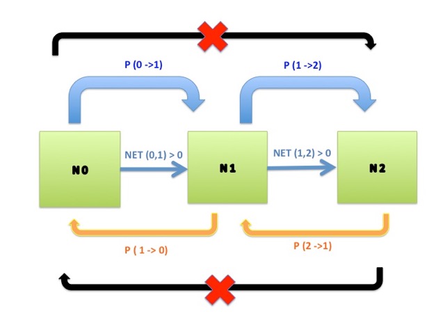
We will consider a system in which all agents have confidence 1. Updating is asynchronous and interactions appear through random mixing. We note that the constraint imposed by the confidence implies that agents with beliefs 0 and 2 never influence each other even if they meet (see Figure 1). Therefore any encounter that modifies beliefs necessarily involves an agent with belief 1.
Model and notation
Let N be the number of agents. Because we are interested in asymptotics with respect to population size we want to be able to compare the states of systems of different size. To this effect, we define a state as an \(n_0,n_1,n_2\in Q^3\) such that \(n_0+n_1+n_2=1\). The triplet \(n_0,n_1,n_2\) represents the fractions of the population of agents who have beliefs 0, 1 and 2 respectively, which we refer to as "level 0", "level 1", and "level 2" agents. In a population of size N, the number of level i agents is then given by Nni. We will only consider values of N for which Nni is a natural number for i= 1, 2, 3. Note that Nni = Ni(0), the initial number of agents in level i.
We now need to describe how the beliefs of the agents evolve over time due to the interactions. We thus introduce random variables whose evolution can be identified with that of the belief evolution as long as the latter has not reached a steady state.
For i= 0,2, we define the quantities Ni(t) in the following way:
| $$ N_2(t)= N_2(0)+\sum_{s=0}^{s=t-1}A_s{\bf 1}_{Z_s=1} \nonumber \\ N_0(t)=N_0(0)-\sum_{s=0}^{s=t-1}B_s{\bf 1}_{Z_s=-1} \nonumber $$ |
Since there is a total of N agents, we deduce that the number of agents who hold belief 1 is given by
| $$ N_1(t)=N-N_0(t)-N_2(t)$$ |
The factors that determine the belief evolution are as follows: The variables (\(Z_s)_{s\ge 1}\) can be seen as determining whether the agent with belief 1 encounters an agent with belief 2 (\(Z_s=1)\), 0 (\(Z_s=-1)\), or an agent who also has belief 1 (\(Z_s=0)\) at time \(s\ge 1\). The probability of encountering an agent with belief 1 or 0 depends on the proportion of agents in the population: \(N_0(t)=N_0(0)-\sum_{s=0}^{s=t-1}B_s{\bf 1}_{Z_s=-1}\), \(P(Z_t=1)=\frac{N_2(t)}{N}\), \(P(Z_t=-1)=\frac{N_0(t)}{N}\). When two agents with belief 1 meet, nobody changes beliefs.
Suppose that \(Z_s=1\), or in other words that an encounter occurs between an agent with belief 1 and an agent with belief 2. There are three possible outcomes of this encounter which we model by a random variable As that takes the values 1, 0, -1 with probability \(p_2,1-p_2-p_1, p_1\). The case As=1: the agent with belief 1 is persuaded by the agent with belief 2 and changes his belief to 2, thus becoming a level 2 agent, the case As= -1: the agent with belief 2 is persuaded by the agent with belief 1 and changes his belief to 1, and finally the case As= 0: neither agent manages to convince the other one and no one changes his belief. Similarly, when \(Z_s=-1\), an encounter occurs between a level 1 agent and a level 0 agent. The three possible outcomes are determined by a random variable Bs which takes the values 1, 0, -1 with probability \(p_1,1-p_1-p_0, p_0\). Similarly, if Bs= 1, the level 0 agent changes his belief to 1 if Bs= -1, the level 1 agent changes his belief to 0. The probability pi is equal to the probability that the agent at level i influences his partner times the probability that he is chosen to be the leading agent in the interaction (this probability is always 1/2 since all the agents have the same confidence).
Since we want to capture the fact that better knowledge of the environment makes an agent more convincing, we will require that \(p_2>p_1>p_0\), or equivalently that \((E(A)=p_2-p_1)>0\) and \((E(B)=p_1-p_0)>0\). This corresponds to the fact that the expected evolution of beliefs favors a transition towards better knowledge.
The evolution of beliefs occurs at each step in time and is modeled with the two sequences of variables \((A_s)_{s\ge 1}\), and \((B_s)_{s\ge 1}\). The variables in the sequence \((A_s)_{s\ge 1}\) are independent and identically distributed. The variables in the sequence \((B_s)_{s\ge 1}\) are also independent and identically distributed (the laws of the variables in the two sequences are not necessarily the same). Moreover, the variables in the sequence \((A_s)_{s\ge 1}\) are independent from those in the sequence \((B_s)_{s\ge 1}\).
We note that the system \(N_0(t),N_2(t)\) which evolves as a function of the random variables \((Z_s)_s\), and \((A_s)_{s\ge 1}\), \((B_s)_{s\ge 1}\)is well defined without reference to \(N_1(t\)) but it only coincides with that of the belief evolution as long as \(N_1(t\))>0.
Asymptotic behavior and results
Having defined above the quantities \((N_0(t), N_1(t),N_2(t))\) which represent the number of agents with belief 0, 1 and 2, we will be interested in the steady states that this system can reach. A steady state is a state which is permanent in the sense that the beliefs will not evolve any more. There are four possible steady states: \(N_i(t)=N\) for some i= 0, 1, 2. This corresponds to a situation where all agents hold identical beliefs i. The fourth absorbing state is that where there are no longer any agents with belief 1. In this case, communication barriers will prevent influence between the agents with belief 0 and 2. This absorbing state occurs when \(N_1(t)=N-N_0(t)-N_2(t)\)=0. An absorbing state of this type can be written as \((N_0(\infty),0, N_2(\infty))\) such that \(N_0(\infty)+N_2(\infty)=1\). We note there cannot be any other type of steady states because if there are still agents who have belief 1 and at least one agent whose belief is different from 1, an encounter can occur and with positive probability the agent whose belief is not 1 changes his belief to 1 in contradiction with the assumption that we were in a steady state.
As said before we assume that better knowledge of the environment translates into greater ability to convince. In other words the expected evolution of beliefs makes it more likely to move from 0 to 1 and from 1 to 2 than in the reverse direction. In other words \(E(A)>0\) and \(E(B)>0\). For this reason, it is easy to see that when the number of agents N is large, absorbing states will be either \(N_2(\infty)=N\), that is, all agents have learned the true state of the world, or states of the last type where \(N_1(\infty)=0\). The other two states require flows that are in contradiction with expected behavior and are untypical in large populations.
We will begin by showing that without the presence of communication barriers due to the presence of confident agents, with high probability, all the agents in a sufficiently large population will eventually learn the correct state of the environment provided that we start from an initial condition where a positive fraction of agents
know the true state of the world (proof in Appendix). This case can be seen as a benchmark with which we can compare the results we obtain when we introduce confident agents in the influence process. We will show that the presence of confident agents leads to a qualitative difference in the long run outcome. Now, starting from any initial condition where each belief is held by a positive fraction of the population, we reach a steady state where a significant proportion of the agents are permanently stuck with their incorrect beliefs.
Proposition 1. For any initial condition such that \(n_0>0\), \(n_2>0\), and for any \(\delta>0\), there exists \(N_0\) such that if \(N>N_0\), the probability is at least \(1-\delta\) that \(N_0(\infty)\ge (1-\frac{E(B)}{N})^{\beta N+N\delta}>0\).
Moreover, we can analyze how different model parameters influence the fraction of agents who remain in a state of low knowledge:
Proposition 2. \(N_0(\infty)/N\) the asymptotic fraction of agents that remain in level 0 is:
- increasing in \(n_0\) (assuming that an increase in \(n_0\) is compensated by a decrease in \(n_1\), holding \(n_2\) constant)
- increasing in \(n_2\) (assuming that an increase in \(n_2\) is compensated by a decrease in \(n_1\), holding \(n_0\) constant)
- increasing in \(E(A)\)
- decreasing in \(E(B)\)
The proof of this proposition can be found in the section on comparative statics at the end of the paper.
The lower bound in the proposition allows us to identify factors that lead to inefficient collective learning. On one hand, we can see that if \(E(A)\) < < \(E(B)\), the number of agents who are asymptotically in a state of low knowledge is close to \(n_0\). In other words, most of the agents who were initially in a state of low knowledge will remain in a state of low knowledge. The lower bound also depends on the initial condition \((n_0,n_1,n_2)\). We note that a higher initial value of knowledge does not necessarily lead to better long run outcomes. For example, \((n_0, n_1-t,n_2+t)\) can lead to worse long run learning than \((n_0,n_1,n_2)\).
Main intuitions behind results
The mechanism that accounts for the described outcome is quite intuitive. Absorbing states where \(N_0(\infty)>0\) occur because there are no longer any agents with belief 1 who ensure the communication. The fact that a positive fraction of agents remain in level 0 is explained by the encounter probabilities alone. Since \(E(B)>0\), there is an expected flow out from level 0. Since encounters occur uniformly at random, eventually the population in level 0 is very small in size whereas that in level 2 has grown outstandingly. The probability of encountering the remaining agents in level 0 is very low. However, there are other important factors that determine whether a larger, non negligible fraction of the population will remain in the low state of knowledge. It is only in this case that we can really say that social learning is inefficient. When E(A) is large compared to E(B) it means that typically the net rate of agents who move from belief 1 to belief 2 is greater than the net rate of moves from 0 to 1. If the number of agents initially in belief 1 is not too large compared to the number of agents in level 0, it is likely that all agents with belief 1 move to belief 2 before most of the agents in belief 0 move to belief 1. Clearly, the long run outcome also depends on the relative sizes of the populations with beliefs 0, 1 and 2. However, the most interesting observation is probably that in the simplified belief environment the fact that agents with correct beliefs are much more convincing does not improve social learning in the population as a whole.
A simulation model based on the analytical model
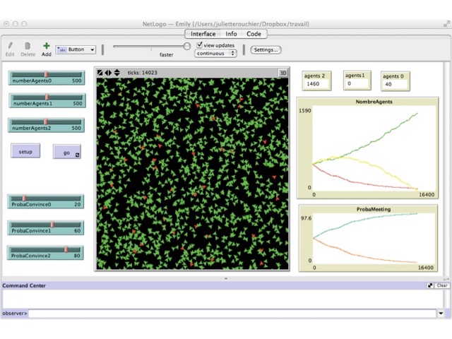
The analytical results we provide are asymptotic, meaning that they are valid when the number of agents and time-steps tend to infinity. It is natural to make such assumptions to obtain analytical results, but it is not necessarily the time scale that is relevant in relation to the socio-environmental dynamics we are dealing with in our story. Hence, we copied the logic of the analytical model into a new simulation model, which greatly simplifies the previous one. The model was written with NetLogo and can be found with a short description at: https://www.openabm.org/model/4756/version/1/view.
At initialization, agents are created and attributed a level of knowledge (0, 1 or 2). Whenever an encounter between two agents occurs, each of the agents is drawn to be the leader with probability 1/2. The probability (expressed in what follows as a percentage) that the leader influences the follower is then respectively P0, P1, and P2 for agents of knowledge level 0, 1 and 2. We have \(\frac{P0}{2}=p_0\), \(\frac{P1}{2}=p_1\),\(\frac{ P_2}{2}=p_2\), since the transition probabilities defined in the previous sections are given by the probability that each agent is chosen to be the influencer in the encounter times the probability that he actually influences his partner.
The value of the probability to influence is initialized for each level of knowledge, with the constraint that P0 < P1 < P2, since the most knowledgeable agents are those who influence most as described in both previous models. At each time-step, a level 1 agent is chosen and another agent is picked among level 0 and level 2 agents. One of these two agents is chosen randomly as the leader and we determine, using the associated probability, whether he will influence the other agent. If so, the level of knowledge of the influenced agent changes and becomes the same as that of the leader. The simulation stops when no agent of level 1 remains.
In our dynamics, we do not consider meetings between agents that cannot result in a change of opinion for the agents involved, and since we are in a setting with agents who are self-assured (with communication barrier), a level 1 agent is always chosen first.
What we can expect from the simulation, if we assume that it will behave like the analytical model although we now consider a finite population size, is that:
- We keep many agents in the bad knowledge situation when \((P1 - P0) < (P2 - P1)\)
- If we fix the probabilities, it is better to have the initial \(N_2(0)\) not too high compared to \(N_1(0)\), so as to achieve complete learning.
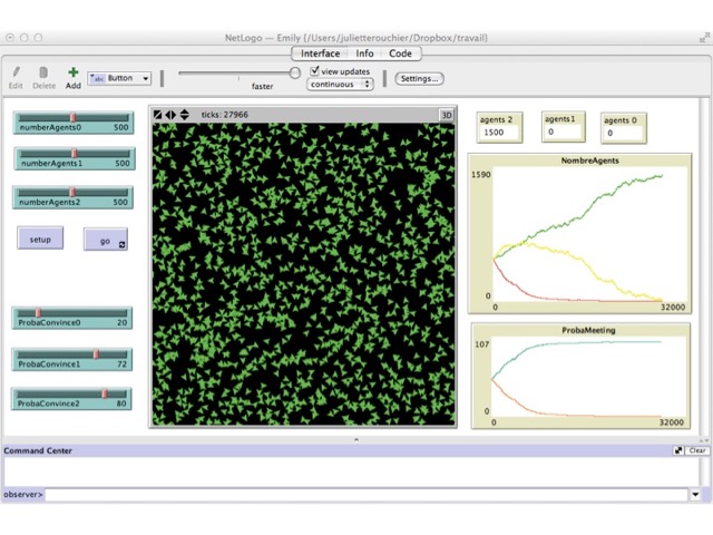
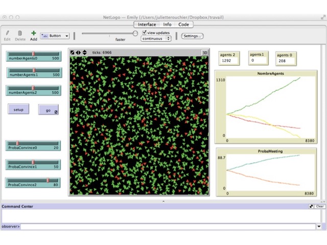
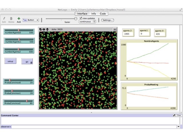
Varying probabilities
We first ran simulations with 500 agents at each level, varying the probability to influence. The results can be observed in Figures 2 to Figure 5. In the first setting, both differences between probabilities are equal, and thus level 0 agents who do not learn are numerous (Figure 3). In the case when P2 - P1 = 8 and P2 - P1 = 52, all level 0 agents get to level 2 in almost all simulations (Figure 2); whereas if the difference of probability is the same, with value 30, there are still many level 0 agents at the end of the simulation (Figure 3). Of course, if P2 - P1 > P1 - P0 then there are still many level 0 agents at the end (e.g. Figure 4). Finally, it is only when the difference (P1 - P0) - (P2 - P1) is really large that we can bring all agents to learn in most simulations. In all other cases, there are still agents of level $0$ at the end (e.g. Figure 2, 4 and 5). These results are summarized in Table 1, where an increase in P2 holding other probabilities constant reduces global learning, and an increase in P1 holding other probabilities constant increases global learning. What we can conclude from this set of simulations, is that our first expectation is realized in the simulation model.
| Values of P1 | 15 | 20 | 30 | 40 | 50 | 60 | 70 |
|---|---|---|---|---|---|---|---|
| P2 = 70 | 469.31 | 429.31 | 326.88 | 193.15 | 60.6 | 3.09 | |
| P2 = 80 | 472.3 | 442.28 | 360.1 | 255.62 | 132.05 | 34.82 | 1 |
| P2 = 90 | 475.9 | 450.34 | 383.3 | 293.58 | 188.15 | 87.49 | 19.29 |
Hence we can see that the result holds, and that the most important element is the relative ability to convince of agents at level 2 and 1.
| Initial value | Initial value | Initial value | non-knowledgeable agents |
|---|---|---|---|
| N0 = 500 | N1 = 500 | N2 = 500 | 3.5 |
| N0 = 200 | N1 = 800 | N2 = 500 | 0.8 |
| N0 = 800 | N1 = 500 | N2 = 200 | 5.6 |
| N0 = 500 | N1 = 800 | N2 = 200 | 0.2 |
| N0 = 500 | N1 = 200 | N2 = 800 | 21.4 |
Initial number of agents
In the second set of simulations, we kept probabilities unchanged, using what was previously a favorable setting with P0 = 20%, P1 = 70% and P2 = 80% and we vary the initial number of each group of agents. We first keep 500 level 2 agents and vary the other values, and then keep the number of level 0 agents at 500 and vary the others, while keeping their sum constantly equal to 1000.
These results show that the influence of the initial number of agents in each category is also important in a finite population, and follows the rule that has been established in the analytical model, even when the time steps and number of agents are finite.
Some aspects of these global results are rather counter-intuitive, such as the fact that better transmission of good information leads to worse collective learning. This can be observed in the former table where, for increasing values of P2 we also produce a final number of non-knowledgeable agents which increases. Here, dyadic good learning does not imply collective good learning.
Discussion
The new analysis we conducted, re-writing the idea of our model with a new methodology, confirms the main result of the previously published work.
If we define an individual with high confidence as having difficulty learning from those whose beliefs are too different from his own, then the presence of overconfident agents, who believe that they are correct when they are not, does have a significant negative impact on the level of collective learning.
In this context, which gives rise to a communication barrier between agents with different beliefs, the result had been shown in a complex environment, through simulation. Here we show that it holds asymptotically (very large number of agents and repeated interactions) with a simplified representation of the environment. By using the analytical model to build new simulations with a moderate number of agents, we can also check that this simplified model can be used in contexts that can be interpreted as real-life situations, where convergence occurs in a population of reasonable size and after a reasonable number of pairwise interactions.
The mechanism we identified in this study can be explained in a simple way: agents refuse to communicate with others when beliefs are too far apart. Initially "moderate" (moderately knowledgeable) agents ensure interactions between the informed and the ignorant. However these agents eventually adopt the views of the better informed agents since the latter are more convincing. However a group of agents with very low knowledge is left behind and no intermediate agents are left to ensure communication between them and the informed agents. In some sense, all those whose initial beliefs are not too incorrect in the beginning will learn the true state quickly but the others are left behind. It is interesting to note that the rapid initial success of the informed agents may not be efficient for learning in the population as a whole in the long run. The moderately informed agents learn quickly but this leaves the mistaken agents isolated and creates polarization.
It is interesting to note that what causes the bad learning dynamics is mainly the lack of moderately knowledgeable agents, rather than the lack of highly informed agents, or a high number of agents whose initial beliefs are incorrect. It is not necessarily good for global outcomes that perfectly knowledgeable agents exert a strong influence, and thus that the power of persuasion increases too much with the quality of knowledge.
We can express sufficient conditions for bad collective learning:
- if the initial fraction of agents with an intermediate level of knowledge is small
- the likelihood of persuading ones partner is convex with respect to the level of knowledge
The analytical study of a simplified model is what allowed us to make this mechanism visible, and thus to show that communication barriers is a major issue in the management of collective learning. However, the result about convexity which holds in the simplified model does not necessarily hold in a more complex representation of the belief environment. Indeed, as can be seen in Rouchier & Tanimura (2012), the convexity and concavity do not produce straightforward properties, since increasing the convexity by starting from a linear reaction to the environment does reduce learning, but moving from the linear to the concave case does as well. In our complex setting the best learning occurs when the success of transmission of good information is linear in the quality of this information. Intuitively, in the new setting this can be seen as corresponding to a situation where (P1 - P0) = (P2 - P1), but it is rather clear that it is not possible to translate the representation in one model to the other as easily. Hence, the main result can be explained and proved, but the same is not true for the more detailed properties of the original model. Indeed, one has to bear in mind that the main difference between RT2012 and this analytical model is the notion of "correct" and "incorrect" beliefs. In the complex setting, there is one way to be correct, but many ways to be incorrect.
As is usually the case in a model-to-model comparison process, the analytical model is very different from the initial simulation model, and requires a completely new way of phrasing the problem. This second step can be made only when the simulation model has provided us with some intuitive hypothesis that can then be verified in a much simpler setting. Developing a new model which conserves important features of the original one but is more tractable is an interesting creative challenge which also requires finding appropriate analytical methods for studying models and problems originated in agent based modeling. In our case, where there is randomness in the encounters that occur and in their outcomes, it was natural to take a probabilistic approach, focusing on "typical" outcomes in the long run.
Appendix: Proofs
No communication barrier random walk
Let us first consider the case where there are no communication barriers. In this situation, dynamics end in one of three possible states \(N_0(\infty)=N\), \(N_1(\infty)=N\) or \(N_2(\infty)=N\). Let us show that if \(N\) is sufficiently large, with high probability we reach an outcome where all agents learn the true state of the world, i.e. the last case. We will be interested in \(N_2(t)\) the number of agents with a correct belief. Let us consider only the transition of agents in and out of level 2. We disregard whether the agents who are not in level 2 are in level 0 or level 1. When an encounter occurs between an agent in level 2 and an agent in level 1, the probability that the agent in level 1 moves to level 2 is \(p_2\), the probability that an agent in level 2 moves to level 1 is \(p_1\) and the probability that nobody moves is \(1-(p_1+p_2)\). Conditioning on the event that someone moves, the probability of moving to level 2 is \(p_2/(p_1+p_2)\) and the probability of moving to level 1 is \(p_1/(p_1+p_2)\). (The steps where nobody moves affect convergence time but not the movement of the dynamics and can be ignored). Similarly we can consider the probability of moving from level 0 to level 2 and conversely, when a movement occurs, the probability of moving to level 2 is \(p_2/(p_0+p_2)\) and that of moving to level 0 is \(p_0/(p_0+p_2)\). The probability of moving to level 2 is higher for the agents at level 0 than for those at level 1. Thus the probability that an agent in level 0 or level 1 moves to level 2, in a step where movement actually occurs, is greater than \(p_2/(p_1+p_2)\). Let us consider the modified dynamics where any agent in level 0 or 1 moves to level 2 with probability \(P_R=:p_2/(p_1+p_2)\) and the probability that an agent in level 2 moves to level 0 or 1 (we do not care which one it is) is \(P_L=:1-P_R\). Under the modified dynamics \(N_2(t)\) defines a simple one-dimensional random walk on \(Z\) with probabilities \((P_R, 1-P_R)\) where \(P_R>1/2\). Let us identify the initial position \(n_2N\) with the position 0 in the random walk on \(Z\). The event \(N_2(t)=N(n_1+n_0)\) means that all agents are in level 2, and the even \(N_2(t)=0\) is the event where all agents are in level 0 or 1 in the steady state. Define the stopping times \(\tau_{n_1+n_0}=inf\{t>0\vert N_2(t)=(n_1+n_0)N\}\) and \(\tau_{-n_2}=inf\{t>0\vert N_2(t)=-Nn_2 \}\). The absorbing state is \(N_2(\infty)=N\) exactly when the random walk hits \(Nn_1+Nn_0\) before it hits \(-Nn_2\), or in other words when \(\tau_{n_1+n_0}<\tau_{-n_2}\). Now this is a well known gamblers' ruin problem. Since \((\frac{1-P_R}{P_R})<1\), we have
| $$P(\tau_{n_1+n_0}<\tau_{-n_2})=\frac{(\frac{1-P_R}{P_R})^{Nn_2}-1}{(\frac{1-P_R}{P_R})^{N(n_0+n_1)}-1}\to_{n\to \infty}1.$$ | (1) |
Proposition 3. The probability that we reach a steady state with only level 2 agents is bounded below by
| $$P(\tau_{n_1+n_0}<\tau_{-n_2})=\frac{(\frac{1-P_R}{P_R})^{Nn_2}-1}{(\frac{1-P_R}{P_R})^{N(n_0+n_1)}-1}\to_{n\to \infty}1.$$ | (2) |
Communication barrier
Let us give an expression for the expected value of the number of agents in level \(2\) at time \(t+1\) given then number of agents in level 2 at time \(t\). The number changes only if an agent in level 1 meets an agent in level 2. The probability that this occurs is \(N_2(t)/N\). When such a meeting occurs, the number of agents in level 2 increases by 1 with probability \(p_2\) and decreases by 1 with probability \(p_1\), with \(p_2-p_1=:E(A)\). Therefore, we have \(E[N_2(t+1)\vert F_t]=\frac{N_2(t)}{N}E(A)+N_2(t)=(1+\frac{E(A)}{N})N_2(t).\) Similarly, the agents in level 0 evolve according to: \(E[N_0(t+1)\vert F_t]=\frac{-N_0(t)}{N}E(B)+N_0(t)=(1-\frac{E(B)}{N})N_0(t).\)
Consequently, we can define two martingales \((\tilde{N}_2(t))_{t\ge 0}=(\frac{N_2(t)}{1+E(A)/N)^t})_{t\ge 0}\) and \((\tilde{N}_0(t))_{t\ge 0}=(\frac{N_0(t)}{1-E(B)/N)^t})_{t\ge 0}\).
We will now define events that say essentially that the sequences behave typically at time \(t\):
| $$E_2(t)=: N(n_2-\epsilon)(1+\frac{E(A)}{N})^t< N_2(t)< N(n_2+\epsilon)(1+\frac{E(A)}{N})^t$$ | (3) |
| $$E_0(t)=: N(n_0-\epsilon)(1-\frac{E(B)}{N})^t< N_0(t)\le N(n_0+\epsilon)(1-\frac{E(B)}{N})^t$$ | (4) |
Note that we can also write
| $$E_2(t)=: \tilde{N}_2(0)-N\epsilon< \tilde{N}_2(t)< \tilde{N}_2(0)+N\epsilon$$ | (5) |
| $$E_0(t)=:\tilde{N}_0(0)-N\epsilon< \tilde{N}_0(t)< \tilde{N}_0(0)+N\epsilon.$$ | (6) |
To obtain an upper bound on the probability that the sequences are not typical in this sense, we will apply the Azuma-Hoeffding inequality which we recall:
Lemma 1. (Azuma-Hoeffding inequality) Let \((X_t)_{t\ge 0}\) be a martingale with bounded differences: \(\vert X_{t+1}-X_t\vert \le t_k\) then
\(P(\vert X_t-X_0\vert a)\le exp(\frac{-a^2}{2\sum_{l=1}^{l=t}(t_l)^2}).\)
Applying the Azuma inequality to \((\tilde{N}_2(t))_{t\ge 0}\) and \((\tilde{N}_0(t))_{t\ge 0}\), we can take \(t_k=1\) for all \(k\), since \(N_2(t)\) and \(N_0(t)\) change by at most one element in a period. We have by the Azuma inequality:
| $$P(E_2^C)=:P( \tilde{N}_2(0)-N\epsilon< \tilde{N}_2(t)< \tilde{N}_2(0)+N\epsilon)\le 2exp(\frac{-(N\epsilon)^2}{2t})$$ | (7) |
| $$P(E_0^C)=:P(\tilde{N}_0(0)-N\epsilon< \tilde{N}_0(t)< \tilde{N}_0(0)+N\epsilon)\le 2exp(\frac{-(N\epsilon)^2}{2t}).$$ | (8) |
Our dynamics enter a steady state when there are no longer any agents in level 1. This is the event \(N_1(t)=\emptyset \iff N_2(t)+N_0(t)\ge N\). We will be interested in the date at which this occurs. If the process behaved exactly according to expectation, the date would be \(T\) defined as
| $$T=:inf\{t>0\vert N(n_2)(1+\frac{E(A)}{N})^t)+N(n_0)(1-\frac{E(B)}{N})^t)=N\}.$$ | (9) |
We note that for sufficiently large \(N\), \(T\le \frac{ln(1/n_2)}{ln(1+E(A)/N)}\le -2ln(n_2)N/E(A)=:\beta N.\)
If the process behaves \(\epsilon\)-typically, the earliest date at which \(N_1(t)=\emptyset\) can occur is
| $$T_m=:min\{t>0\vert N(n_2+\epsilon)(1+\frac{E(A)}{N})^t)+N(n_0+\epsilon)(1-\frac{E(B)}{N})^t)=N\}$$ | (10) |
| $$T_M=:min\{t>0\vert N(n_2-\epsilon)(1+\frac{E(A)}{N})^t)+N(n_0-\epsilon)(1-\frac{E(B)}{N})^t)=N\}.$$ | (11) |
Define \(K=:min\{t\vert N_1(t)=\emptyset\}\). If the process is \(\epsilon\)-typical until \(T_M\), we will have \(K\in [T_m,T_M]\). By continuity, for any \(\delta>0\), we can find an \(\epsilon>0\) such that \([T_m,T_M]\subset [T-N\delta, T+N\delta]\). Consequently, we will have \(K \in [T-N\delta, T+N\delta]\) if the process is typical until \(T_M\). It is in fact sufficient to show that the process is typical between \(\hat{T}=min\{n_0N,n_2N\}\) and \(T_M\). Indeed, we cannot have \(N_1(t)=0\) before \(\hat{T}\), moreover, if the process is typical for all \(t=\hat{T},..,T_M\), we cannot have \(N_2(t)=0\) before \(T_M\). Moreover, \(T_M\le T+\delta N\le (\beta+1)N\).
Let \(\epsilon>0\) defined as above be fixed. We bound the probability that the process is typical for \(t=\hat{T},...,(\beta+1)N\).
| $$P(\bigcap_{t=\hat{T}}^{t=T_M}(E_2(t),E_0(t)))=1-P(\bigcup_{t=\hat{T}}^{t=T_M}(E_2(t),E_0(t))^C)\ge 1-\sum_{t=\hat{T}}^{t=T_M}P((E_2(t),E_0(t))^C)$$ | (12) |
| $$\ge (T_M-\hat{T})N2exp(\frac{-(\hat{T}\epsilon)^2}{2T_M}).$$ | (13) |
Where we use the fact that \(P((E_2(t),E_0(t))^C)\le 2exp(\frac{-\hat{T}\epsilon)^2}{2T_M})\) for all \(t\ge T_M\). Since \(\hat{T}=min\{n_1N,n_2N\}\le T_M \le N \beta\), we can then find \(N_0\) such that for \(N>N_0\), we have \((T_M-\hat{T})N2exp(\frac{-(n_1N\epsilon)^2}{2n_1N})<\delta\). We obtain:
Proposition 4. Let
| $$T=:inf\{t>0\vert N(n_2)(1+\frac{E(A)}{N})^t)+N(n_0)(1-\frac{E(B)}{N})^t)=N\}$$ | (14) |
- \(K\in [T-N\delta, T+N\delta]\)
- \(N_0(\infty)=N_0(K)\ge (n_0-\epsilon)(1-\frac{E(B)}{N})^{T+\delta}\ge (1-\frac{E(B)}{N})^{\beta N+N\delta}>0\).
Remark 1. The above proposition implies that for large population sizes, with high probability the asymptotic proportion of agents in level 0 is positive. Indeed under the stated conditions, \(T\le \beta N\), with \(\beta=-ln(n_2)/E(A)\) and thus
\(N_0(\infty)=(1-\frac{E(B)}{N})^{T+N\delta}\ge (1-\frac{E(B)}{N})^{\beta N+N\delta}>0.\)
Comparative statics
Proposition 1 establishes the fact that the presence of communication barriers leads to a qualitative difference in the steady state: the fraction of level 0 agents is positive. However, the fraction can be very small. In practice, whether or not learning is successful depends on the model parameters. In this section, we will analyze how each of the parameters \(n_0, n_1,n_2\) and \(E(A), E(B)\) impacts the steady state fraction of level 0 agents. We can choose \(\delta\) so that the steady state fraction \(N_0(\infty)\) is arbitrarily close to \(n_0(1+\frac{E(B)}{N})^T\). Therefore, we will analyze the impact of the parameters on the quantity \(n_0(1-\frac{E(B)}{N})^T\). Moreover, since we have \(T=O(N)\) and \(N\) is large, we can use the approximations \((1-\frac{E(B)}{N})^{tN}=exp(-E(B)t)\) and \((1+\frac{E(A)}{N})^{tN}=exp(E(A)t)\). The quantity \(T(n_0,n_2, E(A),E(B))\) is then defined through as an implicit function by \(g((T, n_0,n_2, E(A),E(B))=0\), where \(g((T, n_0,n_2, E(A),E(B))=: n_2exp(E(A)t)+n_0exp(-E(B)t)-1\). We have \(\frac{\delta T}{\delta q}=\frac{-\delta g/ \delta q}{\delta g/ \delta T}\). Now consider as a function of \(t\), \(g(t)=n_2exp(E(A)t)+n_0exp(-E(B)t)\). We have \(\frac{\delta g}{ \delta t}=:g^{'}(t)=n_2E(A)exp(E(A)t))-n_0E(B)exp(-E(B)t))\). Let us show that \(g^{'}(t)\ge 0\) when \(g(t)=1\). It is readily verified that \(g^{''}(t)>0\). Suppose that \(g^{'}(0)<0\), which is possible for some parameter values. Then there exists \(v>0\) such that \(g^{'}(t)\le 0\) iff \(t\le v\). Now, \(g(0)=n_2+n_0-1<0\). Since \(g(t)\) is decreasing on \([0,v]\), \(g(t)< g(0)< 0\) for all \(t\le v\). Thus \(g(\bar{t})=0\) implies \(\bar{t}>v\) which implies \(g^{'}(\bar{t})>0\). By the implicit function theorem, the differential of \(T\) with respect to \(q\) is \(\frac{\delta T}{\delta q}=\frac{-\delta g/ \delta q}{\delta g/ \delta T}\), where we have established the positivity of \(\delta g/ \delta T\).
The asymptotic fraction of agents in level 0 is \(H(n_0, E(B), T)=n_0exp(-E(B)T)\). We study how this function depends on the different parameters.
| $$\frac{\delta N_1}{\delta n_0}=H^{'}_{n_0}\frac{\delta T}{\delta n_0} = exp(-E(B)t)+\frac{n_0E(B)(exp(-E(B)t))^2}{ \delta g/ \delta T}>0$$ | (15) |
| $$\frac{\delta N_1}{\delta n_2}=H^{'}_{n_2}\frac{\delta T}{\delta n_2}=\frac{n_0E(B)exp(E(A)t)exp(-E(B)t)}{\delta g/ \delta T }>0$$ | (16) |
| $$\frac{\delta N_1}{\delta E(A)}=H^{'}_{E(A)}\frac{\delta T}{\delta E(A)}=\frac{n_0E(B)exp(-E(B))n_2texp(E(A)t)}{ \delta g/ \delta T}>0$$ | (17) |
| $$\frac{\delta N_1}{\delta E(B)}=H^{'}_{E(B)}\frac{\delta T}{\delta E(B)}=\frac{-n_0E(B)exp(-E(B))n_0texp(-E(B)t)}{ \delta g/ \delta T}<0$$ | (18) |
From this analysis, we obtain the comparative statics results given in Proposition 2.
In the proposition, we assume that we are holding \(n_2\) constant and increase \(n_0\) by decreasing \(n_1\). and similarly when we change \(n_2\). We also note that the quantities \(E(A)\) and \(E(B)\) are related due to the fact that \(E(A)=p_2-p_1\) and \(E(B)=p_1-p_0\). If \(E(A)>>E(B)\), we must have \(p_2-p_1>>p_1-p_0\) which corresponds to a learning probability that is convex with respect to knowledge. Conversely if \(E(B)>>E(A)\), the learning probability is concave with respect to knowledge. Thus in the dynamics we consider, social learning is more successful with a concave success probability.
References
AXELROD, R. (1997). The dissemination of culture. A model with local convergence and global polarization. Journal of Conflict Resolution, 41(2), pp, 203–226.
CECCONI, F., Campennì, M., Andrighetto, G. & Conte, R. (2010). What do agent-based and equation-based modelling tell us about social conventions: The clash between ABM and EBM in a congestion game framework. Journal of Artificial Societies and Social Simulation, 13(1), 6: https://www.jasss.org/13/1/6.html. [doi:10.18564/jasss.1585]
CIOFFI-REVILLA, C. & Gotts, N. (2003). Comparative analysis of agent-based social simulations: Geosim and Fearlus models. Journal of Artificial Societies and Social Simulation, 6(4), 10: https://www.jasss.org/6/4/10.html
DEFFUANT, G., Weisbuch, G., Amblard, F. & Faure, T. (2013). The results of Meadows and Cliff are wrong because they compute indicator y before model convergence. Journal of Artificial Societies and Social Simulation, 16(1), 11: https://www.jasss.org/16/1/11.html [doi:10.18564/jasss.2211]
EDMONDS, B. & Hales, D. (2003). Replication, replication and replication: Some hard lessons from model alignment.Journal of Artificial Societies and Social Simulation, 6(4), 11: https://www.jasss.org/6/4/11.html.
EDWARDS, M., Huet, S., Goreaud, F. & Deffuant, G. (2003). Comparing an individual-based model of behaviour diffusion with its mean field aggregate approximation. Journal of Artificial Societies and Social Simulation, 6(4), 9: https://www.jasss.org/6/4/9.html.
GRAZZINI, J. (2012). Analysis of the emergent properties: Stationarity and ergodicity. Journal of Artificial Societies and Social Simulation, 15(2), 7: https://www.jasss.org/15/2/7.html. [doi:10.18564/jasss.1929]
HALES, D., Rouchier, J. & Edmonds, B. (2003). Model-to-model analysis. Journal of Artificial Societies and Social Simulation, 6(4), 5: https://www.jasss.org/6/4/5.html.
JANSSEN, M. A., Alessa, N., Barton, M., Bergin, S. & Lee, A. (2008). Towards a community framework for agent-based modelling. Journal of Artificial Societies and Social Simulation, 11(2), 6: https://www.jasss.org/11/3/6.html.
KLÜVER, J. & Stoica, C. (2003). Simulations of group dynamics with different models. Journal of Artificial Societies and Social Simulation, 6(4), 8: https://www.jasss.org/6/4/8.html.
MACY, M. & Sato, Y. (2008). Reply to Will and Hegselmann. Journal of Artificial Societies and Social Simulation, 11(4), 11: https://www.jasss.org/11/4/11.html.
MEADOWS, M. & Cliff, D. (2012). Reexamining the relative agreement model of opinion dynamics. Journal of Artificial Societies and Social Simulation, 15(4), 4: https://www.jasss.org/15/4/4.html. [doi:10.18564/jasss.2083]
POLHILL, G., Parker, D., Brown, D. & Grimm, V. (2007). 'Using the odd protocol for comparing three agent-based social simulation models of land use change'. In C. Cioffi-Revilla, G. Podhill, J. Rouchier & K. Takadama (Eds.), Model to Model 3. Marseille: GREQAM.
POLHILL, J. G., Izquierdo, L. R. & Gotts, N. M. (2005). The ghost in the model (and other effects of floating point arithmetic). Journal of Artificial Societies and Social Simulation, 8(1), 5: https://www.jasss.org/8/1/5.html.
POLHILL, J. G., Parker, D., Brown, D. & Grimm, V. (2008). Using the ODD protocol for describing three agent-based social simulation models of land-use change. Journal of Artificial Societies and Social Simulation, 11(2), 3: https://www.jasss.org/11/2/3.html.
ROUCHIER, J. (2003). Reimplementation of a multi-agent model aimed at sustaining experimental economic research: the case of simulations with emerging speculation. Journal of Artificial Societies and Social Simulation, 6(4), 7: https://www.jasss.org/6/4/7.html.
ROUCHIER, J., Cioffi-Revilla, C., Podhill, G. & Takadama, K. (2008). Progress in model-to-model analysis. Journal of Artificial Societies and Social Simulation, 11(2), 8: https://www.jasss.org/11/2/8.html.
ROUCHIER, J. & Shiina, H. (2007). 'Learning and belief dissemination through co-action'. In S. Takahashi, D. Sallach & J. Rouchier (Eds.), Advancing Social Simulation. The First World Congress. Tokyo: Springer, pp. 225–236.
ROUCHIER, J. & Tanimura, E. (2012). When overconfident agents slow down collective learning. Simulation, 88(1), pp. 33–49 [doi:10.1177/0037549711428948]
SILVERMAN, E., Bijak, J., Hilton, J., Cao, V. D. & Noble, J. (2013). When demography met social simulation: A tale of two modelling approaches. Journal of Artificial Societies and Social Simulation, 16(4), 9: https://www.jasss.org/16/4/9.html. [doi:10.18564/jasss.2327]
URBIG, D., Lorenz, J. & Herzberg, H. (2008). Opinion dynamics: the effect of the number of peers met at once. Journal of Artificial Societies and Social Simulation, 11(2), 4: https://www.jasss.org/11/2/4.html.
VILA, X. (2008). A model-to-model analysis of bertrand competition. Journal of Artificial Societies and Social Simulation, 11(2), 11: https://www.jasss.org/11/2/11.html.
WILENSKY, U. & Rand, W. (2007). Making models match: Replicating an agent-based model. Journal of Artificial Societies and Social Simulation, 10(4), 2: https://www.jasss.org/10/4/2.html.
WILL, O. (2009). Resolving a replication that failed: News on the Macy and Sato model. Journal of Artificial Societies and Social Simulation, 12(4), 11: https://www.jasss.org/12/4/11.html.
WILL, O. & Hegselmann, R. (2008). A replication that failed: On the computational model in Michael W. Macy and Yoshimichi Sato: Trust, cooperation and market formation in the U.S. and Japan. Proceedings of the National Academy of Sciences, May 2002’. Journal of Artificial Societies and Social Simulation, 11(3), 3: https://www.jasss.org/11/3/3.html.