
Michael Barber, Philippe Blanchard, Eva Buchinger, Bruno Cessac and Ludwig Streit (2006)
Expectation-Driven Interaction: a Model Based on Luhmann's Contingency Approach
Journal of Artificial Societies and Social Simulation
vol. 9, no. 4
<https://www.jasss.org/9/4/5.html>
For information about citing this article, click here
Received: 29-Aug-2005 Accepted: 14-Sep-2006 Published: 31-Oct-2006

 Abstract
These concepts will be integrated in a model which explores interaction strategies using different types of interconnected memories. The interconnectedness of the memories is a precondition for obtaining agents “capable of acting.”
That information be measured by entropy is, after all, natural when we remember that information, in communication theory, is associated with the amount of freedom of choice we have in constructing messages. Thus for a communication source one can say, just as he would also say it of a thermodynamic ensemble, ‘This situation is highly organized, it is not characterized by a large degree of randomness or of choice—that is to say, the information (or the entropy) is low.’ (Weaver 1949, pg. 13)
By information we mean an event that selects system states. This is possible only for structures that delimit and presort possibilities. Information presupposes structure, yet is not itself a structure, but rather an event that actualizes the use of structures.... Time itself, in other words, demands that meaning and information must be distinguished, although all meaning reproduction occurs via information (and to this extent can be called information processing), and all information has meaning.... a history of meaning has already consolidated structures that we treat as self-evident today. (Luhmann 1995, pg. 67)
According to social systems theory, the historically evolved general meaning structure is represented on the micro level (i.e., psychic systems, agent level) in the form of the personal life-world (Luhmann 1995, pg. 70). A personal meaning-world represents a structurally pre-selected repertoire of possible references. Although the repertoire of possibilities is limited, selection is necessary to produce information. Meaning structure provides a mental map for selection but does not replace it. All together, the one is not possible without the other—information production presupposes meaning structure and the actualization of meaning is done by information production.
Within the present version of the ME model, agents do not have the option to reject a message or to refuse to answer. Their “freedom” is incorporated in the process of message selection. Agents can be distinguished by the number of messages they are able to use and by their selection strategies. The ongoing exchange of messages creates an interaction sequence with a limited—but possibly high—number of steps.
In social systems, expectations are the temporal form in which structures develop. But as structures of social systems expectations acquire social relevance and thus suitability only if, on their part, they can be anticipated. Only in this way can situations with double contingency be ordered. Expectations must become reflexive: it must be able to relate to itself, not only in the sense of a diffuse accompanying consciousness but so that it knows it is anticipated as anticipating. This is how expectation can order a social field that includes more than one participant. Ego must be able to anticipate what alter anticipates of him to make his own anticipations and behavior agree with alter’s anticipation. (Luhmann 1995, pg. 303)
 .
.
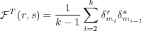
 the joint probability that agent A maintains at time
  ,
estimating the likelihood that agent B will transmit a message
,
estimating the likelihood that agent B will transmit a message  to which
agent A will respond with a message
to which
agent A will respond with a message  . Second, we use the conditional
probability
. Second, we use the conditional
probability  , showing the likelihood of agent A responding with
message
, showing the likelihood of agent A responding with
message  given that agent B has already transmitted message
  . Finally, we
use the marginal probability
. Finally, we
use the marginal probability  , showing the likelihood of agent A responding
with message
, showing the likelihood of agent A responding
with message  regardless of what message agent B sends. These three
probabilities are related by
regardless of what message agent B sends. These three
probabilities are related by
 | (1) |
 | (2) |
We use similar notation for all the memories (and other probabilities) in this work.
 is a time-dependent memory that agent A
maintains about interactions with agent B, where agent B provides the stimulus
is a time-dependent memory that agent A
maintains about interactions with agent B, where agent B provides the stimulus  to which agent A gives response
  . During the course of interaction with agent B,
the corresponding ego memory is continuously updated based on the notion that the
ego memory derives from the relative frequency of stimulus-response pairs.
In general, an agent will have a distinct ego memory for each of the other
agents.
. During the course of interaction with agent B,
the corresponding ego memory is continuously updated based on the notion that the
ego memory derives from the relative frequency of stimulus-response pairs.
In general, an agent will have a distinct ego memory for each of the other
agents.
 (as
well as agent B’s counterpart
(as
well as agent B’s counterpart  ) is undefined. As agents A and B interact
through time
) is undefined. As agents A and B interact
through time  , they together produce a message sequence
  .
Assuming that agent B has sent the first message, one view of the sequence is that
agent B has provided a sequence of stimuli
.
Assuming that agent B has sent the first message, one view of the sequence is that
agent B has provided a sequence of stimuli  to which
agent A has provided a corresponding set of responses
to which
agent A has provided a corresponding set of responses  .
If agent A began the communication, the first message could be dropped
from the communication sequence; similarly, if agent B provided the final
message, this “unanswered stimulus” could be dropped from the communication
sequence.
.
If agent A began the communication, the first message could be dropped
from the communication sequence; similarly, if agent B provided the final
message, this “unanswered stimulus” could be dropped from the communication
sequence.
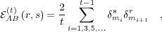 | (3) |
for all  and
and  . In Eq. (3), we assume that the memory has an infinite
capacity, able to exactly treat any number of stimulus-response pairs. A
natural and desirable modification is to consider memories with a finite
capacity.
. In Eq. (3), we assume that the memory has an infinite
capacity, able to exactly treat any number of stimulus-response pairs. A
natural and desirable modification is to consider memories with a finite
capacity.
 , with a value from the interval
![[0,1]](5/communication24x.png) , such that the ego memory is calculated as
, such that the ego memory is calculated as
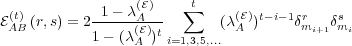 | (4) |
for all  and
and  . The memory of a particular message transmission decays
exponentially.
. The memory of a particular message transmission decays
exponentially.
 is analogous to the ego memory, but with the roles
of sender and receiver reversed. Thus,
is analogous to the ego memory, but with the roles
of sender and receiver reversed. Thus,  is the memory that agent A
maintains about message exchanges with agent B, where agent A provides the
stimulus
is the memory that agent A
maintains about message exchanges with agent B, where agent A provides the
stimulus  to which agent B gives response
  . The procedure for calculating the
alter memory directly parallels that for the ego memory, except that the messages
sent by agent A are now identified as the stimuli and the messages sent by agent B
are now identified as the responses. The calculation otherwise proceeds as
before, including making use of a forgetting parameter
. The procedure for calculating the
alter memory directly parallels that for the ego memory, except that the messages
sent by agent A are now identified as the stimuli and the messages sent by agent B
are now identified as the responses. The calculation otherwise proceeds as
before, including making use of a forgetting parameter  for the alter
memory.
for the alter
memory.
 , agent A tracks the responses of
agent B to stimuli from agent A. This is exactly what agent B tracks in its
ego memory
, agent A tracks the responses of
agent B to stimuli from agent A. This is exactly what agent B tracks in its
ego memory  . Thus, the memories of the two agents are related
by
. Thus, the memories of the two agents are related
by
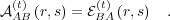 | (5) |
However, Eq. (5) holds only if the agent memories are both infinite or  .
The corresponding relation
.
The corresponding relation 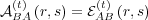 holds as well when the memories
are both infinite or
holds as well when the memories
are both infinite or  .
.
 of agent A is, like the ego and
alter memories, represented as a joint distribution, but there are many marked
differences. Significantly, the response disposition is not associated with another
particular agent, but instead shows what the agent brings to all interactions. In
particular, the response disposition can act like a general data bank applicable to any
other agent. Further, the response disposition changes more slowly. Instead, the
update occurs after the interaction sequences. In this work, we hold the response
dispositions fixed, so we defer discussion of a possible update rule for the response
disposition to section 5.1.
of agent A is, like the ego and
alter memories, represented as a joint distribution, but there are many marked
differences. Significantly, the response disposition is not associated with another
particular agent, but instead shows what the agent brings to all interactions. In
particular, the response disposition can act like a general data bank applicable to any
other agent. Further, the response disposition changes more slowly. Instead, the
update occurs after the interaction sequences. In this work, we hold the response
dispositions fixed, so we defer discussion of a possible update rule for the response
disposition to section 5.1.
 . Thus, what
responses agent A has given to agent B in the past will be favored in the
future, so that there is a continual pressure for an agent to be consistent in its
responses.
. Thus, what
responses agent A has given to agent B in the past will be favored in the
future, so that there is a continual pressure for an agent to be consistent in its
responses.
 that it could send. This
corresponds to calculating the entropy based on the conditional alter memory
that it could send. This
corresponds to calculating the entropy based on the conditional alter memory
 , yielding
![[ ]
H A(t) (⋅ ∣ r) = - ∑ A(t) (r′ ∣ r)log A(t) (r′ ∣ r) .
A∣B r′ A∣B nS A∣B](5/communication43x.png) | (6) |
The base of the logarithm is traditionally taken as 2, measuring the entropy in bits,
but in this work we take the base to be  , the number of different messages. With
this choice, the entropy take on values from the interval
, the number of different messages. With
this choice, the entropy take on values from the interval ![[0,1]](5/communication45x.png) , regardless of the
number of messages.
, regardless of the
number of messages.
![[ ]
H A(t) (⋅ ∣ r)
A ∣B](5/communication46x.png) is closely related to the expectation-certainty
from Dittrich et al. (2003). Note that all possible messages
is closely related to the expectation-certainty
from Dittrich et al. (2003). Note that all possible messages  are considered, so
that agent A may send a message to agent B that is highly unlikely based on a
just-received stimulus. Thus, we expect that resolving uncertainty and satisfying
expectations will come into conflict.
are considered, so
that agent A may send a message to agent B that is highly unlikely based on a
just-received stimulus. Thus, we expect that resolving uncertainty and satisfying
expectations will come into conflict.
![(t) (A) (A) (t) (A) [ (t) ] (A)1--
UA∣B(r ∣ s) ∝ c1 QA (r ∣ s)+c 2 EA∣B(r ∣ s)+c 3 H A A∣B (⋅ ∣ r)+c 4 nS .](5/communication48x.png) | (7) |
The parameters c(A) 1 , c(A) 2 , and c(A) 3 reflect the relative importance of the three factors discussed above, while c(A) 4 is an offset that provides a randomizing element. The randomizing element provides a mechanism for, e.g., introducing novel messages or transitions. It also plays an important role on mathematical grounds (see the appendix).
 to be negative. A positive
  corresponds to agent A favoring messages that lead to unpredictable responses, while
a negative
corresponds to agent A favoring messages that lead to unpredictable responses, while
a negative  corresponds to agent A “inhibiting” messages that lead to
unpredictable response, hence favoring messages leading to predictable responses.
When
corresponds to agent A “inhibiting” messages that lead to
unpredictable response, hence favoring messages leading to predictable responses.
When  is negative, Eq. (7) could become negative. Since
  is a
probability, we deal with this negative-value case by setting it to zero whenever
Eq. (7) gives a negative value.
is a
probability, we deal with this negative-value case by setting it to zero whenever
Eq. (7) gives a negative value.
 is changed from a positive to a negative value. This is illustrated
mathematically in the appendix and numerically in section 4.2. We do, in fact,
observe a sharp transition in the entropy of the alter and ego memories of the agent
(measuring the average uncertainty in their response) near
is changed from a positive to a negative value. This is illustrated
mathematically in the appendix and numerically in section 4.2. We do, in fact,
observe a sharp transition in the entropy of the alter and ego memories of the agent
(measuring the average uncertainty in their response) near  . Note however
that the transition depends also on the other parameters and does not necessarily
occur exactly at
. Note however
that the transition depends also on the other parameters and does not necessarily
occur exactly at  . This is discussed in the appendix. The transition is
reminiscent of what Dittrich et al. call the appearance of social order, though our
model is different, especially because of the response disposition which plays a crucial
role in the transition.
. This is discussed in the appendix. The transition is
reminiscent of what Dittrich et al. call the appearance of social order, though our
model is different, especially because of the response disposition which plays a crucial
role in the transition.
 ,
,  ,
,  , and
, and  allows the
transition probabilities used by Dittrich et al. to be constructed as a special case of
Eq. (7). In particular, their parameters
allows the
transition probabilities used by Dittrich et al. to be constructed as a special case of
Eq. (7). In particular, their parameters  ,
,  , and
, and  are related to the ones
used here by
are related to the ones
used here by
 | (8) |
 | (9) |
 | (10) |
 | (11) |
 from the response disposition
 , using
 | (12) |
With the marginal probability of initial messages  and the conditional
probability for responses
and the conditional
probability for responses  , stochastic simulations of the model system
are relatively straightforward to implement programmatically.
, stochastic simulations of the model system
are relatively straightforward to implement programmatically.
We address these briefly below. Many other questions are, of course, possible.
 through
 .
.
 changes its sign. Simulations demonstrating the transition are presented in
section 4.2.3.
changes its sign. Simulations demonstrating the transition are presented in
section 4.2.3.
 is near zero. We assign to the asymptotic state a set of
observables measuring the quality of the interaction according to different
criteria.
is near zero. We assign to the asymptotic state a set of
observables measuring the quality of the interaction according to different
criteria.
![[0,1]](5/communication74x.png) and normalizing the total
probability. With random response dispositions of this sort, the contribution to the
agent behavior is complex but unique to each agent. A second type of agent has its
behavior restricted to a subset of the possibilities, never producing certain messages.
A response disposition for this type of agent, when presented as a matrix, can be
expressed as a block structure, such as in Fig. 1. A third and final type of agent
response disposition that we consider has a banded structure, as in Fig. 7, allowing
the agent to transmit any message, but with restricted transitions between
them.
and normalizing the total
probability. With random response dispositions of this sort, the contribution to the
agent behavior is complex but unique to each agent. A second type of agent has its
behavior restricted to a subset of the possibilities, never producing certain messages.
A response disposition for this type of agent, when presented as a matrix, can be
expressed as a block structure, such as in Fig. 1. A third and final type of agent
response disposition that we consider has a banded structure, as in Fig. 7, allowing
the agent to transmit any message, but with restricted transitions between
them.
|
| (a) agent A |
|
| (b) agent B |
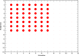
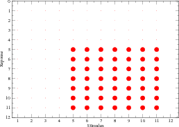
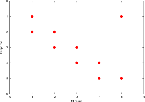
| Figure 1. Block-structured response dispositions. The size of the circle is proportional to the value of the corresponding entry |
 | (13) |
The constraint is in no way fundamental, but is useful for graphical presentation of simulation results.
 . The elements of the probability matrices are shown as circles whose
sizes are proportional to the value of the matrix elements, with the sum of the values
equal to one.
. The elements of the probability matrices are shown as circles whose
sizes are proportional to the value of the matrix elements, with the sum of the values
equal to one.
 block where the
elements have uniform values of
block where the
elements have uniform values of  , while all other elements are zero. The blocks
for the two agents have a non-zero overlap. The subdomain for agent A deals with
messages 1 through 7, while that for agent B deals with messages 5 through 11.
Thus, if agent B provides a stimulus from
, while all other elements are zero. The blocks
for the two agents have a non-zero overlap. The subdomain for agent A deals with
messages 1 through 7, while that for agent B deals with messages 5 through 11.
Thus, if agent B provides a stimulus from  , agent A responds with a
message from
, agent A responds with a
message from  with equiprobability. The coefficients
  and
and  are both set to
  . These terms are useful to handle the response of the
agent when the stimulus is “unknown” (i.e., it is not in the appropriate
block). In such a case, the agent responds to any stimulus message with equal
likelihood.
. These terms are useful to handle the response of the
agent when the stimulus is “unknown” (i.e., it is not in the appropriate
block). In such a case, the agent responds to any stimulus message with equal
likelihood.
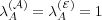
 to the first mode of
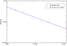
  (see section A.5). We measure the distance between these two vectors at the end of
the simulation. The distance tends to zero when the number of interaction sequences
(see section A.5). We measure the distance between these two vectors at the end of
the simulation. The distance tends to zero when the number of interaction sequences
 increases, but it decreases slowly, like
  (as expected from the central limit
theorem). An example is presented in Fig. 2 for
(as expected from the central limit
theorem). An example is presented in Fig. 2 for  and
and
 .
.
|
Figure 2. Evolution of the distance between the vector  (t)
A (t)
A  and the first
mode of U(∞)
A∣BU(∞)
B∣A as the number of interaction sequences increases and the first
mode of U(∞)
A∣BU(∞)
B∣A as the number of interaction sequences increases
|
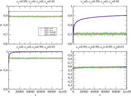
 ,
,
 ,
,  ,
and
,
and  . For each case, we first
examined the convergence to the asymptotic regime. We show the evolution of the
joint entropy in Fig. 3. This allows us to estimate the time needed to reach the
asymptotic regime.
. For each case, we first
examined the convergence to the asymptotic regime. We show the evolution of the
joint entropy in Fig. 3. This allows us to estimate the time needed to reach the
asymptotic regime.
 . In
Fig. 5, we show the values with a finite memory (
. In
Fig. 5, we show the values with a finite memory ( ,
corresponding to a characteristic time scale of approximately 100 steps). Our main
observations are:
,
corresponding to a characteristic time scale of approximately 100 steps). Our main
observations are:
 . The responses of each agent
are essentially determined by its response disposition. The asymptotic
behavior is given by
. The responses of each agent
are essentially determined by its response disposition. The asymptotic
behavior is given by  and
and  , the first modes of the matrices
 and
and  , respectively. Fig. 2 shows indeed the convergence
to this state. The asymptotic values of the alter and ego memories are given
by
, respectively. Fig. 2 shows indeed the convergence
to this state. The asymptotic values of the alter and ego memories are given
by  and
and  The memory matrices have a “blockwise”
structure with a block of maximal probability corresponding to the stimuli
known by both agents.
The memory matrices have a “blockwise”
structure with a block of maximal probability corresponding to the stimuli
known by both agents.
 . The response of each agent
is essentially determined by its ego memory. As expected, the maximal
variance is observed for this case. Indeed, there are long transient
corresponding to metastable states and there are many such states.
. The response of each agent
is essentially determined by its ego memory. As expected, the maximal
variance is observed for this case. Indeed, there are long transient
corresponding to metastable states and there are many such states.
 . The response of each agent
is essentially determined by its alter memory, and the probability is higher
for selecting messages that induce responses with high uncertainty. Again,
the asymptotic state is the state of maximal entropy.
. The response of each agent
is essentially determined by its alter memory, and the probability is higher
for selecting messages that induce responses with high uncertainty. Again,
the asymptotic state is the state of maximal entropy.
 . The response of
each agent is essentially determined by its alter memory, but the
probability is lower for selecting messages that induce responses with high
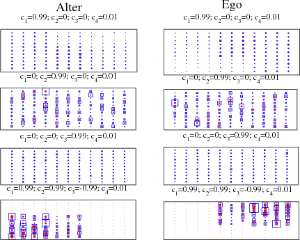
uncertainty. The asymptotic memories have an interesting structure. The
alter and ego memories have block structures like that of both agents’
response dispositions, but translated in the set of messages exchanged
(contrast Fig. 1 and the bottom row of Fig. 5). The effect is clear if we
keep in mind that, for agent A’s ego memory, the stimulus is always given
by agent B, while for agent A’s alter memory, the stimulus is always given
by agent A.
. The response of
each agent is essentially determined by its alter memory, but the
probability is lower for selecting messages that induce responses with high
uncertainty. The asymptotic memories have an interesting structure. The
alter and ego memories have block structures like that of both agents’
response dispositions, but translated in the set of messages exchanged
(contrast Fig. 1 and the bottom row of Fig. 5). The effect is clear if we
keep in mind that, for agent A’s ego memory, the stimulus is always given
by agent B, while for agent A’s alter memory, the stimulus is always given
by agent A.
|
Figure 3. Evolution of the joint entropy of alter and ego memory with infinite
(λ( ) = λ( ) = λ( ) = 1) and finite (λ() = λ() = 0.99) memories ) = 1) and finite (λ() = λ() = 0.99) memories
|
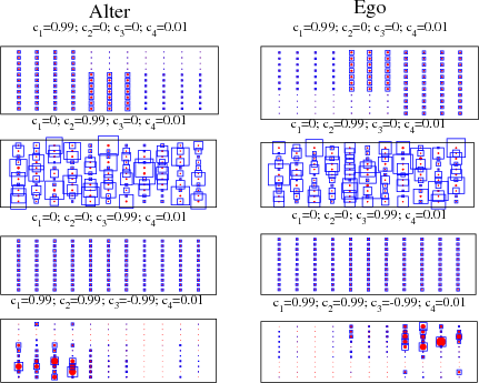
|
| Figure 4. Average asymptotic memories for agent A after 128000 steps, with infinite memories. The matrices shown here are calculated by averaging over 10 initial conditions. The sizes of the red circles are proportional to the corresponding matrix elements, while the sizes of the blue squares are proportional to the mean square deviations |
|
|
Figure 5. Average asymptotic memories for agent A after 128000 steps, with
finite memories (λ() = λ() = 0.99). The matrices shown here are calculated by
averaging over 10 initial conditions. The sizes of the red circles are proportional
to the corresponding matrix elements, while the sizes of the blue squares are
proportional to the mean square deviations
|
 are set to different, extremal values. The role of
the forgetting parameter is also important. In some sense, the asymptotic matrices
whose structure are the closest to the block structure of the response dispositions are
the matrices in the bottom row of Fig. 5, where the agent are able to “forget.” There
is a higher contrast between the blocks seen in the corresponding row of Fig. 4 when
are set to different, extremal values. The role of
the forgetting parameter is also important. In some sense, the asymptotic matrices
whose structure are the closest to the block structure of the response dispositions are
the matrices in the bottom row of Fig. 5, where the agent are able to “forget.” There
is a higher contrast between the blocks seen in the corresponding row of Fig. 4 when
 .
.
 and
and  vary.
Note, however, that the general situation where agents A and B have different
coefficients requires investigations in an 8 dimensional space. Even if we impose
constraints of the form in Eq. (13), this only reduces the parameter space to
6 dimensions. A full investigation of the space of parameters is therefore
beyond the scope of this paper and will be done in a separate work. To
produce a manageable parameter space, we focus here on the situation where
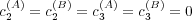
agents A and B have identical coefficients and where
vary.
Note, however, that the general situation where agents A and B have different
coefficients requires investigations in an 8 dimensional space. Even if we impose
constraints of the form in Eq. (13), this only reduces the parameter space to
6 dimensions. A full investigation of the space of parameters is therefore
beyond the scope of this paper and will be done in a separate work. To
produce a manageable parameter space, we focus here on the situation where
agents A and B have identical coefficients and where  is fixed to a
small value (
is fixed to a
small value ( ). The number of messages exchanged by the agents is
 .
.
 space, we simulate interaction with response
dispositions of both agents selected randomly (see section 4.2.1 for details). We
conduct 10000 successive interaction sequences of length 11 for each pair of agents. In
each sequence, the agent that transmit the first message is selected at random.
Therefore we have a total exchange of 110000 messages.
space, we simulate interaction with response
dispositions of both agents selected randomly (see section 4.2.1 for details). We
conduct 10000 successive interaction sequences of length 11 for each pair of agents. In
each sequence, the agent that transmit the first message is selected at random.
Therefore we have a total exchange of 110000 messages.
 and
and
 .
.
 and
and  both vary
in the interval
both vary
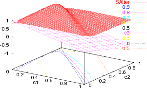
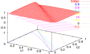
in the interval ![[0,0.99]](5/communication118x.png) . Consequently,
. Consequently, ![c3 ∈ [- 0.99 : 0.99]](5/communication119x.png) . There is an
abrupt change in the entropy close to the line
. There is an
abrupt change in the entropy close to the line  (
( ).
The transition does not occur exactly at said line, but depends on
).
The transition does not occur exactly at said line, but depends on  and
and
 .
.
 parameter space. Note, however, that the transition is not
precisely at
parameter space. Note, however, that the transition is not
precisely at  , but rather to a more complex line as discussed in the
appendix.
, but rather to a more complex line as discussed in the
appendix.
|
(a) Infinite memory (λ( ) = λ( ) = λ( ) = 1) ) = 1)
|
|
|
(b) Finite memory (λ() = λ() = 0.99).
|
| Figure 6. Asymptotic joint entropy for alter memory of agent A, with (a) infinite memories and (b) finite memories. The plane represents c3 = 0. The colored lines in the c1-c2 plane are level lines for the joint entropy, while the black line shows where the c3 = 0 plane intersects the c1-c2 plane |
 messages. The first type of agent is a “teacher” agent A that has relatively
simple behavior. Its response disposition has a banded structure, shown in Fig. 7.
The teacher agent has a fixed behavior dependent only upon its response disposition
(
messages. The first type of agent is a “teacher” agent A that has relatively
simple behavior. Its response disposition has a banded structure, shown in Fig. 7.
The teacher agent has a fixed behavior dependent only upon its response disposition
( ). The values of
  and
and  are irrelevant, since the
alter and ego memories contribute nothing.
are irrelevant, since the
alter and ego memories contribute nothing.
|
| Figure 7. Banded response disposition. The size of the circle is proportional to the value of the corresponding entry |
 and
and  to investigate
the effects of the various parameters. We take the memories to be infinite,
to investigate
the effects of the various parameters. We take the memories to be infinite,
 .
.
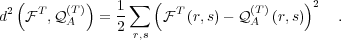
 , defined by
 | (14) |
The value of  always lies in the interval
 ![[0,1]](5/communication136x.png) .
.
 , which
depends only on memories of agent A and is therefore in principle available to
agent A. This reveals an interesting asymmetry in the system; the teacher
agent A has an ability to assess the interaction that the student agent B
lacks.
, which
depends only on memories of agent A and is therefore in principle available to
agent A. This reveals an interesting asymmetry in the system; the teacher
agent A has an ability to assess the interaction that the student agent B
lacks.
 messages are exchanged before the target distance is
reached, the rate is simply
messages are exchanged before the target distance is
reached, the rate is simply  . The simulated interaction can be limited to a
finite number of exchanges with the rate set to zero if the target is not reached
during the simulation.
. The simulated interaction can be limited to a
finite number of exchanges with the rate set to zero if the target is not reached
during the simulation.
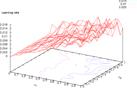
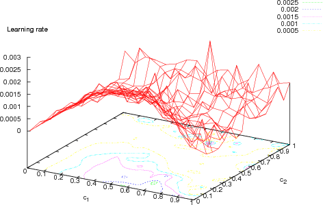
 is shown. For this
case, the rates have a simple structure, generally proceeding more rapidly
with
is shown. For this
case, the rates have a simple structure, generally proceeding more rapidly
with  . In contrast, Fig. 8(b) presents quite different results based
on a target distance of
. In contrast, Fig. 8(b) presents quite different results based
on a target distance of  , with more complex structure to the rates.
In this latter case, the highest rates occur with
, with more complex structure to the rates.
In this latter case, the highest rates occur with  . We note that
inclusion of the response disposition is crucial in this scenario. In particular,
the rate of change goes to zero if the student agent suppresses its response
disposition.
. We note that
inclusion of the response disposition is crucial in this scenario. In particular,
the rate of change goes to zero if the student agent suppresses its response
disposition.
|
(a) Target distance 
|
|
(b) Target distance 
|
| Figure 8. Rates of change for the alter memory of the student agent approaching the response disposition of the teacher agent. The colored lines in the c1-c2 plane are level lines for the rates |
 has been presented as time
independent. To generalize this, we number the interaction sequences and add an
index to the response disposition to indicate the sequence number, giving
has been presented as time
independent. To generalize this, we number the interaction sequences and add an
index to the response disposition to indicate the sequence number, giving
 .
.
 messages labeled
 , we find
  , the empirical frequency of message pairs for
interaction sequence
, the empirical frequency of message pairs for
interaction sequence  , using
 | (15) |
for all  and
and  . Note that Eq. (15) utilizes all of the messages exchanged,
regardless of whether the agent ego and alter memories have infinite memories (i.e.,
. Note that Eq. (15) utilizes all of the messages exchanged,
regardless of whether the agent ego and alter memories have infinite memories (i.e.,
 ) or undergo “forgetting” (i.e.,
  or
or  ). This is
due to an assumed period of reflection in which details of the interaction can be
considered at greater length.
). This is
due to an assumed period of reflection in which details of the interaction can be
considered at greater length.
 ) and that expressed by the
response disposition of the agents. A small distance is indicative of relevance or
usefulness of the interaction sequence to the agent, while a great distance suggests
that the interaction sequence is, e.g., purely speculative or impractical.
) and that expressed by the
response disposition of the agents. A small distance is indicative of relevance or
usefulness of the interaction sequence to the agent, while a great distance suggests
that the interaction sequence is, e.g., purely speculative or impractical.
 using
using
 | (16) |
Since  and
and  are both probability distributions, the distance
 must lie in the interval
 ![[0,1]](5/communication162x.png) The value of the distance must be
below an acceptance threshold
The value of the distance must be
below an acceptance threshold  that reflects the absorbative capacity of
agent A, limiting what interaction sequences agent A accepts.
that reflects the absorbative capacity of
agent A, limiting what interaction sequences agent A accepts.
 | (17) |
where the update rate  is in the interval
 ![[0,1]](5/communication166x.png) . The update rule in Eq. (17) is
applied if and only if
. The update rule in Eq. (17) is
applied if and only if  .
.
 be the affinity that
agent X has for agent Y , we set the probability that agent X and agent Y
interact to be proportional to
be the affinity that
agent X has for agent Y , we set the probability that agent X and agent Y
interact to be proportional to  (the product is appropriate because
the affinities need not be symmetric). A pair of interacting agents can then
be chosen based on the combined affinities of all the agents present in the
system.
(the product is appropriate because
the affinities need not be symmetric). A pair of interacting agents can then
be chosen based on the combined affinities of all the agents present in the
system.
 . For example, agents can be
constructed to predominately interact with other agents they assess as similar by
defining
. For example, agents can be
constructed to predominately interact with other agents they assess as similar by
defining
 | (18) |
where  is a settable parameter and
  is the distance defined in Eq. (14).
The affinities can be viewed as the weights in a graph describing the agent
network.
is the distance defined in Eq. (14).
The affinities can be viewed as the weights in a graph describing the agent
network.
2For long interaction sequences, the response disposition could be updated periodically—but less frequently than the ego and alter memories—during the sequence.
 is the conditional probability that agent A selects
message
is the conditional probability that agent A selects
message  at time
  given that agent B selected
  at time
  . It is given
by Eq. (7),
. It is given
by Eq. (7),
![( )
(t) 1 (A) (A) (t) (A) [ (t) ] c(4A)
UA∣B(r ∣ s) =-(t)- c1 QA (r ∣ s)+ c2 EA∣B(r ∣ s)+ c3 H AA∣B(⋅ ∣ r) +-nS ,
NA ∣B](5/communication179x.png) | (19) |
where ![[ (t) ]
H AA∣B(⋅ ∣ r)](5/communication180x.png) is
is
![[ ] n∑S ( )
H A(t) (⋅ ∣ r) = - A(t) (r′ ∣ r)logn A(t) (r′ ∣ r) .
A∣B r′=1 A∣B S A∣B](5/communication181x.png) | (20) |
Note that this term does not depend on  . The normalization factor
  is
given by
is
given by
![( )
(t) (A) n∑S [ (t) ]
NA∣B = 1+ c3 H AA∣B (⋅ ∣ r) - 1
r=1](5/communication184x.png) | (21) |
and does not depend on time when  . Moreover,
 | (22) |
It will be useful in the following to write  in matrix form, so
that
in matrix form, so
that
![(t) -1---( (A) (A) (t) (A) [ (t) ] (A) )
U A∣B = N (t) c1 QA + c2 EA∣B + c3 H A A∣B + c4 S ,
A∣B](5/communication188x.png) | (23) |
with a corresponding equation for the  . The matrix
  is the uniform
conditional probability, with the form
is the uniform
conditional probability, with the form
 | (24) |
We use the notation ![[ (t) ]
H AA∣B](5/communication192x.png) for the matrix with the
for the matrix with the  element given by
![[ ]
H A(t) (⋅ ∣ r)
A∣B](5/communication194x.png) .
.
 and agent A selects at
even times. When it does not harm the clarity of the expressions, we will
drop the subscripts labeling the agents from the transition probabilities
and call
and agent A selects at
even times. When it does not harm the clarity of the expressions, we will
drop the subscripts labeling the agents from the transition probabilities
and call  the transition matrix at time
  , with the convention that
 and
and  . Where possible, we will further simplify
the presentation by focusing on just one of the agents, with the argument
for the other determined by a straightforward exchange of the roles of the
agents.
. Where possible, we will further simplify
the presentation by focusing on just one of the agents, with the argument
for the other determined by a straightforward exchange of the roles of the
agents.
 the probability that the relevant agent selects message
  at time
 . The evolution of
  is determined by a one parameter family of (time
dependent) transition matrices, like in Markov chains. However, the evolution is not
Markovian since the transition matrices depend on the entire past history (see
section A.3).
is determined by a one parameter family of (time
dependent) transition matrices, like in Markov chains. However, the evolution is not
Markovian since the transition matrices depend on the entire past history (see
section A.3).
 an infinite message exchange
sequence where
an infinite message exchange
sequence where  is the
  -th exchanged symbol. The probability that the
finite subsequence
-th exchanged symbol. The probability that the
finite subsequence  has been selected is given by
![Prob[mt, mt-1,...,m2, m1] =
U(t)(mt ∣ mt-1)U(t- 1)(mt- 1 ∣ mt-2)...U(2)(m2 ∣ m1)P(1)(m1) .(25)](5/communication208x.png) | (25) |
Thus,
 | (26) |
Since agent B selects the initial message, we have  .
As well, the joint probability of the sequential messages
.
As well, the joint probability of the sequential messages  and
and  is
is
![(t) (t- 1)
Prob [mt,mt -1] = U (mt ∣ mt-1)P (mt- 1) .](5/communication213x.png) | (27) |
 depend on the response dispositions. Therefore one can at
most expect statistical statements referring to some probability measure on the space
of response disposition matrices (recall that the selection probability for the first
message is also determined by the response disposition). We therefore need to
consider statistical averages to characterize the typical behavior of the model for
fixed values of the coefficients
depend on the response dispositions. Therefore one can at
most expect statistical statements referring to some probability measure on the space
of response disposition matrices (recall that the selection probability for the first
message is also determined by the response disposition). We therefore need to
consider statistical averages to characterize the typical behavior of the model for
fixed values of the coefficients  and
and  .
.
 depends on the entire past (via the ego and
alter memories). In the case where
depends on the entire past (via the ego and
alter memories). In the case where  , the ME model is basically
a Markov process and it can be handled with the standard results in the
field.
, the ME model is basically
a Markov process and it can be handled with the standard results in the
field.
 where
where  is the set of messages. The
corresponding sigma algebra
is the set of messages. The
corresponding sigma algebra  is constructed as usual with the cylinder sets. In
the ME model the transition probabilities corresponding to a given agent are
determined via the knowledge of the sequence of message pairs (second order
approach), but the following construction holds for an
is constructed as usual with the cylinder sets. In
the ME model the transition probabilities corresponding to a given agent are
determined via the knowledge of the sequence of message pairs (second order
approach), but the following construction holds for an  -th order approach,
 , where the transition probabilities depends on a sequence of
  -tuples. If
 is a message sequence, we denote by
  the
sequence of pairs
the
sequence of pairs  . Denote by
 , where
  . We construct a family of conditional
probabilities given by
. We construct a family of conditional
probabilities given by
![[ ] [ ] ( [ ])
P ωt = (r,s)∣ωt-11 = c1Q(r,s)+c2E ωt = (r,s)∣ωt1-1 +c3H A ⋅ ∣ ωt-1 1 (r)+c4](5/communication230x.png) | (28) |
for  , where
![t-1
E [ω = (r,s)∣ωt-1]= 1∑ χ(ω = (r,s)) ,
t 1 tk=1 k](5/communication232x.png) | (29) |
with  being the indicatrix function (
![A [⋅ ∣ ωt-1]
1](5/communication234x.png) has the same form, see
section 3.3.1). For
has the same form, see
section 3.3.1). For  the initial pair
  is drawn using the response
disposition as described in the text. Call the corresponding initial probability
is drawn using the response
disposition as described in the text. Call the corresponding initial probability
 .
.
![[ m n ] n [ n+1] [ m -1]
P ωn+1∣ω1 = P [ωn+1∣ω1]P ωn+2∣ω1 ...P ωm∣ω1](5/communication238x.png) | (30) |
and,  ,
,
![∑ [ m- 1 ] [ m+l m-1] [ m+l ]
m-1P ω1 ∣ω1 P ωm ∣ω1 = P ωm ∣ω1 .
ω1](5/communication240x.png) | (31) |
From this relation, we can define a probability on the cylinders  by
by
![[ m+l] ∑ [ m+l ]
P ωm = P ωm ∣ω1 μ(ω1) .
ω1](5/communication242x.png) | (32) |
This measure extends then on the space of trajectories  by Kolmogorov’s
theorem. It depends on the probability
by Kolmogorov’s
theorem. It depends on the probability  of choice for the first symbol (hence it
depends on the response disposition of the starting agent). A stationary state is then
a shift invariant measure on the set of infinite sequences. We have not yet
been able to find rigorous conditions ensuring the existence of a stationary
state, but some arguments are given below. In the following, we assume this
existence.
of choice for the first symbol (hence it
depends on the response disposition of the starting agent). A stationary state is then
a shift invariant measure on the set of infinite sequences. We have not yet
been able to find rigorous conditions ensuring the existence of a stationary
state, but some arguments are given below. In the following, we assume this
existence.
 and
and  (the case where
 is negative is trickier and is discussed below). When the invariant state is
unique, it is ergodic and in this case the empirical frequencies corresponding to alter
and ego memories converge (almost surely) to a limit corresponding to the marginal
probability
is negative is trickier and is discussed below). When the invariant state is
unique, it is ergodic and in this case the empirical frequencies corresponding to alter
and ego memories converge (almost surely) to a limit corresponding to the marginal
probability ![P[ω]](5/communication248x.png) obtained from Eq. (32). Thus, the transition matrices
obtained from Eq. (32). Thus, the transition matrices  also
converge to a limit.
also
converge to a limit.
 . In this case, the long time behavior of the agent depends on
the initial conditions. A thorough investigation of this point is, however, beyond the
scope of this paper.
. In this case, the long time behavior of the agent depends on
the initial conditions. A thorough investigation of this point is, however, beyond the
scope of this paper.
 . Assume
that the
. Assume
that the  converge to a limit. Then, since the
  are conditional
probabilities, there exists, by the Perron-Frobenius theorem, an eigenvector
associated with an eigenvalue 1, corresponding to a stationary state (the
states may be different for odd and even times). The stationary state is
not necessarily unique. It is unique if there exist a time
are conditional
probabilities, there exists, by the Perron-Frobenius theorem, an eigenvector
associated with an eigenvalue 1, corresponding to a stationary state (the
states may be different for odd and even times). The stationary state is
not necessarily unique. It is unique if there exist a time  such that for
all
such that for
all  the matrices
  are recurrent and aperiodic (ergodic). For
 and
and  , ergodicity is assured by the presence of the matrix
 , which allows transitions from any message to any other message. This
means that for positive
, which allows transitions from any message to any other message. This
means that for positive  the asymptotic behavior of the agents does not
depend on the history (but the transients depend on it, and they can be very
long).
the asymptotic behavior of the agents does not
depend on the history (but the transients depend on it, and they can be very
long).
 , it is possible that some transitions allowed by the matrix
  are
canceled and that the transition matrix
are
canceled and that the transition matrix  loses the recurrence property for
sufficiently large
loses the recurrence property for
sufficiently large  . In such a case, it is not even guaranteed that a stationary
regime exists.
. In such a case, it is not even guaranteed that a stationary
regime exists.
 and especially by the spectral gap (distance between the largest eigenvalue of one and
the second largest eigenvalue). Consequently, studying the statistical properties of the
evolution for the spectrum of the
and especially by the spectral gap (distance between the largest eigenvalue of one and
the second largest eigenvalue). Consequently, studying the statistical properties of the
evolution for the spectrum of the  provides information such as the
rate at which agent A has stabilized its behavior when interacting with
agent B.
provides information such as the
rate at which agent A has stabilized its behavior when interacting with
agent B.
 entering in the
noise term has eigenvalue 0 with multiplicity
entering in the
noise term has eigenvalue 0 with multiplicity  and eigenvalue 1
with multiplicity 1. The eigenvector corresponding to the latter eigenvalue
is
and eigenvalue 1
with multiplicity 1. The eigenvector corresponding to the latter eigenvalue
is
 | (33) |
which is the uniform probability vector, corresponding to maximal entropy.
Consequently,  is a projector onto
  .
.
 . It corresponds
therefore to a matrix where all the entries in a row are equal. More precisely, set
. It corresponds
therefore to a matrix where all the entries in a row are equal. More precisely, set
![[ ]
α(rt)= H A(At)∣B(⋅ ∣ r)](5/communication273x.png) . Then one can write the corresponding matrix in the form
. Then one can write the corresponding matrix in the form
 , where
  is the vector
 | (34) |
and  is the transpose of
  . It follows that the uncertainty term has a 0
eigenvalue with multiplicity
. It follows that the uncertainty term has a 0
eigenvalue with multiplicity  and an eigenvalue
 ![∑nS [ (t) ]
r=1H A A∣B (⋅ ∣ r)](5/communication280x.png) with
corresponding eigenvector
with
corresponding eigenvector  . It is also apparent that, for any probability vector
 , we have
 ![[ ]
H A(tA)∣B P = nSv(At)uTP = v(tA)](5/communication283x.png) .
.
 on
on  is then given by
![P(t+1) = U(t)P(t)
A A ∣B([B ] )
= -1-- c(1A)QA + c(2A)E(At)∣B P(tB)+ c(3A)v(tA)+ c(A4)u . (35)
N (t)](5/communication286x.png) | (35) |
The expression in Eq. (35) warrants several remarks. Recall that all the vectors
above have positive entries. Therefore the noise term  tends to “push”
  in the direction of the vector of maximal entropy, with the effect of increasing the
entropy whatever the initial probability and the value of the coefficients. The
uncertainty term
in the direction of the vector of maximal entropy, with the effect of increasing the
entropy whatever the initial probability and the value of the coefficients. The
uncertainty term  plays a somewhat similar role in the sense that it also has
its image on a particular vector. However, this vector is not static, instead depending
on the evolution via the alter memory. Further, the coefficient
plays a somewhat similar role in the sense that it also has
its image on a particular vector. However, this vector is not static, instead depending
on the evolution via the alter memory. Further, the coefficient  may have either
a positive or a negative value. A positive
may have either
a positive or a negative value. A positive  increases the contribution of
 but a negative
  decreases the contribution. Consequently, we
expect drastic changes in the model evolution when we change the sign of
decreases the contribution. Consequently, we
expect drastic changes in the model evolution when we change the sign of
 —see section 4.2 and especially Fig. 6 for a striking demonstration of these
changes.
—see section 4.2 and especially Fig. 6 for a striking demonstration of these
changes.
 and
and  is easier to handle when an
asymptotic state, not necessarily unique and possibly sample dependent, is reached.
In this case, we must still distinguish between odd times (agent B active) and even
times (agent A active), that is,
is easier to handle when an
asymptotic state, not necessarily unique and possibly sample dependent, is reached.
In this case, we must still distinguish between odd times (agent B active) and even
times (agent A active), that is,  has two accumulation points depending on
whether
has two accumulation points depending on
whether  is odd or even. Call
  the probability that, in the stationary
regime, agent A selects the message
the probability that, in the stationary
regime, agent A selects the message  during interaction with agent B. In the
same way, call
during interaction with agent B. In the
same way, call  the asymptotic joint probability that agent A responds
with message
the asymptotic joint probability that agent A responds
with message  to a stimulus message
  from agent B. Note that, in general,
 , but
, but  and
and
 since each message simultaneous is
both a stimulus and a response.
since each message simultaneous is
both a stimulus and a response.
 converges to a limit
 which is precisely the asymptotic probability of stimulus-response pairs.
Therefore, we have
which is precisely the asymptotic probability of stimulus-response pairs.
Therefore, we have
 | (36) |
 | (37) |
Thus, the  converge to a limit
  , where
![( [ ] )
U(A∞∣)B = --1(∞)- c(1A)QA + c(2A)E(A∞∣)B + c(3A)H A(A∞)∣B +c(4A)S .
NA∣B](5/communication312x.png) | (38) |
From Eq. (27), we have 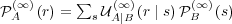 . Hence,
 | (39) |
 | (40) |
and
 | (41) |
 | (42) |
It follows that the asymptotic probability  is an eigenvector of
  corresponding to the eigenvalue 1. We will call this eigenvector the first mode of
the corresponding matrix. Therefore, the marginal ego memory of agent A
converges to the first mode of
corresponding to the eigenvalue 1. We will call this eigenvector the first mode of
the corresponding matrix. Therefore, the marginal ego memory of agent A
converges to the first mode of  . A numerical example is provided in
section 4.2.2.
. A numerical example is provided in
section 4.2.2.
 .
But
.
But  , so
, so
 | (43) |
 | (44) |
Therefore, using the relation  , we have
 | (45) |
 | (46) |
 | (47) |
With this definition, Eqs. (45) and (46) become:
 | (48) |
 | (49) |
We next plug Eq. (49) into Eq. (48). After some manipulation, we obtain
![(∞)
EA∣B (r ∣ s) = [ ]
β(A)Q (r ∣ s)+ β(A)+ β(A)H β(B)Q (⋅ ∣ r)+ β(B)
1 A 4 3 1 B ( 4 [ ] )
∑ β(3B)H E(∞) (⋅ ∣ r′)
- β(3A) (β(1B)QB (r′ ∣ r)+ β(4B))lognS(1 +-(B)---A-∣B-----(B)-)
r′ β1 QB (r′ ∣ r)+ β4
(A) (B)∑ ( (B) ′ (B)) [ (∞) ′]
- β3 β3 lognS β1 QB (r ∣ r) + β4 H EA∣B (⋅ ∣ r)
r′ ( [ ] )
(A) (B)∑ [ (∞) ] β(3B)H E(∞A)∣B (⋅ ∣ r′)
- β3 β3 H EA∣B (⋅ ∣ r′) lognS(1 +-(B)-----′------(B))
r′ β1 QB (r ∣ r)+ β4
, (50)](5/communication326x.png) | (50) |
which uncouples the expression for  from that for
  . In some
sense, Eq. (50) provides a solution of the model with two agents, since it captures
the asymptotic behavior of the ego and alter memories (provided the stationary
regime exists). However, the solution to Eq. (50) is difficult to obtain for the general
case and depends on all the parameters
. In some
sense, Eq. (50) provides a solution of the model with two agents, since it captures
the asymptotic behavior of the ego and alter memories (provided the stationary
regime exists). However, the solution to Eq. (50) is difficult to obtain for the general
case and depends on all the parameters  and
and  . Below, we discuss a few
specific situations.
. Below, we discuss a few
specific situations.
 .
However,
.
However,  depends on
  via the normalization factor from Eq. (21) and
high order terms in the expansion are tricky to obtain. Despite this, the bounds given
in Eq. (22) ensure that
via the normalization factor from Eq. (21) and
high order terms in the expansion are tricky to obtain. Despite this, the bounds given
in Eq. (22) ensure that  is small whenever
  is small. This allows
us to characterize the behavior of the model when
is small. This allows
us to characterize the behavior of the model when  changes its sign.
This is of principle importance, since we shall see that a transition occurs
near
changes its sign.
This is of principle importance, since we shall see that a transition occurs
near  . It is clear that the first term in Eq. (50) is of order zero in
 , the second term is of order one, and the remaining terms are of higher
order.
, the second term is of order one, and the remaining terms are of higher
order.
 , agent A does not use its alter memory in response selection. Its
asymptotic ego memory is a simple function of its response disposition, with the
form
, agent A does not use its alter memory in response selection. Its
asymptotic ego memory is a simple function of its response disposition, with the
form
 | (51) |
When  is small, (∞)
A∣B
is small, (∞)
A∣B becomes a nonlinear function of the conditional
response disposition for agent B, so that
becomes a nonlinear function of the conditional
response disposition for agent B, so that
![[ ]
E(A∞)∣B (r ∣ s) = β(1A)QA (r ∣ s)+ β(4A)+ β(3A)H β(B1)QB (⋅ ∣ r)+ β(4B)](5/communication343x.png) | (52) |
An explicit, unique solution exists in this case.
 , the derivative of
  with respect to
  is
proportional to
is
proportional to ![[ ]
H β(1B)QB (⋅ ∣ r)+ β(4B)](5/communication347x.png) . Note that the derivative depends
nonlinearly on the coefficients
. Note that the derivative depends
nonlinearly on the coefficients  and
and  , and that, therefore, the level lines
![[ ]
H β(1B)QB (⋅ ∣ r)+ β(4B) = C](5/communication350x.png) depend on
depend on  and
and  (see Fig. 6 where the
levels lines are drawn—they do not coincide with c3 = 0). This slope can be steep if
the uncertainty in agent B’s response disposition is high. For example, if
(see Fig. 6 where the
levels lines are drawn—they do not coincide with c3 = 0). This slope can be steep if
the uncertainty in agent B’s response disposition is high. For example, if  is
small, the entropy is high. There exists therefore a transition, possibly sharp, near
is
small, the entropy is high. There exists therefore a transition, possibly sharp, near
 .
.
 further increases, we must deal with a more complex, nonlinear
equation for the ego memory. In the general case, several solutions may
exist.
further increases, we must deal with a more complex, nonlinear
equation for the ego memory. In the general case, several solutions may
exist.
 . Indeed, in this case, we
have
. Indeed, in this case, we
have
![( [ ] )
∑ [ ] β(3B)H E(A∞∣)B (⋅ ∣ r′)
E(A∞∣B)(r ∣ s) = - β(3A)β(B3) H E(A∞)∣B (⋅ ∣ r′) lognS (1 +-(B)-----------(B)-)
r′ β1 QB (r′ ∣ r)+ β4](5/communication357x.png) | (53) |
The right hand side is therefore independent of  and
and  . It is thus constant and
corresponds to a uniform
. It is thus constant and
corresponds to a uniform  . Hence, using Eq. (43), the asymptotic
selection probability is also uniform and the asymptotic marginal probability of
messages
. Hence, using Eq. (43), the asymptotic
selection probability is also uniform and the asymptotic marginal probability of
messages  is the uniform probability distribution, as described in
section A.5. Consistent with the choice of the coefficients,
is the uniform probability distribution, as described in
section A.5. Consistent with the choice of the coefficients,  has maximal
entropy.
has maximal
entropy.
 is large (but strictly lower than one), convergence to the
stationary state is mainly dominated by the ego memory. However, since the ego
memory is based on actual message selections, the early steps of the interaction,
when few messages have been exchanged and many of the
is large (but strictly lower than one), convergence to the
stationary state is mainly dominated by the ego memory. However, since the ego
memory is based on actual message selections, the early steps of the interaction,
when few messages have been exchanged and many of the  are zero, are
driven by the response disposition and by the noise term. However, as soon as the
stimulus-response pair
are zero, are
driven by the response disposition and by the noise term. However, as soon as the
stimulus-response pair  has occurred once, the transition probability
 will be dominated by the ego term
  and the agent will
tend to reproduce the previous answer. The noise term allows the system to escape
periodic cycles generated by the ego memory, but the time required to reach the
asymptotic state can be very long. In practical terms, this means that when
and the agent will
tend to reproduce the previous answer. The noise term allows the system to escape
periodic cycles generated by the ego memory, but the time required to reach the
asymptotic state can be very long. In practical terms, this means that when  is small and
  is large for each of the two agents, the interaction will
correspond to metastability, with limit cycles occurring on long times. Also,
though there exists a unique asymptotic state as soon as
is large for each of the two agents, the interaction will
correspond to metastability, with limit cycles occurring on long times. Also,
though there exists a unique asymptotic state as soon as  , there
may exist a large number of distinct metastable state. Thus, when
, there
may exist a large number of distinct metastable state. Thus, when  is
large for both agents, we expect an effective (that is on the time scale of a
typical interaction) ergodicity breaking with a wide variety of metastable
states.
is
large for both agents, we expect an effective (that is on the time scale of a
typical interaction) ergodicity breaking with a wide variety of metastable
states.
 emphasizes the role of the response disposition. When
  is nearly
one for both agents, the asymptotic behavior is determined by the spectral
properties of the product of the conditional response disposition.
is nearly
one for both agents, the asymptotic behavior is determined by the spectral
properties of the product of the conditional response disposition.
 enhances the tendency of an agent to reproduce its previous
responses. It has a strong influence on the transients and when
enhances the tendency of an agent to reproduce its previous
responses. It has a strong influence on the transients and when  is
large, many metastable states may be present.
is
large, many metastable states may be present.
 drives the agent to either pursue or avoid uncertainty. A positive
  favors the increase of entropy, while a negative
  penalizes responses
increasing the entropy.
penalizes responses
increasing the entropy.
 is a noise term ensuring ergodicity, even though the characteristic
time needed to reach stationarity (measured using, e.g., the spectral gap
in the asymptotic selection probability matrices) can be very long.
is a noise term ensuring ergodicity, even though the characteristic
time needed to reach stationarity (measured using, e.g., the spectral gap
in the asymptotic selection probability matrices) can be very long.
ARNOLDI J (2001) Niklas Luhmann: an introduction. Theory, Culture & Society, 18(1):1–13.
BAECKER D (2001) Why systems? Theory, Culture & Society, 18(1):59–74.
BLANCHARD Ph, Krueger A, Krueger T and Martin P (2005) The epidemics of corruption. http://arxiv.org/physics/0505031. Submitted to Phys. Rev. E.
DITTRICH P, Kron T and Banzhaf W (2003). On the scalability of social order: Modeling the problem of double and multi contingency following Luhmann. JASSS, 6(1). https://www.jasss.org/6/1/3.html.
FORTUNATO S and Stauffer D (2005) Computer simulations of opinions. In Albeverio S, Jentsch V, and Kantz H, editors, Extreme Events in Nature and Society. Springer Verlag, Berlin-Heidelberg. http://arxiv.org/cond-mat/0501730.
LUHMANN N (1984)Soziale Systeme. Suhrkamp.
LUHMANN N (1990) The improbability of communication. In Essays on Self-Reference, chapter 4, pages 86–98. Columbia University Press, New York, NY.
LUHMANN N (1995) Social Systems. Stanford University Press.
LUHMANN N (2004) Einfhrung in die Systemtheorie. Carl-Auer-Systeme Verlag, second edition.
MAILLARD G (2003) Chaînes è liaisons complètes et mesures de Gibbs unidimensionnelles. PhD thesis, Rouen, France.
SHANNON C E (1948) A mathematical theory of communication. The Bell System Technical Journal, 27:379–423, 623–656. http://cm.bell-labs.com/cm/ms/what/shannonday/paper.html.
STAUFFER D (2003) How many different parties can join into one stable government? http://arxiv.org/cond-mat/0307352. Preprint.
STAUFFER D, Hohnisch M and Pittnauer S (2004) The coevolution of individual economic characteristics and socioeconomic networks. http://arxiv.org/cond-mat/0402670. Preprint.
WEAVER W (1949) Some recent contributions to the mathematical theory of communication. In Shannon C E and Weaver W, editors, The mathematical theory of communication. University of Illinois Press, Urbana.
WEISBUCH G (2004) Bounded confidence and social networks. Eur. Phys. J. B, 38:339–343. DOI: 10.1140/epjb/e2004-00126-9. http://arxiv.org/cond-mat/0311279.
WEISBUCH G, Deffuant G and Amblard F (2005) Persuasion dynamics. Physica A: Statistical and Theoretical Physics. DOI: 10.1016/j.physa.2005.01.054. http://arxiv.org/cond-mat/0410200. In press.
 Return to Contents of this issue
© Copyright Journal of Artificial Societies and Social Simulation, [2006]