Fu-ren Lin and Shyh-ming Lin (2006)

Enhancing the Supply Chain Performance by Integrating Simulated and Physical Agents into Organizational Information Systems

Journal of Artificial Societies and Social Simulation vol. 9, no. 4
<https://www.jasss.org/9/4/1.html>

For information about citing this article, click here

Received: 03-Jan-2005    Accepted: 12-Aug-2006    Published: 31-Oct-2006

Abstract

As the business environment gets more complicated, organizations must be able to respond to the business changes and adjust themselves quickly to gain their competitive advantages. This study proposes an integrated agent system, called SPA, which coordinates simulated and physical agents to provide an efficient way for organizations to meet the challenges in managing supply chains. In the integrated framework, physical agents coordinate with inter-organizations' physical agents to form workable business processes and detect the variations occurring in the outside world, whereas simulated agents model and analyze the what-if scenarios to support physical agents in making decisions. This study uses a supply chain that produces digital still cameras as an example to demonstrate how the SPA works. In this example, individual information systems of the involved companies equip with the SPA and the entire supply chain is modeled as a hierarchical object oriented Petri nets. The SPA here applies the modified AGNES data clustering technique and the moving average approach to help each firm generalize customers' past demand patterns and forecast their future demands. The amplitude of forecasting errors caused by bullwhip effects is used as a metric to evaluate the degree that the SPA affects the supply chain performance. The experimental results show that the SPA benefits the entire supply chain by reducing the bullwhip effects and forecasting errors in a dynamic environment.

Keywords:

Supply Chain Performance Enhancement; Bullwhip Effects; Simulated Agents; Physical Agents; Dynamic Customer Demand Pattern Discovery

Introduction

1.1

In today's dynamic business environment and complex business processes, organizations face high pressure to catch the pace of environment variations and to react to the environment promptly and precisely. In the Internet era, a Web-enabled organization can connect their partners easily and then form a supply chain for products or services. Tasks for managing a supply chain include procurement, demand forecasting, order fulfillment, finished goods delivering, warehouse, etc. In spite of this convenience, each individual organization still faces a challenge to make optimal decisions under uncertain conditions.

1.2

The application of software agents to supporting supply chain management emerges in the past decade. An agent is a software system that performs complicated tasks autonomously, proactively and adaptively to solve a growing number of complex problems (Brustoloni 1991;Hayes-Roth 1995;Maes 1995;Wooldridge and Jennings 1995;Foner 1993). Besides, an agent possesses a certain level of intelligence, from fixed rules to learning engines, that allows them to adapt to changes in the environment (Krause et al. 1997). In a multi-agent environment, an agent can also cooperate with other agents to carry out more complex tasks than it itself alone can handle.

1.3

These characteristics described here show that agent technologies have a great potential to support supply chain management. The multi-agent systems embedded in inter-organizational systems can gather information from different organizations through the Internet, and cooperate in conducting business processes in supply chains ranging from product development, order fulfillment, to customer services. Many research efforts have been spent on developing multi-agent systems for supply chain management. For example, Lin and Shaw (1998) demonstrated a multi-agent framework to simulate and analyze three typical supply chain structures. Strader et al. (1998) implemented a supply chain model in the multi-agent simulation platform to study the impact of information sharing on order fulfillment in divergent assembly supply chains. Fox, Barbuceanu, and Teigen (2000) proposed the agent-oriented supply chain management to demonstrate the coordination of agents for semiconductor industry. Yung and his colleagues (2000) adapted constraint networks to coordinate supply chain activities. Kimbrough et al. (2002) used artificial agents to model MIT Beer Game and concluded that the agent-based approach is suitable to discover insights from complicated system, such as supply chains. Kaihara (2003) applied the multiagent system to formulate a supply chain as a discrete resource allocation problem under dynamic environment and proposed a market-oriented programming algorithm to facilitate supply chain management under dynamic conditions. Wagner, Guralnik and Phelps (2003) applied TAEMS agents, equipped with coordination mechanisms, to automating the distributed dynamic supply chain management. Lin and Lin (2004) modeled the order fulfillment process of a supply chain as a distributed constraint satisfaction problem and built the DCSP algorithm to physical agents. The supply chain problem thus is solved via agents' communication and negotiation. Jiao, You and Kumar (2006) applied a physical agent system to a collaborative negotiation in a global manufacturing supply chain in a mobile phone case study.

1.4

Among these applications of agent technologies, there are basically two types of agent designs: simulated and physical agents. Simulated agents capture the structure of business entities and their corresponding business rules, and then simulate and analyze their interactions. Agent based simulation model is developed based on three research areas, including agent-based computing, the social sciences, and computer simulation (Davidsson 2002). Physical agents on behalf of business entities can communicate, coordinate, and collaborate with corresponding physical agents representing other business entities. Physical agent can interact with each other in physical environment without boundary.

1.5

This study proposes an integrated agent framework, called SPA, which coordinates simulated and physical agents to conduct the order fulfillment process in a distributed supply chain. The SPA, utilizing the corresponding capabilities of simulated and physical agents, connects information systems to execute business processes. Simulated agents simulate and analyze organizations' mutual interactions to support physical agents in making decisions by making use of the information gathered by physical agents. The SPA maintains its representative organization's up-to-date view of the outside world, and then adapts to changes accordingly in order to enhance the supply chain performance.

1.6

A supply chain that produces digital still cameras serves as an example to illustrate the SPA and evaluate its effects on the supply chain performance. The supply chain consists of five tiers and nine companies. A real world supply chain is generally built with distributed, loosely coupled business entities. Each entity is modeled as an object-oriented Petri net, and then the entire supply chain is assembled as a hierarchical object-oriented Petri net. Moreover, each entity in the supply chain equips with its SPA. The metric used for measuring performance enhancement are the degree that the bullwhip effect is mitigated and the customer satisfaction at the requested quantity.

1.7

The bullwhip effect frequently observed in supply chains was first identified by Forrester in 1958, and the term was coined in 1990s (Baganha and Cohen 1995;Metters 1996;Lee et al. 1997a). The bullwhip effect originally results from the variability of customer demands and information distortion in a supply chain. The demand variability increases for upstream entities of a supply chain caused by the bullwhip effect. As a result of the bullwhip effect, supply chain entities pay extra costs to hold excess inventory or suffer from inefficient resource provision. Lee and his colleagues (1997b) identified five main causes of the bullwhip effect: (1) the use of demand forecasting, (2) supply shortages, (3) order batching, (4) price fluctuation, and (5) shortage gaming. These problems arise from the fact that the supply chain entities lack perfect information and cannot deal with uncertainties to make real time decisions.

1.8

Since the bullwhip effect is inevitable in the real world business environment, researchers have been aiming at reducing the upstream amplified fluctuation from the bullwhip effect. Chen et al. (2000b) used an exponential smoothing method to model past customers' demand and forecast their future demand. Carlsson and Fuller (2001) showed that if the supply chain members share information with intelligent support technology, estimate future demanded quantity by fuzzy method, the bullwhip effect can be significantly reduced. Thonemann (2002) analyzed how the sharing of advanced demand information (ADI) can improve supply-chain performance. Dejonckheere et al. (2004) examined the beneficial impact of information sharing in multi-echelon supply chains, used a control engineering based approach for smoothening the variance of upstream suppliers and then reducing the bullwhip effect especially when the information of customer demands is shared across the supply chain. Lee et al. (2004a) analyzed the sources of bullwhip effect to propose the counter measures, such as access to sell-thru or POS data, single control of replenishment and reduction of lead time, to lessen the impact of the information distortion. Besides, Lee et al. (2004b) commented on researches relating to the bullwhip effect where research examples, dedicated to taming the bullwhip effect caused by demand signal processing, order batching, price fluctuations and shortage gaming, are cited. Chandra and Grabis (2005) proposed a material requirements planning (MRP) based inventory management approach to reduce the order variance. Hosoda and Disney (2006) used a combination of statistical method and control theory to analyze a three echelon supply chain where all participants take the order-up-to level policies with the minimum mean square error forecasting scheme. The results showed that the bullwhip effect was induced by the accumulated lead-time from the customer and the local replenishment lead-time. Moreover, the net inventory variance is dominated by the local replenishment lead-time.

1.9

This study distinguishes itself from the above researches by making a different suggestion as to how a customer places/receives orders and how a supplier forecasts its customers' demand. First, a customer's order is placed to its suppliers through its physical agent, and then, the order is received by the suppliers' physical agents. Since the communication cost between physical agents is close to zero, the communication frequency is unrestricted. Thus, a customer can continuously place its orders to its suppliers via its own physical agent at any time if necessary. The demand quantities of received orders, for suppliers, thus are regarded as time series data.

1.10

Second, to meet the real world supply chain environment, the demand information of the final product market is not transparent (or shared) throughout the supply chain. Each firm can only receive its customers' demands. Third, for a supplier, its customers' future demands are forecasted by simulated agents in the SPA. Simulated agents here can execute real time simulation on-line by analyzing the information gathered by the physical agent of the SPA. This study employs the modified AGNES data clustering technique to identify customers' dynamical ordering patterns, to apply the moving average approach to forecasting customers' future demands, and to determine the appropriate batch quantity to outsource.

1.11

The remaining sections of this paper are organized as follows. Section 2 introduces the integrated framework of simulated and physical agents; that is, the SPA. Section 3 describes in details the implementation of the SPA embedded in an organizational information system. Section 4 introduces an example of an OEM assembly plant in the electronic industry. In Section 5, we design and conduct experiments to obtain experimental results. In Section 6, we discuss and analyze these experimental results to evaluate SPA performance. Finally, Section 7 concludes this study and lays out future research directions.

Integration of Simulated and Physical Agents

2.1

Many agent platforms are available that researchers and practitioners can be rapidly used for developing multi-agent systems. Most of these platforms, including both simulated and physical agents, are cost-free and easy to use. RePast, Swarm, Quicksilver, and VSEit are the well-known simulated agents platform (Weidmann and Girardin 2005). JADE, Zeus, FIPA-OS are the popular physical agents platform. Every platform has its own features and can be applied to specific domains. In this study, Swarm serves as the example of a simulated agent platform, and JADE as that of a physical agent platform.

Swarm simulated agent system

2.2

Swarm is a multi-agent simulation platform initiated by Santa Fe Institute (Minar et al. 1996), which became the Swarm Development Group later (see http://www.swarm.org). Swarm is composed of a set of object libraries, which allow users to construct objects to represent agents and their actions. Swarm is a general-purpose package for simulating a concurrent, distributed artificial world. The core of Swarm is an object-oriented framework for defining an agent's behavior and the interaction between agents during simulation. An agent in Swarm consists of the following components: (1) a data structure containing an agent's internal state variables, (2) a step function for an active agent to initialize its action, and (3) action functions which are triggered by the message sent from its environments (from other agents or simulation control objects). Agents in Swarm are able to interact in a Swarm context to solve both memory and time simulation problems (Terna 1998). The interaction processes of Swarm agents are observable.

2.3

Swarm uses the individual-based modeling approach, which allows each agent to have its own set of internal state variables. Individual agents have their local views of the world, and the combination of individual behaviors shapes up the collective behavior of the whole group. In the Swarm system, an agent can itself be a swarm of agents. This hierarchical inheritance can be a depth of several layers, and this property is called the nested inherent hierarchy as shown in Figure 1. A swarm can be represented by a set of agents coordinating at various levels in or between organizations. Moreover, Swarm is not just a collection of objects but also a schedule. A nest structure of swarms is a nested hierarchy of schedules. The recursive management of time supports an entire spectrum of synchrony management ranging from the strict, top-down and lock-step synchrony managed by a single sequential executor to the loose asynchrony with effective parallelism. Swarm simulation platform has been applied to many domains, such as economics, finance, business, etc. (Luna and Stefansson 2000).

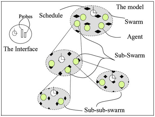
Figure 1. The Swarm's nested inherent hierarchical structure

JADE and FIPA

2.4

JADE (Java Agent DEvelopment Framework, http://sharon.cselt.it/projects/jade/) is a physical multi-agent development framework which complies with FIPA specifications and aims at simplifying the implementation of multi-agent systems. It includes two main products: a FIPA-compliant agent platform and a package to develop Java agents. The advantages of utilizing JADE as a physical agent platform include its capabilities to distribute agents across different operating platforms and to make these agents easily communicate with each other through the Internet. Besides, it can simply integrate with existing systems or databases, and provide graphical interfaces for users to manage their agents.

2.5

FIPA was formed to produce software standards for heterogeneous agent-based systems. Many publicly available implementations of agent platforms conform to FIPA specifications, such as FIPA-OS, JADE, et cetera. Figure 2 illustrates the building layers of physical agents complying with FIPA standards (http://www.fipa.org). FIPA application specifications are example application areas to which FIPA agents can be deployed. They represent ontology and service specifications for a particular domain. FIPA abstract architecture specifications describe the abstract entities that are required to build agent services and environments. FIPA agent communication specifications define Agent Communication Language (ACL) messages, message exchange interaction protocols, communicative acts based on speech act theory and content language representations. FIPA agent management specifications define the control and management of agents within and across agent platforms. FIPA agent message transport specifications define the transport and representation of messages across different network transport protocols, including wire and wireless environments.

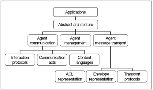
Figure 2. FIPA Specification

The integrated framework

2.6

The integrated agent system, called SPA by extracting initials of the Simulated and Physical Agents, utilizes the corresponding abilities of simulated and physical agents to connect information systems to execute business processes. Figure 3 shows the SPA embedded in an organizational information system to coordinate simulated and physical agents.

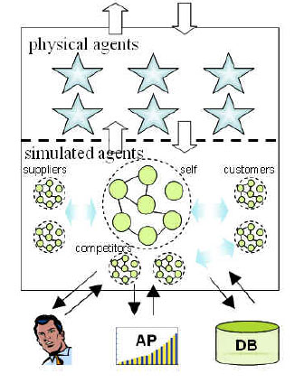
Figure 3. The SPA embedded with information systems

2.7

Simulated agents in the SPA are used to model real world business processes. Agents here may represent an organization's functional entities, such as order management, scheduling production, etc. These simulated agents may receive information from organization's information systems and exchange with partner companies via physical agents. These simulated agents can make use of these information sources to simulate and analyze business processes between these participating organizations. Alternatives suggested by simulation results will pass to corresponding physical agents to make decisions.

2.8

Physical agents gifted with the communication ability can follow decisions suggested by simulated agents to interact with other physical agents embedded in organizational information systems. Figure 4 illustrates the SPA deployed into a certain inter-organizational structure.

Belief system and decision makings

2.9

An agent's belief is its perception of the outside world. The belief of an agent has a deep influence on its decision making. The belief system of an organization maintains its view on the status of the business environment including business-related organizations. The belief system gathers information via physical agents, where information includes inquiries and orders from customers and quotations and deliveries from suppliers. The belief system helps simulated agent analyze gathered information. An organization can make decisions accordingly in the immediate context and then take actions.

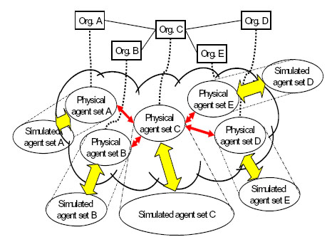
Figure 4. The deployment of the SPA to an inter-organizational structure

The Implementation of the SPA

3.1

The SPA combines simulated and physical agents. Physical agents are established on JADE agent platform to support interactions between organizations. The ontology-based agent communication protocol is defined to facilitate agent communication. Figure 5 portrays the ontology containing eight concepts for physical agents to interact with each other.

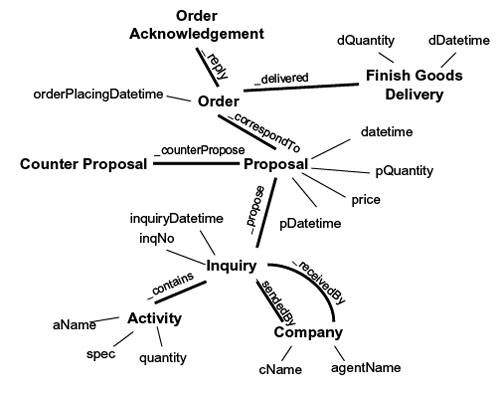
Figure 5. Predefined ontology for physical agents' interaction

Modeling supply chain using object oriented Petri nets (OOPN)

3.2

After modeling functions of simulated and physical agents as shown in Figure 3, the next task is to model the private business processes of individual organizations and their interactions between organizations. In a supply chain with loosely coupled companies, this study uses the object oriented Petri nets (OOPN) to model business processes (Keen & Lakos 1993;Zha 2000;Aalst 2000).

3.3

Petri nets were originally proposed by C. A. Petri in 1962. A Petri net is a graphical and mathematical modeling tool. It consists of places, transitions, tokens, and directed linkages that connect places and transitions. Figure 6 shows a simple graphical model of a Petri net. In a Petri net model, the hollow circle is called a place, which represents a specific resource. The smaller solid circle inside the hollow circle is called a token, which represents the conditions of the resource. The bar, which represents the activity or event of the model, is called a transition. The distribution of tokens among all the places represents the real time resource conditions of the modeled Petri net. The directed linkage represents the input/output relationship between a place and a transition. Transitions are triggered by pre-defined logic rules and the quantity of tokens in the input places. If a transition is triggered, tokens from its prior places will flow to its subsequent places. The number of tokens inside the places keeps updating until no transitions are triggered. If a transition in a Petri net represents such manufacturing activities as machining or assembly, the attributes of this transition must be further defined. The assembling rate and parts consumption rate of an assembly activity should be given before traversing the Petri net.

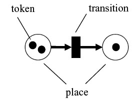
Figure 6. A simple graphical Petri net

3.4

Figure 7(a) demonstrates an example of OOPN. In Figure 7(a), the rectangle with rounded edge illustrates the boundary of an organization. All hollow circles located inside the rectangle represent the resources owned by the organization. The solid, dash, and dotted bars respectively stand for in-house, purchasing, and outsourcing activities of the organization. Each organization can interact with other organizations through activities which compose supply chain processes. Figure 7(b) is the symbolized Petri net corresponding to Figure 7(a). In Figure 7(b), resources and activities are all replaced by symbols. For example, P₄ represents the inventory of standard components and T₂ represents the ordering activity.

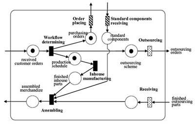
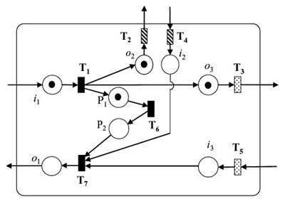
(a) an organization modeled in OOPN	(b) the symbolized model
Figure 7. Modeling the operation of an assembly plant by using OOPN

Generalizing the mathematical expression of OOPN

The OOPN can be easily formulated and coded into computer programs. The generalized mathematical expression of OOPN is formulated as follows:

OOPN=(P, T, F, I, O, P0)

(3.1)

where

P ={P1, P2, …, Pn}

(3.2)

T ={T1, T2, …, Tn}

(3.3)

F ⊆ ( P × T) ∪ ( T × P)

(3.4)

P is a set of places and T is a set of transitions. F is a set of directed linkages that link transitions and places. I is a set of input places which receive tokens from transitions of outside organizations. O is a set of output places which deliver tokens to transitions of outside organizations. P ₀ is the initial marking (condition) of all places.

Supply Chain Example in Electronic Assembly Industry

4.1

This section introduces an example OEM assembly plant, which produces digital still cameras in the electronic industry, to demonstrate how the proposed SPA improves the entire supply chain performance. A digital still camera is a consumer electronic product which has such characteristics of short life cycle, severe competition, high market variation, and quick price falling. Figure 8 shows the BOM (bill of material) of a digital camera, where key components are printed in bold face.

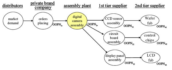
Figure 8. BOM (bill of material) of a digital camera

4.2

Figure 9 shows the most critical portion of a digital camera supply chain. Companies at each tier of a supply chain, ranging from distributors to the second tier suppliers, predict their downstream demand in the coming time periods and places orders to their upstream suppliers. The upstream suppliers deliver their finished goods to their downstream customers. In Figure 9, when the OEM assembly plant receives an order from its customer company, a private brand company, it decides on its outsourcing scheme. The outsourcing scheme needs to determine what materials to purchase, what quantity should be ordered, what manufacturing activities are needed, how activities sequentially are linked or concurrently carried out, and which partners are qualified to be potential suppliers. Once the outsourcing scheme is determined, the OEM assembly plant frequently communicates with its potential suppliers, and negotiates with them to reach a consensus in price and schedule to finish the outsourcing activities. If consensus is reached, the OEM assembly plant sends corresponding orders to suppliers. After all outsourcing activities are carried out and finished components are shipped back, the assembly plant assembles, tests, and packs cameras, and then delivers them to private brand companies. The assembled cameras thereafter are shipped to the distributors.

Figure 9. The critical portion of supply chain of digital camera

Applying OOPN to model the entire supply chain

4.3

Figure 10 shows the Petri net of the entire supply chain corresponding to the supply chain shown in Figure 9. A rounded edge rectangle represents a company. Since the purchasing and manufacturing activities of standard parts are not critical for the digital camera assembly process, they are disabled and rendered in gray color. The mathematic model of the critical portion of a supply chain can then be expressed as follows:

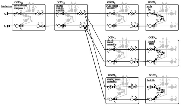
PN = {OOPN11, OOPN21, OOPN31, OOPN32, OOPN33, OOPN41, OOPN42, OOPN43}

(4.1)

OOPNjk=( Pjk, T jk, Fjk, ijk, ojk, P jk0)

(4.2)

4.4

An OOPN in the PN represents the internal workflow of an organization, where j is the j^th tier of the supply chain and k the k^th parallel activity in the j^th tier. For example, OOPN₂₁ represents the assembly plant and OOPN₃₃ represents the display panel assembly.

Figure 10. The Petri net of the entire supply chain

Profiling organizations

4.5

Since the proposed SPA is designed to build distributed supply chains, companies are profiled individually. A file with XML format is used to profile individual organizations. This XML file describes the owner's basic data, such as organization's name, physical agent's id, products or services provided, potential processes to fulfill an received order, suppliers' data, customers' data, etc. Figure 11 shows the XML script that describes the assembly plant in Figure 10. Once the SPA is initialized, the XML file will first be parsed and the organization will then be ready to perform its operations. Other organizations, such as distributors, private brand company, CCD sensor assembly, and LCD fab, can be profiled likewise.

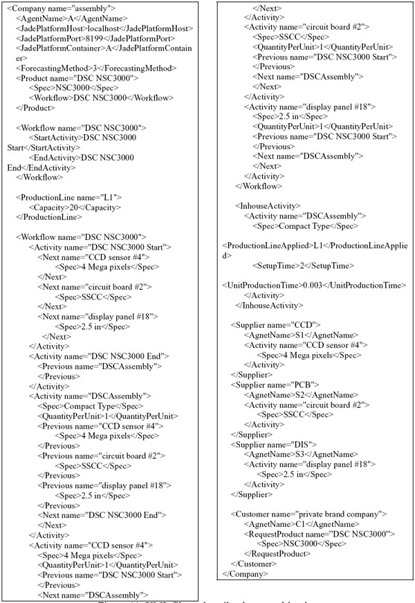
Figure 11. XML file to describe the assembly plant

Modeling time in supply chain environment

4.6

Time in the supply chain example is divided into discrete time periods. A time period, denoted as t, t = 1, 2, 3,…, ∞, is composed of N equally split time slots. N is an any specified integer value, N {1,2,3,..., ∞}. The n^th time slot in time period t is denoted as t_n . For example, 2₃ represents the 3^rd time slot in time period 2. A time period here is analog to a single day, a week, a season or even a business cycle in the real business environment. The length of a time period and the number of time slots in a time period for every company is not necessary to be identical since organizations in a supply chain are distributed. In this study, in order to simplify the settings, all companies use the same length of a time period and the same number of time slots.

Simulating the market demand with unknown patterns

4.7

In order to simulate the situation where some customer demand patterns behind the market are unknown, the market demands are simulated as follows:

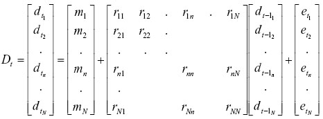
(4.3)

Where

(4.4)

(4.5)

(4.6)

(4.7)

(4.8)

4.8

Equations (4.3) to (4.8) define an auto-regression (AR) model in a matrix format. Vectors D_t and D_t-1 in equations (4.4) and (4.7) represent the market demands in time periods t and t-1, respectively. The component d_tnof D_t is the demand generated during the time slot n in time period t. Vector μ in equation (4.5) is the average demand of the market, where m_n is the average demand at time slot n. Matrix ρ in equation (4.6) is the correlation coefficient between D_t and D_t-1. Vector ρ_n of ρ is the correlation coefficient vector of d_tn and the latest demand D_t-1. The symbol r_np represents the correlation between d_t-1pand d_tn. In equations (4.8), vector ε_t is the error term of AR model. Every ε _tn in ε_t is ε _tn ~ i.i.d., N(0, σ _n ²).

4.9

From the above equations, three additional relations can be further derived as shown in equations (4.9) to (4.11). In equation (4.10), d_t is the total market demand in time period t and d_tn is the market demand during time slot n of time period t.

(4.9)

(4.10)

(4.11)

4.10

In the next section, three different forecasting methods will be tested in five experiments under different market demand settings. In each experiment, every forecasting method is tested with the same simulated market demand in order to compare their experimental results. Therefore, the simulated market demand will be generated beforehand and fed orderly to the distributors T₀₀ of each experiment as time advances. Once the distributors receive the market demand, the entire supply chain is activated.

Modeling OOPN mathematically

4.11

The generalized equations (3.1) to (3.4) can then be applied to the example: With 1≤ j ≤ 3, we obtain OOPN as

Tjk={Tjk1, Tjk3, Tjk5, Tjk7}

(4.12)

ijk={ijk1, ijk3}

(4.13)

ojk={ojk1, ojk3}

(4.14)

Fjk={(ijk1, Tjk1), (Tjk1, ojk3), (ojk3, Tjk3), (Tjk5, ijk3), (ijk3, Tjk7), (Tjk7, ojk1)}

(4.15)

Tjk7 = f (ijk3, t jk7setup, t jk7unit)

(4.16)

Ljk = Ljk7 = t jk7setup + ijk3 * t jk7unit

(4.17)

and with j = 4, we obtain OOPN as

T4k={T4k1, T4k6, T4k7}

(4.18)

P4k={P4k1, P4k2}

(4.19)

F4k={(i4k1, T4k1), (T4k1, P4k1), (P4k1, T4k6), (T4k6, P4k2), (P4k2, T4k7), (T4k7, o4k1)}

(4.20)

T4kl = f (i4kl, t 4klsetup, t 4klunit)

(4.21)

L4kl = t 4klsetup + i4kl * t 4klunit

(4.22)

L4k = L4k6 + L4k7

(4.23)

4.12

Subscript jk denotes the k^th activity of the j^th tier. T_jk1 serves as the sales department of a company, which receives customers' order by a physical agent of the SPA. T_jk3 serves as the procurement department of a company, which forecasts its customers' future demand and determines the outsourcing scheme. T_jk7 is an assembling activity, which is a function of i_jk3, the input quantity, t _jkl^setup, the setup time of transition l, and t _jkl^unit, the unit assembling time of transition l. L_jk is the lead time of T_jk. All transportation time are neglected.

4.13

The directed linkages between companies can be expressed as

F11,21={(T113, i211), (o211, T115)}, F21,31={(T213, i311), (o311, T215)}, F21,32={(T213, i321), (o321, T215)}, F21,33={(T213, i331), (o331, T215)}, F31,41={(T313, i411), (o411, T315)}, F32,42={(T323, i421), (o421, T325)}, F33,43={(T333, i431), (o431, T335)}

(4.24)

4.14

The aforementioned symbol F_11,21 describes the relation between the first activity of the first stage and the first activity of the second stage. In other words, F_11,21 describes the relation between distributors and private brand company.

Forecasting customer demand

4.15

The aim to more precisely forecast customer demand can be reached by discovering the dynamically changing pattern of the market demand. If the dynamic demand pattern is captured, the variation of customer demand will thus be predictable.

4.16

The belief system, data clustering technique and moving average approach are employed in this study to forecast customer future demand. The belief system serves as a data store not only to memorize every received order, but also to update its own customers' demand patterns and then to help simulated agents forecast customers' future demands accordingly. The data clustering technique is employed at the end of every time period to figure out the dynamics of customer demands from the memorized time series data of received orders. The moving average approach is applied at the end of every clustered time slot to predict customer demands.

4.17

Data clustering is a technique to partition data into homogeneous groups in which within-group similarities and between-group dissimilarities are simultaneously maximized. Data are classified into static and dynamic data depending on whether they are time-variant or not. There are five categories of clustering techniques aimed at handling static data, including partitioning, hierarchical, density-based, grid-based, and model-based methods (Han and Kamber 2001).

4.18

Unlike static data, time series data vary dynamically as time advances, and the latest few data generally implicitly imply the moving trend of customer demands. Therefore, the more recent the data is, the more important it is, and the clustering of time series data should be executed frequently to capture the moving trends.

4.19

Time series data in this study are composed of numerous data sequences. A data sequence represents the variation of continually received order quantity in one time period. Each data sequence contains a vector of data items. An entry of a vector represents the received order quantity in a time slot. For example, a vector <10, 11, 13, 13, 4, 3> denotes that this time period contains six time slots, and 10, 11, 13, 13, 4 and 3 units of goods are ordered respectively in these six time slots of this time period.

4.20

Before clustering time series data, data sequences defined in the above paragraph, must be processed to generate initial data clusters first. Entries from different data sequences at the same time slot can be grouped into a data cluster. For example, three data sequences represented as three vectors <13, 11, 10, 10, 5, 3>, <13, 11, 10, 10, 5, 3>, <10, 11, 13, 13, 4, 3> can be clustered into six data clusters; that is, (13, 13, 10), (11, 11, 11), (10, 10, 13), (10, 10, 13), (5, 5, 4) and (3, 3, 3).

4.21

Based on the initially generated clusters, a hierarchical clustering technique, modified from AGNES (AGglomerative NESting) (Kaufmann and Rousseeuw 1990), is applied to merge data clusters in a bottom-up process. The optimum criterion adopted here is to reduce the total sum of the with-in group variances of all the data clusters as much as possible.

4.22

AGNES was first introduced by Kaufmann and Rousseeuw (1990). AGNES is an agglomerative hierarchical clustering method. This method begins by pre-grouping each data item into one cluster, and then merges these clusters into larger clusters iteratively, until all clusters are grouped into one cluster or the termination condition is reached. The modified AGNES algorithm, as presented in Figure 12, is employed to demonstrate the hierarchical clustering process as shown in Figure 13.

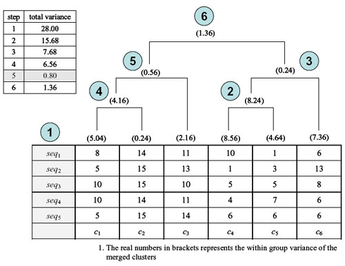
Figure 12. The modified AGNES clustering algorithm

Figure 13a. An example of a complete hierarchical clustering tree

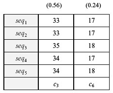
Figure 13b. The optimal clustering results

4.23

Figure 13 shows an example that holds five data sequences and each data sequence contains six data items indicating the quantity of ordered products. According to the modified AGNES algorithm, the optimal clustering policy is to stop merging clusters after step 5 where the sum of within cluster variances does not decrease further. It means that the optimal clustering policy is to merge data items 1,2 and 3 into one cluster, which is (33, 33, 35, 34, 34) and items 4, 5 and 6 into another cluster, (17, 17, 18, 17, 18). The data clusters therefore imply that the sum of ordered items ranges from 33 to 35 from time slot 1 to 3, and the sum of them is 17 or 18 during time slots 4 and 5.

4.24

After the data clustering is executed and the optimal clustering policy is recognized, the next step is to forecast customers' future demand based on the captured pattern. The most intuitive forecast technique is to use the moving average approach (Chen et al. 2000a). Since the lead time depends on every order quantity in this supply chain case, the mathematical expression of moving average is slightly modified as shown from equation (4.25) to (4.30).

4.25

The order up to level y_jk,t,n, lead time L_jk,t for estimate of customer demand _jk,t,c, and order quantity q_jk,t,n at the end time of clustered time slot c in time period t are defined as follows.

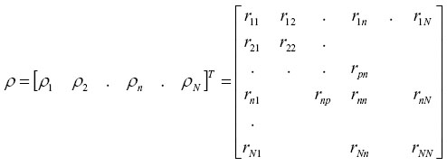
(4.25)

(4.26)

(4.27)

4.26

In equation (4.25), _jk,t,c is the estimate of customer demand forecasted by the k^th activity in the j^th tier at the end of clustered time slot c in time period t. The symbol z_jk for activities of each level is a constant. In (4.26), L_jk,t,c is the estimated lead time corresponding to _jk,t,c. The lead time is estimated by ts_jk the setup time of an activity, tu_jk the time required for each unit product to be manufactured, and Ca_jk the capacity of an organization in a time period. In (4.27), D_jk,t-1,c is the received customer demand at the end time of clustered time slot c in time period t-1 and q_jk,t,n will never be negative. Namely, if q_jk,t,n is less than 0, q_jk,t,n will be 0.

(4.28)

(4.29)

(4.30)

4.27

The symbol w in equations (4.28) and (4.30) is the sliding window size of the moving average. The error of estimate e_jk,t,c of every activity at the end of clustered time slot c in time period t is expressed in equation (4.29). In equation (4.30), σ_ejk,t,c is the standard variance of estimate and C_L,ρ is a constant function of L and ρ (Chen et al. 2000a).

Simulating OOPN modeled supply chains

4.28

An OOPN modeled supply chain, shown in Figure 10, is triggered by distributors' market demands. The market demand in this study is simulated by AR model described in Section 4. The market demand, generated during every time slot, will be delivered to the distributors at the end of every time slot, which is like tokens that flow in the distributors' places.

4.29

A distributor, once receiving the order, stores the order information in its belief system, which is like a place in which tokens are accumulated. Its simulated agents forecast the customer demand at the end of clustered time slots according to the demand information that the belief system has captured. Its physical agent therefore will deliver the forecasted demand to its upstream company, the private brand company. The private brand company and its upstream companies will respond to the demand accordingly. Besides, once reaching the end of a time period, the simulated agent will employ the modified AGNES to update its own customers' demand patterns.

Experimental design

5.1

The goal of designing the experiments is to show the noticeable properties of the SPA proposed in Section 2. In this study, the forecasted error of customer demand is used as a metric to demonstrate and evaluate how much SPA affects the supply chain performance under different experimental settings.

5.2

This study compares three forecasting methods, called simple, moving average, and cluster forecasting methods, respectively, as shown in Figure 14. A company using a simple forecasting method predicts its customer demands according to its total received customer demands during the latest time period, and then forwards the forecasted demands to its upstream suppliers at the end of each time period. The moving average forecasting method takes advantage of the simulated agents' memory to forecast customer demands by using the moving average method with a specified sliding window size, and then forwards the forecasted demands to its upstream suppliers at the end of each time period. The cluster forecasting method utilizes the competences possessed by the SPA that the simulated and physical agents follow the procedure described in Section 4. First, the simulated agent, at the end of each time period, processes the information gathered by physical agents, and employs the modified AGNES clustering technique with the same sliding window size as that in moving average forecasting to identify the dynamics of customers' demand patterns. Second, the simulated agent, at the end of each cluster of time slots, applies the moving average approach to forecasting customers' demands. Finally, the physical agent forwards these orders to its suppliers guided by simulated agents.

5.3

This study set up five experimental settings as shown from Table 1 to 5. In each experimental setting, these three forecasting methods were executed ten rounds according to the defined distribution of market demands. The details of these five experiments are summarized as follows.

5.4

The experimental results of Experiment 1 serve as the basis to compare those from the other four experiments. Experiment 2 replaces the error variance σ² in Experiment 1 with a smaller one, e.g., from 70 to 40, as shown in Table 2. Experiment 3 was conducted under the same settings with Experiment 1 except that the correlation coefficient matrix was changed from 0.45 to 0.80, which indicates that the market demand between t-1 and t of Experiment 3 are more closely related than that of Experiment 1. Experiment 4 tests the performances when the window size of moving average and cluster forecasting methods is 10 (e.g., Table 4). This experiment demonstrates the effect of enlarging the sliding window size on the results by using moving average and cluster forecasting methods. Experiment 5 replaces the parameters ρ,__μ and σ² of Experiment 1 by a complicated matrix and vectors as shown in Table 5.

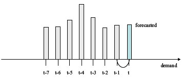
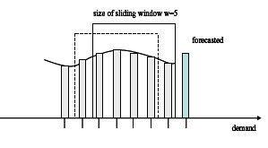
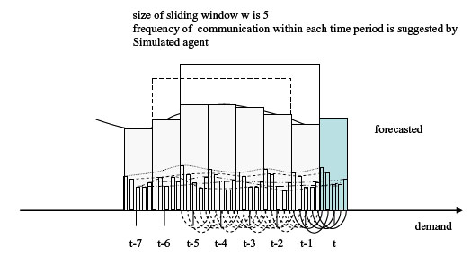
(a) Simple forecasting

(b) Moving average forecasting

(c) Cluster forecasting

Figure 14. Three tested methods

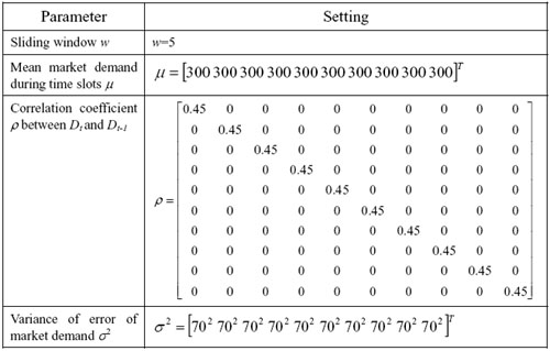
Table 1. The settings of Experiment 1

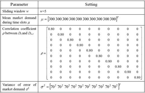
Table 2. The settings of Experiment 2

Table 3. The settings of Experiment 3

Table 4. The settings of Experiment 4

Table 5. The settings of Experiment 5

5.5

Table 6 lists the normalized made-up setup time and unit production/ assembly time of every activity of the order fulfillment process in the supply chain. The capacity Ca_jk of each organization is defined in Table 7.

5.6

In these five experiments, the number of time periods during each experimental round was set to 400, and the number of time slots N in each time period was set to 10. The number of tokens inside places of each OOPN was initialized to 0. The results of all experiments were collected for further analysis in the time period ranging from 100 to 399. Besides, the constant z_jk in equation (4.25) was set to 1.0 and the constant function C_L,ρ in equation (4.30) was set to 2.0 for all activities.

Table 6: Normalized made-up parameter values of activities in the supply chain
Transition	Setup time (tsjk)	Unit production / assembly time (tujk)
T117	3	0
T217	2	0.003
T317	0	0.002
T327	0	0.001
T337	0	0.004
T416	0	0.002
T426	0	0.001
T436	0	0.003
T417	0	0
T427	0	0
T437	0	0

Table 7: Capacities Ca jk of every OOPN jk set up in the supply chain
Transition	Capacity
OOPN11	10
OOPN21	10
OOPN31	10
OOPN32	5
OOPN33	5
OOPN41	10
OOPN42	5
OOPN43	5

Experimental Results and Discussions

6.1

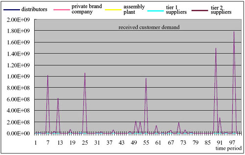
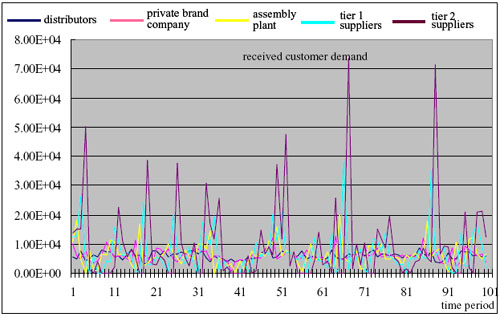
(a) Bullwhip effect

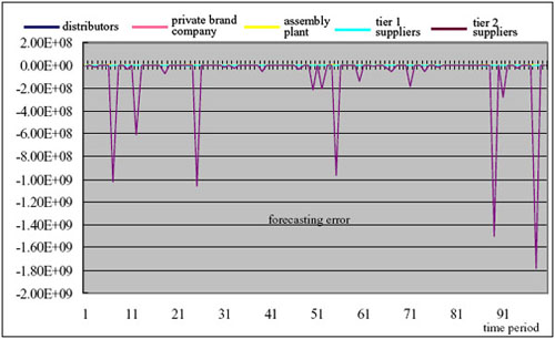
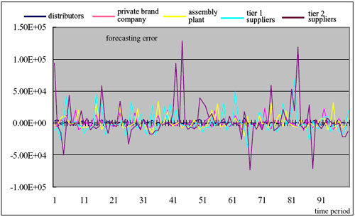
(b) Forecasting errors

Figure 15. Results of the simple forecasting in Experiment 2

(a) Bullwhip effect

(b) Forecasting errors

Figure 16. Results of the moving average forecasting in Experiment 2

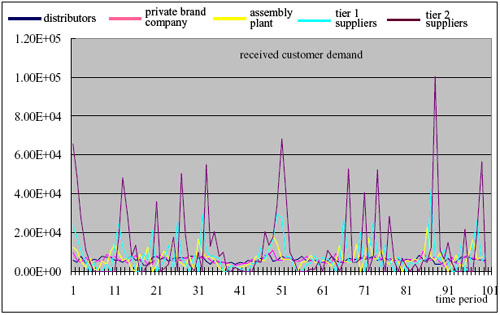
(a) Bullwhip effect

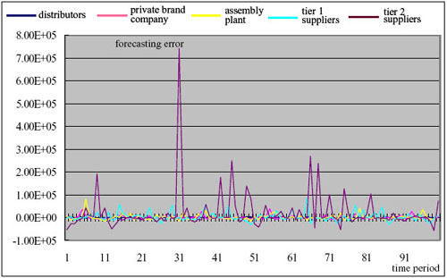
(b) Forecasting errors

Figure 17. Results of the cluster forecasting in Experiment 2

6.2

Table 8 to 12 shows the comparisons between the reduction of forecasting errors from moving average to simple forecasting and that from cluster to moving average forecasting. Tables 8 to 12 first show the significance tests of the reduction of forecasting errors in absolute values and then in the percentage of significance by t-test (α ≤ 0.05).

6.3

The results of Experiment 1 indicate that the moving average forecasting significantly reduced the forecasting errors of all five tiers comparing those that the simple forecasting did. Besides, the reduction of forecasting errors made by cluster forecasting is significantly less in tiers 2, 3, 4, and 5 than those made by the moving average forecasting as shown in Table 8.

6.4

In Experiment 2, moving average and cluster forecasting methods significantly outperform simple forecasting. Besides, the results of Experiment 2 show that cluster forecasting contributes less toward reducing the forecasting errors than moving average forecasting in the first three tiers of this supply chain when the variation of market demand is small as seen in Table 9. In Table 10, the results of Experiment 3 show that cluster forecasting outperformed moving average forecasting in the 4^th and 5^th tiers of this supply chain when the demand pattern between time periods t and t-1 was similar. However, in the first and third tiers, the moving average forecasting outperformed the cluster forecasting.

6.5

Table 11 shows that the moving average forecasting outperformed the cluster forecasting in Experiment 4 where the supply chain demands were forecasted by large sliding window sizes. Nevertheless, in the 4th and 5th tiers, the cluster forecasting still outperformed the moving average forecasting. The results of Experiment 5 shown in Table 12 infer that cluster forecasting significantly reduces the forecasting errors than moving average forecasting did in tiers 2, 3, 4, and 5 of the supply chain example when the implicit pattern of market demand is complicated.

6.6

To sum up, the moving average and the cluster forecasting methods outperform the simple forecasting under various experimental settings. The cluster forecasting, taking advantages of the integrated agents system, i.e., SPA, to employ the belief system, the modified AGNES clustering, and the moving average approaches, outperforms the moving average forecasting at handling uncertain business environments. Especially, for those upstream suppliers who suffer from the severe bullwhip effect, cluster forecasting effectively helps tame the bullwhip effect and reduce the forecasting errors.

6.7

The complete source code of this study is opened at http://mx.nthu.edu.tw/~frlin/SPA. Following the install instructions, readers can build the supply chain environment and give alternative parameter values to execute different experiments and test the performance improvement of SPA.

Table 8: Significance test of the decrease of forecasting errors by t-test (Experiment 1)
Exp#	Method comparison	Stage 1. distributors	Stage 2. private brand company	Stage 3. assembly plant	Stage 4. tier 1 suppliers	Stage 5. tier 2 suppliers
1	moving average vs. simple	6.27*	4.18*	4.88*	6.37*	9.58*
	cluster vs. moving average	-1.04	2.64*	1.88*	4.59*	5.95*
2	moving average vs. simple	7.15*	3.25*	5.61*	6.80*	9.47*
	cluster vs. moving average	-0.85	2.53*	3.44*	4.62*	5.01*
3	moving average vs. simple	5.64*	2.44*	5.01*	6.58*	8.68*
	cluster vs. moving average	-0.76	1.71*	3.96*	3.78*	4.07*
4	moving average vs. simple	6.43*	3.33*	4.80*	6.18*	10.29*
	cluster vs. moving average	-1.20	2.89*	3.74*	2.91*	4.40*
5	moving average vs. simple	6.28*	3.39*	4.80*	6.82*	10.24*
	cluster vs. moving average	-1.00	0.71	3.14*	2.50*	3.95*
6	moving average vs. simple	7.27*	3.04*	4.73*	6.23*	10.08*
	cluster vs. moving average	-1.31	1.05*	3.06*	2.36*	3.09*
7	moving average vs. simple	6.83*	2.65*	5.92*	6.62*	10.43*
	cluster vs. moving average	-1.35	1.02	0.86	4.04*	3.70*
8	moving average vs. simple	7.13*	3.23*	5.53*	6.96*	9.50*
	cluster vs. moving average	-0.90	1.99*	2.90*	3.40*	3.32*
9	moving average vs. simple	8.01*	2.19*	5.43*	6.71*	9.18*
	cluster vs. moving average	-1.25	2.97*	3.41*	2.58*	5.40*
10	moving average vs. simple	6.16*	3.61*	4.34*	6.55*	9.53*
	cluster vs. moving average	-1.34	1.93*	3.49*	2.03*	3.31*
% of significance	moving average vs. simple	100%	100%	100%	100%	100%
	cluster vs. moving average	0%	80%	90%	100%	100%

*significant, α≤ 0.05, n1=300, n2=300, t=1.64

Table 9: Significance test of the decrease of forecasting errors by t-test (Experiment 2)
Exp#	Method comparison	Stage 1. distributors	Stage 2. private brand company	Stage 3. assembly plant	Stage 4. tier 1 suppliers	Stage 5. tier 2 suppliers
1	moving average vs. simple	6.96*	6.24*	6.75*	5.27*	3.96*
	cluster vs. moving average	-1.69	0.12	2.28*	2.99*	5.21*
2	moving average vs. simple	8.04*	7.66*	6.91*	7.36*	3.74*
	cluster vs. moving average	-1.52	-0.01	2.01*	3.15*	4.69*
3	moving average vs. simple	7.25*	6.69*	6.45*	5.44*	3.90*
	cluster vs. moving average	-2.16	0.79	2.15*	3.49*	5.16*
4	moving average vs. simple	7.16*	6.47*	6.17*	6.39*	4.73*
	cluster vs. moving average	-1.73	0.27	1.39	3.17*	4.33*
5	moving average vs. simple	7.87*	6.71*	6.18*	6.56*	4.68*
	cluster vs. moving average	-2.68	-0.15	2.38*	2.57*	4.69*
6	moving average vs. simple	7.51*	6.75*	5.82*	5.52*	4.32*
	cluster vs. moving average	-1.96	1.21	2.37*	3.48*	4.72*
7	moving average vs. simple	8.35*	6.56*	7.13*	6.42*	4.45*
	cluster vs. moving average	-2.88	-0.58	0.85	2.32*	4.27*
8	moving average vs. simple	7.60*	6.75*	6.40*	6.51*	4.38*
	cluster vs. moving average	-2.23	-0.75	1.08	2.15*	3.67*
9	moving average vs. simple	7.67*	6.79*	6.03*	6.25*	4.14*
	cluster vs. moving average	-1.69	0.19	1.35	2.98*	4.40*
10	moving average vs. simple	6.58*	6.16*	6.40*	2.91*	4.65*
	cluster vs. moving average	-1.99	-1.32	1.25	2.52*	4.19*
% of significance	moving average vs. simple	100%	100%	100%	100%	100%
	cluster vs. moving average	0%	0%	50%	100%	100%

*significant, α≤0.05, n1=300, n2=300, t=1.64

Table 10: Significance test of the decrease of forecasting errors by t-test (Experiment 3)
Exp#	Method comparison	Stage 1. distributors	Stage 2. private brand company	Stage 3. assembly plant	Stage 4. tier 1 suppliers	Stage 5. tier 2 suppliers
1	moving average vs. simple	6.83*	0.31	6.79*	8.14*	5.53*
	cluster vs. moving average	-2.36	0.24	-2.11	3.25*	3.92*
2	moving average vs. simple	6.22*	1.19	6.17*	7.64*	5.83*
	cluster vs. moving average	-3.23	0.82	-1.74	3.30*	3.98*
3	moving average vs. simple	6.50*	-0.56	6.61*	8.02*	6.25*
	cluster vs. moving average	-2.25	0.84	-0.04	3.58*	4.11*
4	moving average vs. simple	5.52*	1.07*	6.28*	7.54*	4.55*
	cluster vs. moving average	-2.91	0.31	-0.90	4.48*	4.82*
5	moving average vs. simple	5.79*	-0.61	6.70*	7.97*	4.24*
	cluster vs. moving average	-2.01	1.07	-0.57	3.63*	5.21*
6	moving average vs. simple	6.90*	0.20	7.64*	8.50*	2.96*
	cluster vs. moving average	-2.05	2.09*	-1.39	4.64*	5.53*
7	moving average vs. simple	6.51*	-1.68	6.91*	8.85*	3.79*
	cluster vs. moving average	-3.18	-0.27	-0.35	3.12*	5.03*
8	moving average vs. simple	6.39*	0.03	5.94*	7.86*	3.54*
	cluster vs. moving average	-2.30	2.31*	-1.65	4.22*	6.03*
9	moving average vs. simple	6.13*	1.75*	5.59*	7.33*	6.22*
	cluster vs. moving average	-2.38	0.54	1.30	3.32*	4.37*
10	moving average vs. simple	7.31*	-0.37	6.73*	7.98*	5.68*
	cluster vs. moving average	-2.65	0.79	-1.88	3.39*	4.58*
% of significance	moving average vs. simple	100%	20%	100%	100%	100%
	cluster vs. moving average	0%	20%	0%	100%	100%

*significant, α≤0.05, n1=300, n2=300, t=1.64

Table 11: Significance test of the decrease of forecasting errors by t-test (Experiment 4)
Exp#	Method comparison	Stage 1. distributors	Stage 2. private brand company	Stage 3. assembly plant	Stage 4. tier 1 suppliers	Stage 5. tier 2 suppliers
1	moving average vs. simple	9.25*	4.68*	7.48*	6.95*	9.32*
	cluster vs. moving average	-0.77	0.53	1.96*	2.21*	2.01*
2	moving average vs. simple	8.12*	4.61*	6.27*	6.67*	9.14*
	cluster vs. moving average	-1.05	0.96	1.32	0.05	0.99
3	moving average vs. simple	8.62*	4.69*	7.04*	6.26*	10.03*
	cluster vs. moving average	-0.97	0.73	1.67*	1.92*	3.13*
4	moving average vs. simple	6.84*	5.26*	5.97*	6.31*	9.38*
	cluster vs. moving average	-0.63	0.32	0.83	3.76*	2.79*
5	moving average vs. simple	7.32*	4.20*	6.74*	6.63*	10.14*
	cluster vs. moving average	-1.24	0.47	0.93	0.28	2.73*
6	moving average vs. simple	7.91*	5.05*	6.30*	6.51*	11.48*
	cluster vs. moving average	-0.99	-0.51	1.84*	2.00*	2.70*
7	moving average vs. simple	6.67*	4.65*	6.14*	6.02*	9.29*
	cluster vs. moving average	-0.63	0.41	2.71*	2.34*	3.50*
8	moving average vs. simple	7.48*	5.86*	7.01*	6.25*	9.68*
	cluster vs. moving average	-0.94	0.86	0.88	1.65*	2.22*
9	moving average vs. simple	7.52*	5.02*	6.21*	6.30*	10.20*
	cluster vs. moving average	-1.44	-0.59	1.12	2.51*	1.48
10	moving average vs. simple	6.95*	5.73*	5.42*	6.26*	9.82*
	cluster vs. moving average	-1.15	-1.05	0.51	1.13	2.18*
% of significance	moving average vs. simple	100%	100%	100%	100%	100%
	cluster vs. moving average	0%	0%	40%	70%	80%

*significant, α≤0.05, n1=300, n2=300, t=1.64

Table 12: Significance test of the decrease of forecasting errors by t-test (Experiment 5)
Exp#	Method comparison	Stage 1. distributors	Stage 2. private brand company	Stage 3. assembly plant	Stage 4. tier 1 suppliers	Stage 5. tier 2 suppliers
1	moving average vs. simple	6.10*	3.78*	4.63*	6.42*	8.76*
	cluster vs. moving average	-0.71	2.78*	3.91*	4.25*	5.21*
2	moving average vs. simple	5.91*	4.33*	3.97*	6.17*	10.40*
	cluster vs. moving average	-1.44	2.31*	3.03*	2.68*	5.20*
3	moving average vs. simple	6.53*	3.46*	4.29*	5.93*	9.72*
	cluster vs. moving average	-0.45	3.07*	4.05*	2.36*	3.15*
4	moving average vs. simple	6.73*	3.83*	4.37*	6.43*	9.17*
	cluster vs. moving average	-1.32	2.21*	4.17*	4.23*	5.55*
5	moving average vs. simple	7.72*	3.46*	5.05*	7.04*	9.59*
	cluster vs. moving average	-1.32	1.80*	3.13*	3.17*	5.68*
6	moving average vs. simple	6.77*	4.43*	4.96*	6.82*	9.84*
	cluster vs. moving average	-0.88	2.38*	3.80*	2.86*	3.76*
7	moving average vs. simple	6.07*	2.81*	5.31*	6.14*	9.72*
	cluster vs. moving average	-1.69	3.29*	2.20*	3.85*	3.85*
8	moving average vs. simple	6.44*	4.27*	5.33*	6.68*	9.33*
	cluster vs. moving average	-0.94	1.33	3.07*	4.01*	5.83*
9	moving average vs. simple	6.92*	5.26*	4.75*	5.99*	8.88*
	cluster vs. moving average	-1.54	1.81*	4.65*	2.08*	2.10*
10	moving average vs. simple	6.19*	3.23*	4.76*	6.64*	10.51*
	cluster vs. moving average	-0.74	3.20*	3.95*	3.27*	3.84*
% of significance	moving average vs. simple	100%	100%	100%	100%	100%
	cluster vs. moving average	0%	90%	100%	100%	100%

*significant, α≤0.05, n1=300, n2=300, t=1.64

Conclusion and Future Research

7.1

The objective of this study is to propose an integrated agents system (SPA) to provide an efficient way for organizations to meet the challenges in managing supply chains. The SPA, which coordinates simulated and physical agents, is able to support real-time online decision makings. This study uses a supply chain that produces digital still cameras as an example to demonstrate how SPA works. The improvement of bullwhip effect is adopted as a metric to show the contributions of SPA to the performance enhancement of the supply chain management.

7.2

In this study, SPA, the integrated agents system, which combines the analysis and decision support capabilities of simulated agents and the communication facilitation from physical agents, helps supply chain companies easily interact with business related partners and furthermore help them make such decisions as placing the accurate order quantity at the appropriate time. As the experimental results shown in Section 6, though the bullwhip effect is inevitable, SPA can effectively reduce the bullwhip effect without breaking the existing business rules. The characteristics of the physical agents in SPA can be portrayed as follows: (1) they meet real world business conditions (organizations are decentralized), and (2) organizations can frequently and easily communicate with others to gather environmental information. The characteristics of simulated agents are specified as follows: (1) they support decision making with incomplete information under uncertain situations, (2) they can update their belief systems by perceiving information from outside world, and (3) learning models can be embedded in simulated agents to model, analyze and forecast business transactions.

7.3

In this study, object-oriented Petri nets, regarding an organization as a service provider, are used to model business processes. An organization can thus easily connect its business partners to form supply chains efficiently. The framework can be extended to work with the Web service platform. The embedded autonomy of agent systems in a Web service inherits the merits of the SPA in efficiency, effectiveness, and flexibility to deliver Web services, such as automated partner selection facilitated by simulated trust and negotiation agents and physical negotiation agents via UDDI and WSDL protocols.

7.4

This study simulated only a simple supply chain to prove that the SPA does help firms enhance their entire supply chain performance. Advanced research efforts may be spent on such directions as migrating the SPA into a service oriented architecture, building different learning and inference models into the belief system of simulated agents, and developing the context-dependent strategies of pricing, transportation and inventory for organizations involved in different supply chain structures.

References

AALST I W, Desel J and Oberweis A (2000) Business process management: models, techniques, and empirical studies. Lecture Notes in Computer Science, 1806, Berlin, Heidelberg, New York, pp. 254-273.

BAGANHA M P and Cohen M A (1998) The stabilizing effect of inventory in supply chains. Operations Research, 46(3), pp. 572-583.

BRUSTOLONI J C (1991) Autonomous agents: characterization and requirements. Carnegie Mellon Technical Report CMU-CS-91-204, Pittsburgh: Carnegie Mellon University.

CARLSSON C & Fuller R (2001) Reducing the bullwhip effect by means of intelligent, soft computing methods. Proceedings of the 34th Hawaii International Conference on System Sciences.

CHANDRA C and Grabis J (2005) Application of multi-steps forecasting for restraining the bullwhip effect and improving inventory performance under autoregressive demand. European Journal of Operational Research, 166(2), pp.337-350.

CHEN F, Drezner Z, Ryan J K and Simch-levi D (2000a) Quantifying the bullwhip effect in a simple supply chain: The impact of forecasting. Management Science, 46(3), pp.436-443.

CHEN F, Drezner Z, Ryan J K and Simchi-levi D (2000b) The impact of exponential smoothing forecasts on the bullwhip effect. Naval Research Logistics, 47, pp.269-286.

DAVIDSSON P (2002) Agent Based Social Simulation: A Computer Science View. Journal of Artificial Societies and Social Simulation, 5(1), https://www.jasss.org/5/1/7.html

DEJONCKHEERE J, Disney S M, Lambrecht M R and Towill D R (2004) The impact of information enrichment on the bullwhip effect in supply chains: A control engineering perspective. European Journal of Operational Research, 153(3), pp. 727-750.

FONER L N (1993) What's an agent, anyway? A sociological case study. Agents Memo 93-01. Agents Group. Cambridge, MA: MIT Media Lab.

FORRESTER J W (1958) Industrial dynamics: A major breakthrough for decision makers. Harvard Business Review, 36(4), pp.37-66.

FOX, M S, Barbuceanu M, and Teigen, R (2000) Agent-oriented supply-chain management. International Journal of Flexible Manufacturing Systems, 12(2,3), pp.165-188.

HAN J and Kamber M (2001) Cluster analysis. In Data Mining: Concepts and Techniques, Morgan Kaufmann Publishers, San Francisco, CA, pp. 335-394.

HAYES-ROTH B (1995) An architecture for adaptive intelligent systems. Artificial Intelligence: Special Issue on Agents and Interactivity, 72, pp. 329-365.

HOSODA T and Disney S M (2006) On variance amplification in a three-echelon supply chain with minimum mean square error forecasting. The International Journal of Management Science, 34(4), pp. 344-358.

JIAO J, You X and Kumar A (2006) An agent-based framework for collaborative negotiation in the global manufacturing supply chain network. Robotics and Computer-Integrated Manufacturing, 22(3), pp. 239-255.

KEEN C D and Lakos C A (1993) A methodology for the construction of simulation models using object-oriented petri nets. Proc. of the European Simulation Multi-conference, pp. 267-271.

KAIHARA T (2003) Multi-agent based supply chain modeling with dynamic environment. International Journal of Production Economics, 85(2), pp.263-269.

KAUFMAN L and Rousseeuw P J (1990) Finding Groups in Data: an Introduction to Cluster Analysis, John Wiley & Sons.

KIMBROUGH S O, Wu D J and Fang Z (2002) Computers play the beer game: can artificial agents manage supply chains? Decision Support Systems, 33(3), pp.323-333.

KRAUSE S, Morais de Assis Silva F, Magedanz T, Popescu-Zeletin R, Falsarella O M and Raul Arias Mendez C (1997) MAGNA -- A DPE-based platform for mobile agents in electronic service markets. Proceedings of Third International Symposium on Autonomous Decentralized Systems, pp.93-102.

LEE H L, Padmanabhan P and Whang S (1997a) The paralyzing curse of the bullwhip effect in a supply chain. Sloan Management Review, Spring 1997, pp. 93-102.

LEE H L, Padmanabhan P and Whang S (1997b) Information distortion in a supply chain: the bullwhip effect. Management Science, 43(4), pp. 546-558.

LEE H L, Padmanabhan P and Whang S (2004a) information distortion in a supply chain: The bullwhip effect. Management Science, 50(12), pp.1875-1886.

LEE H L, Padmanabhan P and Whang S (2004b) Comments on 'information distortion in a supply chain: the bullwhip effect' the bullwhip effect: reflections. Management Science, 50(12), pp. 1887-1893.

LIN F R and Lin Y Y (2004) Integrating multi-agent negotiation to resolve constraints in fulfilling supply chain orders. The 8th Pacific-Asia Conference on Information Systems, Shanghai, China.

LIN F R and Shaw M J (1998) Reengineering the order fulfillment process in supply chain networks. International Journal of Flexible Manufacturing Systems, 10(3), pp.197-229.

LUNA F and Stefansson B (2000) Economic Simulation in Swarm: Agent-based Modeling and Object Oriented Programming, Kluwer Academic Publishers, Boston.

MAES P (1995) Artificial life meets entertainment: life like autonomous agents. Communications of the ACM, 38(11), pp. 108-114.

METTERS R (1996) Quantifying the bullwhip effect in supply chains. MSOM Conf. pp. 264-269.

MINAR N, Burkhart R, Langton C and Askenazi M (1996) The swarm simulation system: a toolkit for building multi-agent simulations. http://www.swarm.org.

PETRI C A (1962) Fundamentals of a theory of asynchronous information flow. IFIP Congress.

TERNA P (1998) Simulation tools for social scientists: building aAgent based models with Swarm. Journal of Artificial Societies and Social Simulation, 1(2), https://www.jasss.org/1/2/4.html

THONEMANN U W (2002) Improving supply-chain performance by sharing advance demand information. European Journal of Operational Research, 142(1), pp. 81-107.

STRADER T J, Lin F R and Shaw M J (1998) Simulation of order fulfillment in divergent assembly supply chains. Journal of Artificial Societies and Social Simulation, 1(2), https://www.jasss.org/1/2/5.html

WAGNER T, Guralnik V and Phelps J (2003) TAEMS agents: enabling dynamic distributed supply chain management. Electronic Commerce Research and Applications, 2(2), pp.114-132.

WEIDMANN N B and Girardin L (2005) Technical note: evaluating java development kits for agent-based modeling. Journal of Artificial Societies and Social Simulation, 8(2), https://www.jasss.org/8/2/8.html

WOOLDRIDGE M and Jennings N R (1995) Agent theories, architectures, and languages: a survey. In M. Wooldridge and N.R. Jennings (Eds.), Intelligent Agents, Berlin: Springer-Verlag, pp.1-22.

YUNG S K, Yang C C, Lau A SM and Yen J (2000) Applying multi-agent technology to supply chain management. Journal of Electronic Commerce Research, 1(4), pp.119-132.

ZHA X F (2000) An object-oriented knowledge based Petri net approach to intelligent integration of design and assembly planning. AI in Engineering, 14(1), pp.83-112.

Return to Contents of this issue

© Copyright Journal of Artificial Societies and Social Simulation, [2006]