©Copyright JASSS

JASSS logo ----

Guillaume Deffuant (2006)

Comparing Extremism Propagation Patterns in Continuous Opinion Models

Journal of Artificial Societies and Social Simulation vol. 9, no. 3
<https://www.jasss.org/9/3/8.html>

For information about citing this article, click here

Received: 04-Jan-2006    Accepted: 10-Apr-2006    Published: 30-Jun-2006

PDF version


* Abstract

We compare patterns of extremism propagation yielded by 4 continuous opinion models, when the main parameters vary, on different types of networks (total connection, random network, lattice). In two models the individuals take into account the uncertainty of their interlocutor, and they show similar patterns, with a higher probability of double extreme convergence than in the other couple of models (in which the interlocutor's uncertainty is not taken into account). The addition of noise does not change significantly the results, except that it favours the single extreme convergence in some models. The lattice topology of interactions provides results which are significantly different from the ones obtained with a random network of similar connection density. We identify 3 typical behaviours with a single initial extremist, which help to explain the different results. In particular, we observe that the single extreme convergence is favoured by small shortest paths between all pairs of nodes in the network.

Keywords:
Continuous Opinion, Extremism, Convergence Pattern

* Introduction

1.1
In recent years, we have proposed several models of opinion dynamics and used them to model the influence of individuals with extreme opinion in a population of moderates (Deffuant et al. 2002, Amblard and Deffuant 2004, Weisbuch et al. 2002, Weisbuch et al. 2005). These models rely on several general qualitative hypotheses on the agent behaviour:

1.2
It is implicit in these hypotheses that a distance between opinions can be defined, and that a threshold on this distance determines if the agent will be influenced. The classical binary models in which the opinion is either 0 or 1 (e.g. Galam and Moscovici 1991,Young 1998), are not appropriate to express the richness of these hypotheses, because in these models the opinion distance can only be 0 or 1. Nevertheless, there is a wide variety of possibilities to express mathematically these qualitative hypotheses.

1.3
The simplest is the bounded confidence model (Hegselmann & Krause 2002, Deffuant et al. 2001; Weisbuch et al. 2002). In this model, each agent has a threshold in addition to its opinion (sometimes interpreted as an uncertainty), and it ignores opinions which are at a distance beyond this threshold. In Hegselmann & Krause (2002), an agent takes into account an average influence of all its neighbours, whereas in Deffuant et al. (2001) only pair interactions are simulated. The consequences of this choice are studied in Urbig & Lorenz (2004). More recently, Hegselmann & Krause (2005) studied other variants of averaging within the bounded confidence model. Stauffer et al. (2004) proposed a discrete version of the bounded confidence model and Urbig (2003) a version where agents have a discrete expression of their continuous opinions.

1.4
This model is generalised to a case where agents can have different uncertainties: extremists are initialised with an opinion equal to one of the bounds, and a very low uncertainty, moderates with a randomly chosen opinion and a larger uncertainty. The dynamics on uncertainties can be very similar to the one on opinions, as in Weisbuch et al. (2002).

1.5
It is possible to consider different types of influence dynamics which build on this initial principle. For instance, the Smooth Bounded Confidence model (Deffuant et al. 2004), is another mathematical possibility for expressing the general hypothesis that the influence decreases very rapidly to zero when the distance of opinions is above a threshold. The Relative Agreement (RA) model (Deffuant et al. 2002) expresses the additional hypothesis that an agent takes into account the uncertainty of its interlocutor, and that it will be more influenced if its interlocutor is more certain than itself. Again, other possibilities could have been chosen.

1.6
Edmonds (2006) suggests that the general behaviour of these models is very sensitive to contingent mathematical choices, and to the addition of noise. The objective of this paper is to investigate, on a limited set of chosen models, the sensitivity of the convergence patterns to the modelling choices. However, we consider that the type of noise proposed by Edmonds is in contradiction with the hypotheses of the models. We argue that a noise which is moderated by the uncertainty of the agents respects these hypotheses, and is therefore more appropriate to test the model robustness to noise.

1.7
We limited our investigation to the continuous opinion dynamics models. We chose four of them:

1.8
We perform the same systematic experiment designs on these models, in which we vary the essential parameters, for 3 networks of interactions: total connection, random Erdos-Renyi network with 4 neighbours on average, lattice. We then compare the patterns of types of convergence, considering the 3 types that we identified in previous work (moderate convergence, double extreme convergence, single extreme convergence).

1.9
The paper is organised as follows. We first provide the details on the different models and on the indicators we use to define the types of convergence (which are a bit different from the ones used in previous papers). Then, we present the convergence results from systematic experiment designs where the uncertainty of the moderates and the initial proportion of extremists vary, for a given value of μ, the intensity of interactions. We then propose some results about the important influence of μ (which was already pointed out by Urbig and Lorenz (2004)). This leads us to focus on the difference of convergence patterns that appear between the lattice and random network with the same average connectivity. Understanding this difference leads us to investigate the cases of single initial extremist in the population and to relate this to a closer analysis of the network properties.

* The considered models of continuous opinion influence

Features which are common to all the model variants

2.1
The considered models share the following aspects :

2.2
Moreover, for all the models, when an individual with opinion x and uncertainty u meets another individual of opinion x' and uncertainty u', the modifications of the individuals uncertainties and opinions follow the same type of function. They depend on a kernel function of x, x' and u', which takes u as a parameter. Let ku be this function.

Equation (1)

Equation (2)

In the next paragraph, we list the variants of the models corresponding to different choices for ku.

Variants of the kernel function

Bounded Confidence (BC)

2.3
The initial bounded confidence model including only equations (1), was modified, for instance in Weisbuch et al. (2005), to include equations (2) on the uncertainties. In this case, the kernel function is independent of u', it is of Heaviside type :

Equation (3)

The Gaussian Bounded Confidence (GBC)

2.4
In this case, the kernel function has the form of a Gaussian function, and is also independent of u':

Equation (4)

The relative agreement Model (RA)

2.5
The relative agreement (Deffuant et al. 2002) introduces a new assumption: individuals take into account the uncertainty of their interlocutor, and interlocutors with a low uncertainty (high confidence) tend to be more influential than those with a high uncertainty. The rules use v, the size of the overlap between segments [x-u, x+u] and [x'-u',x'+u'].

Equation (5*)
* The author is grateful to Sascha Holzhauer for having noticed an error in formula (5), which has been corrected in May 2012.

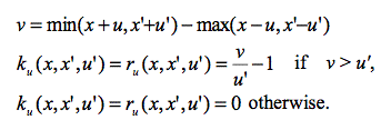
The value of this function is 1 when the segment [x'-u',x'+u'] is totally included in the segment [x-u, x+u]. Otherwise, it is lower than 1.

The Gaussian Bounded Confidence Models with influence of uncertainty (GBCU)

2.6
This model expresses the same assumption as the RA model, considering that low uncertainty gives more influence than high uncertainty. This is expressed as follows:

Equation (5)

With this kernel, if u is much smaller than u', then the change is necessarily small, because then gu(u',0) is small.

Introduction of noise

2.7
As suggested in Edmonds (2006), a good way to test the robustness of the results is to check if the addition of some noise changes the results. However, in Edmonds proposal the same noise is applied to all individuals. Therefore, extremists can suddenly strongly change their opinion. This is in contradiction with the assumption of the model stating that the extremists are very convinced of their opinion. To keep the rationale of the model, we consider that the level of random variations in the opinion is moderated by the level of uncertainty.

2.8
To implement this idea, at each time step, with a probability of 0.1, we add to the opinion of each individual, a random number uniformly distributed between -0.3 and +0.3, multiplied by the uncertainty of this individual. In this case, the opinions can be slightly higher than 1 or lower than -1, but this does not introduce any particular problem.

* Method for designing experiments and expressing the results

Convergence types

3.1
For all the models, we would like to identify the parameter values leading to the 3 convergence types identified on the RA model: moderate, double extreme and single extreme convergence. These convergence types are illustrated on figure 1. The type of convergence depends on the values of the parameters and we aim to compare the patterns of convergence in the parameter space for the different variants of the model.

Figure
Figure 1. The 3 convergence types. N = 50, 2 extremists at +1 and -1, ue = 0.01 (represented in red), μ = 0.3. Top: U = 0.3, RA model. Moderate convergence (X=0.62, n =3.8). Middle: U = 0.9, RA model. Double extreme convergence (X=0.99, n=1.77). Bottom : U = 1.3, GBCU model. Single extreme convergence (X=0.97, n=1.08). See paragraph 3.2 for definitions of X and n

Computing the clusters

3.2
We only consider the clusters of initially moderate agents (i.e. initialised with uncertainty U), because our goal is to evaluate the effect on moderates of different configurations of extremists. To compute the clusters, we define a minimum distance ε between opinions, below which we consider that they belong to the same cluster. We compute the clusters as groups of agents such that between any couple of agents of opinions x and x' in the group, there is a list of agents in the group of opinions (x1, x2, …, xk) making a chain of couples with a distance below ε. More precisely:

Equation (7)

In practice, we chose ε = 0.01.

3.3
The following pseudo-code can be used to compute the clusters. Initially moderate and extremist agents are tagged at the beginning of the simulation. Method addAll() adds all the elements of the argument (supposed to be a list) to the argument (supposed to be a list as well). Method removeAll() removes from the recipient all the elements of the argument (both are supposed to be lists).
epsilon := 0.01;
toDo := indices of initially moderate agents;
clusters := List.new;
while (toDo.size > 0):
	currentCluster := List.with(toDo[1]);
	newAdded := List.with(toDo[1]);
	while(newAdded.size > 0):
		newAdded := List.new;
		for (j := 1, toDo.size)
			if (distance(currentCluster, toDo[j]) < epsilon) newAdded.add(toDo[j]);
		toDo.removeAll(newAdded);
		currentCluster.addAll(newAdded);
 	end while
 	clusters.add(currentCluster);
end while
return(clusters)

Characterisation of the convergence type

3.4
To characterise the convergence type of a simulation, we combine two indicators:

3.5
The generalised number of clusters gives the exact number of clusters when they all include the same proportion of individuals, and intermediate values for intermediate situations. The rationale is that small clusters count less.

3.6
We combine the two indicators to compute the convergence type, with the following rules:

3.7
To decide when to stop a simulation, we computed how the value of X is modified after 500 steps. If the modification is higher than 0.01, then we run 500 more steps. Moreover, if X > 0.9, we know we can stop the experiment.

Pseudo-code running one experiment

3.8
For sake of clarity, we provide the pseudo-code of one experiment. In this code, population is the list of agents, agent.neighbours is the list of indices of agent neighbours, agent.op is agent opinion, agent.unc is agent uncertainty, kernel() is function ku(x, x', u'). This function is specific of the model variant.
steps := 500;
Xchange := 0.2;
Xlast := computeX();
X := Xlast;
XchangeThreshold := 0.01;
XMax := 0.9;
while ((Xchange > XchangeThreshold) | (X < XMax)):
	repeatNbTimes(steps * population.size):
		agent1 := population[random(1, N)];
		neighbs := agent1.neighbours;
		agent2 := population[neighbs[random(1, neighbs.size)]];
		k12 := kernel(agent1.unc, agent1.op, agent2.op, agent2.unc);
		k21 := kernel(agent2.unc, agent1.op, agent2.op, agent1.unc);
		agent1.setOp(agent1.op + (mu * k12 * (agent2.op - agent1.op)));
		agent1.setUn(agent1.unc + (mu * k12 * (agent2.unc - agent1.unc)));
		agent2.setOp(agent2.op + (mu * k21 * (agent1.op - agent2.op)));
		agent2.set(agent2.unc + (mu * k21 * (agent1.unc - agent2.unc)));
	end repeat;
	X := computeX();
	Xchange := abs(X - Xlast);
	Xlast := X;
end while;

* Experiments with μ = 0.3

Experimental design

4.1
Following our previous work, we focus on the variation of two parameters: U, the initial uncertainty of the moderates, and pe, the initial proportion of extremists. We take 51 values of U between 0.2 and 2, and 51 values between 0.01 and 0.21 for pe. The other parameters are fixed to the following values: N = 400 (number of individuals), μ = 0.3 (intensity of changes), ue = 0.01 (uncertainty of the extremists). We preferred to make a refined grid of experiments rather than averaging on several replicas for each set of parameter values, because it gives more directly an idea of the variability of the results.

Bounded Confidence (BC) and Gaussian Bounded Confidence (GBC) models

Total connection

4.2
Figure 2 shows the results for the simple and Gaussian bounded confidence models in total connection, with or without noise. The main features that we notice are: The addition of noise increases the frequency of single extreme convergence in the BC model, and does not change significantly the pattern of the GBC model.

Figure
Figure 2. BC and GBC models in total connection. Each dot represents one simulation, and the colour codes for the convergence type: single extreme, double extreme, between single and double extreme, moderate. Number of individuals: N = 400, intensity of interactions: μ = 0.3, uncertainty of extremists: ue = 0.01

Random network with 4 neighbours on average

Figure
Figure 3. BC and GBC models on random networks with 4 neighbours on average. Each dot represents one simulation, and the colour codes for the convergence type: single extreme, double extreme, between single and double extreme, moderate. Number of individuals: N = 400, intensity of interactions: μ = 0.3, uncertainty of extremists: ue = 0.01.

4.3
The main points to notice in figure 3 are:
Lattice network

Figure
Figure 4. BC and GBC models on a lattice. Each dot represents one simulation, and the colour codes for the convergence type: single extreme, double extreme, between single and double extreme, moderate. Number of individuals: N = 400, intensity of interactions: μ = 0.3, uncertainty of extremists: ue = 0.01

4.4
The main noticeable points in figure 4 are:

Relative Agreement model and Gaussian BC with influence of uncertainty

Total connection

Figure
Figure 5. RA and GBCU models in total connection. Each dot represents one simulation, and the colour codes for the convergence type: single extreme, double extreme, between single and double extreme, moderate. Number of individuals: N = 400, intensity of interactions: μ = 0.3, uncertainty of extremists: ue = 0.01

4.5
The main features of figure 5 are:
Random network with 4 neighbours on average

Figure
Figure 6. RA and GBCU models on a random network with 4 neighbours on average. Each dot represents one simulation, and the colour codes for the convergence type: single extreme, double extreme, between single and double extreme, moderate. Number of individuals: N = 400, intensity of interactions: μ = 0.3, uncertainty of extremists: ue = 0.01

4.6
The main features of figure 6 are:
Lattice network

Figure
Figure 7. RA and GBU on a lattice. Each dot represents one simulation, and the colour codes for the convergence type: single extreme, double extreme, between single and double extreme, moderate. Number of individuals: N = 400, intensity of interactions: μ = 0.3, uncertainty of extremists: ue = 0.01

4.7
The main features of figure 7 are:

* Role of parameter μ

5.1
The role of parameter μ was investigated in (Urbig and Lorenz, 2004) on their model generalizing from different versions of BC without extremists. They found that its value can modify the number of final clusters. The role of this parameter on the models with extremists has not been much investigated, and it turns out that it can modify the convergence patterns very significantly.

Results for BC and GBC for high value of μ

5.2
Figures 8 provide the results of the experiments for μ = 0.7, in total connection.

Figure
Figure 8. BC and GBC for total connection. Same colour codes as in the previous figures. Number of individuals: N = 400, intensity of interactions: μ = 0.7, uncertainty of extremists: ue = 0.01

5.3
The picture of convergence changes dramatically, compared to the one obtained with μ = 0.3. For the BC model, the double extreme convergence always takes place when U > 0.6 and pe > 0.04. The picture becomes therefore more similar to the one obtained with RA and GBCU models. The GBC model reacts differently. Although the double extreme convergence takes place in a larger part of the parameter space (especially when pe is large), the change is not as big as for the BC model.

FigureE
Figure 9. Example of double extreme convergence for the RA model in total connection, with intensity of interactions: μ = 0.7. N = 100, uncertainty of extremists: ue = 0.01, pe = 0.15, U = 1.2. The colours indicate the value of uncertainties (see the legend). In one interaction, an extremist modifies dramatically the opinion and the uncertainty of a moderate

5.4
As shown on figure 9, the reason the high frequency of double extreme convergence with the RA model is due to the strong change occurring at each interaction with an extremist, which transforms a moderate into an extremist in a few interactions. For the same value of μ, the interactions with the GBCU model are smoother, and the double extreme convergence is thus less frequent.

Results for RA and GBCU with small value of μ

5.5
As shown on figure 10, the boundary of the double extreme parameter zone seems to be linear when the value of μ gets small (0.02).

Figure
Figure 10. RA and GBCU for total connection. Same colour codes as in the previous figures. Number of individuals: N = 400, intensity of interactions: μ = 0.02, uncertainty of extremists: ue = 0.01

5.6
We note that this boundary is significantly different from the one obtained with BC and GBC, even for μ = 0.3. With this small value of μ, the double extreme convergence is obtained for high U when, at the beginning of the simulation, the average decrease of the moderates uncertainty is fast enough compared to the tendency to form a single narrow cluster. In this case, when the average U becomes lower than 1, the moderates are still dispersed, half the population is attracted by one extreme, and the other half by the other extreme (see figure 11).

Figure
Figure 11. Example of double extreme convergence for the RA model in total connection, with intensity of interactions: μ = 0.02. N = 100, uncertainty of extremists: ue = 0.01, pe = 0.15, U = 1.2. The colours indicate the value of uncertainties (see the legend). The split occurs when the average uncertainty is below 1

5.7
This does not take place with the BC or GBC models, because the clustering effect is too strong compared to the uncertainty decrease: when the average U becomes lower than 1, the moderate opinion form a narrow cluster close to 0, which cannot split.

* Larger population

6.1
The effect of the population size on the convergence patterns has not been much studied yet. Therefore, we made some experiments on populations with 2500 agents. Figure 12 shows the cases in which we found significant differences compared with a population of 400 agents: For the BC and RA model in total connection, and the GBC model on a lattice network, the frequency of single extreme convergence is significantly lower for a population of 2500 individuals.

6.2
To understand the differences observed on the RA and BC models in total connection, one must consider the process of single extreme convergence. As shown in Deffuant et al. (2002), this process involves first a central clustering of the moderate opinions, and then some agents are regularly attracted to the extremes, inducing fluctuations of this central clustering and a general decrease of the uncertainty. When the cluster involves a larger number of agents, individual fluctuations have a lower effect on the cluster.

6.3
The GBC model does not show a different final pattern of convergence in total connection, with the larger population. However, the convergence is much slower (5000 to 10000 time steps) than with a population of size 400 (1000 to 2000 time steps), which is coherent with our explanation.

6.4
To understand the difference of convergence pattern observed on the GBC model on a lattice, we need to focus more on the particular case of lattice networks.

Figure
Figure 12. Convergence patterns with a population of size 2500 for RA and BC models in total connection (μ = 0.3). In both cases, the frequency of single extreme convergence is smaller than with a population of size 400

Figure
Figure 13. Convergence patterns with a population of size 2500 for RA and GBC on a lattice network (μ= 0.3). The RA model does not show significant difference with the case of a population of size 400, whereas the GBC model shows much less single extreme convergence

* Explaining the difference between lattice and random network

Difference between lattice and random network (with average neighbourhood of size 4)

7.1
The difference of behaviour between the lattice and the random network with the same size of neighbourhood is particularly striking in the previous experiments. For instance, we note that the single extreme convergence takes place in a very limited zone of parameters for the GBCU and RA models on a lattice, whereas it is much larger on the random network. The difference holds for small values of μ, as shown on figure 14 and 15.

Figure
Figure 14. RA and GBCU for a random network with 4 neighbours on average. Same colour codes as in the previous figures. Number of individuals: N = 400, intensity of interactions: μ = 0.02, uncertainty of extremists: ue = 0.01

Figure
Figure 15. RA and GBCU for a random network with 4 neighbours on average. Same colour codes as in the previous figures. Number of individuals: N = 400, intensity of interactions: μ = 0.02, uncertainty of extremists: ue = 0.01

7.2
In order to better understand these differences, we consider the case where there is only one extremist at the beginning of the simulation (we build on an approach that we already adopted in Weisbuch et al. 2005).

Typical behaviours on a lattice with only one extremist

Three typical behaviours appear: Strong local diffusion (figure 16), weak local diffusion (figure 17) and global diffusion (figure 18).

Figure
Figure 16. Strong local diffusion. Example of simulation for the RA model on a lattice with only one extremist at the beginning. μ = 0.1, ue = 0.01, N = 400, U = 1.5. The colours represent the opinion level (between -1 and +1), and the grey levels the uncertainty. Each individual is connected to four neighbours. Rapidly the extremist propagates its extreme opinion and certainty to its neighbours, which do the same. The final mean absolute value of the opinion is X = 0.95

Figure
Figure 17. Weak local diffusion. Example of simulation for the BC model on a lattice with only one extremist at the beginning. μ = 0.1, ue = 0.01, N = 400, U = 1.5. The colours represent the opinion level (between -1 and +1) of the individuals located on a lattice. Each individual is connected to four neighbours. Rapidly the neighbours of the extremist have an opinion which is close to the extreme, and they influence the extremist, increasing its uncertainty. The extremist then becomes unstable, and is attracted by the moderates. The final mean absolute value of the opinion is X = 0.27

Figure
Figure 18. Global diffusion. Example of simulation for the GBC model on a lattice with only one extremist at the beginning. μ = 0.1, ue = 0.01, N = 400, U = 1.5. The colours represent the opinion level (between -1 and +1) of the individuals located on a lattice. Each individual is connected to four neighbours. The moderates tend to keep a similar opinion, which is globally and very slowly influenced by the extremist. The final mean absolute value of the opinion is X = 0.91. The role of μ is crucial here, because for μ = 0.3 we get a weak local diffusion

7.3
These types of diffusion from one extremist explain the different types of convergence we can get when there are several extremists of both sides at the beginning:

7.4
Considering a single initial extremist confirms the very different behaviours of the models on lattice and random networks. For instance, as shown on figure 19, the BC model yields a global diffusion on a random network with 4 neighbours, whereas it yields a weak local diffusion on a lattice.

Figure
Figure 19. BC model with single initial extremist, random network 4 neighbours, N = 400, μ = 0.1, ue = 0.01, U = 1.5. The evolution is of the global diffusion type, whereas it is a weak local diffusion on a lattice for the same parameters

Explaining the difference with a closer analysis of the network

7.5
Clearly, the average number of connections is not sufficient to predict the dynamical behaviour of the models, as already observed in (Amblard & Deffuant 2005), and other descriptors should be considered.

7.6
An interesting indicator is the shortest path. As shown on figure 20, the shortest path between two randomly chosen individuals is much shorter in a random network with 4 neighbours (average size: 4.25) than in a lattice (average size: 10.0). This means that all the moderates are much closer to each other in a random network, which favours their clustering, and therefore the global diffusion. This explains why we get a global diffusion with a population with only one initial extremist and a random network with 4 neighbours on average with the BC model (figure 19) whereas it yields a weak local diffusion in the same conditions on a lattice (figure 17). The reason is that the moderates have opinions which remain close to each other, because of their close relations. Therefore, the group of extremists tends to remains separated from the moderates, which prevents it to be influenced by the moderates. We get therefore a global diffusion.

7.7
The GBC model provides a global diffusion even with long shortest paths, because the influence of extremists is smoother, which favours a stronger clustering of the moderates. This explains its high number of single extreme convergences, even on a lattice network. This number decreases when the population size increases, which is coherent with our explanation, because when the population size increases, the shortest paths increase.

Figure
Figure 20. Shortest path distribution. Population size N = 400. Average result for 400 trials in the case of the random network

7.8
In order to check the robustness of the shortest path indicator, we performed some experiments on scale-free networks (Barabasi & Reka 1999), which are known to have very small shortest paths. As shown on figure 21, considering a scale-free network with 4 links per node on average produces convergence patterns in which there are less single extreme convergence than on random networks of same link density (average shortest path: 3.6).

Figure
Figure 21. Convergence patterns for RA and GBCU models on scale-free networks with 4 links per node on average (network parameter equals 2). Population size N = 400, μ = 0.1

7.9
These results can be related to the properties of scale-fee networks. In this scale-free network, a majority of agents have only 2 links and a limited number a much higher number. Moderate agents with only two links are very easy preys if one of their neighbours is an extremist, because the influence of the extremist is not counterbalanced. Therefore, this leads to a tendency to local diffusion, which favours the double extreme convergence.

7.10
These experiments suggest that considering the average number of links is too rough an indicator to predict the convergence patterns. It must be completed with an analysis of the distribution of the node number of links, because this is the combined influence of this network which can prevent a moderate agent to switch rapidly to extremism. The shortest path relates to the capacity of this network to resist to the influence of one of its members which is beginning to radicalize.

* Discussion - conclusion

8.1
The motivation of this paper was to explore the stability of the convergence patterns for different variants of opinion dynamics model with extremists. The main results are the following:

8.2
These patterns are not significantly modified by the introduction of a noise which is compatible with the general modelling hypotheses.

8.3
The analysis of these differences (and particularly the differences between the convergence patterns obtained on a lattice and the ones obtained on a random network with 4 neighbours on average) led us to identify several explanatory features of these results. One of them seems particularly noticeable: This observation could be associated to the following interpretation: to remain effective, the extremists must always remain different from the mass of moderates. The big risk for them is to become normalized. This result holds for all the studied model variants.

* Acknowledgements

I would like to thank Gérard Weisbuch and Frédéric Amblard for helpful discussions, Bruce Edmonds for raising the question of sensitivity to noise, and the anonymous referee for suggesting to test scale-free networks in order to complete the study about the effect of the shortest path.

* References

AMBLARD F., and Deffuant, G. 2004. The role of network topology on extremism propagation with relative agreement opinion dynamics. Physica A. Vol 343 pp 725-738

BARABASI A.L. and Reka A., 1999. Emergence of Scaling in Random Network. Science, vol. 286, October, 15th, 1999, pp. 509-512.

DEFFUANT, G., Neau, D., Amblard, F., Weisbuch, G. - 2001. Mixing beliefs among interacting agents, Advances in Complex Systems, 3, pp87-98, 2001.

DEFFUANT, G., Amblard, F., Weisbuch, G. and Faure, T. 2002. How can extremism prevail? A study based on the relative agreement interaction model, Journal of Artificial Societies and Social Simulation, vol.5, 4. https://www.jasss.org/5/4/1.html

DEFFUANT, G., Amblard, F., Weisbuch, G. 2004. "Modelling group opinion shift to extreme: the smooth bounded confidence model", Proceedings of the European Social Simulation Association Conference, Valladolid, September 2004.

DERRIDA, B. and H. Flyvbjerg, 1986. Multivalley structure in Kauffman's model: analogy with spin glasses J. Phys. A19, L1003-L1008.

EDMONDS, B., 2006, Assessing the Safety of (Numerical) Representation in Social Simulation. pp. 195-214 in: Agent-based computational modelling, edited by F.C. Billari, T. Fent, A. Prskawetz and J. Schefflarn, Physica Verlag, Heidelberg 2006.

GALAM, S. and Moscovici, S., 1991, Towards a theory of collective phenomena: consensus and attitude changes in groups. European Journal of Social Psychology. 21 49-74.

HEGSELMANN, R. and Krause, U. 2002. Opinion Dynamics and Bounded Confidence Models, Analysis and Simulation. Journal of Artificial Societies and Social Simulation, vol.5, 3. https://www.jasss.org/5/3/2.html

HEGSELMANN, R. and Krause, U. 2005. Opinion Dynamics Driven by Various Ways of Averaging. Computational Economics. Vol 25, Issue 4 , Pages 381-405.

STAUFFER D., Sousa, A. Schulze C., 2004. Discretized Opinion Dynamics of The Deffuant Model on Scale-Free Networks. Journal of Artificial Societies and Social Simulation, vol 7, 3. https://www.jasss.org/7/3/7.html

URBIG D. Attitude Dynamics With Limited Verbalisation Capabilities. Journal of Artificial Societies and Social Simulation. vol. 6 no. 1, 2003. https://www.jasss.org/6/1/2.html

URBIG D. and Lorenz J., 2004. Communication regimes in opinion dynamics: Changing the number of communicating agents; Proceedings of the Second Conference of the European Social Simulation Association (ESSA), Valladolid, Spain, September 16-19.

WEISBUCH, G. Deffuant G., Amblard, F., Nadal J.P. 2002. Meet, Discuss and segregate!. Complexity, vol 7, issue 3, 55-63.

WEISBUCH, G. Deffuant G., Amblard. 2005. Persuasion dynamics. Physica A, vol 353 pp 555-575.

YOUNG, P., 1998. Individual Strategy and social structure. Princeton University Press.

----

ButtonReturn to Contents of this issue

© Copyright Journal of Artificial Societies and Social Simulation, [2006]