
Chengling Gou (2006)
The Simulation of Financial Markets by an Agent-Based Mix-Game Model
Journal of Artificial Societies and Social Simulation
vol. 9, no. 3
< https://www.jasss.org/9/3/6.html >
For information about citing this article, click here
Received: 06-Dec-2005 Accepted: 13-May-2006 Published: 30-Jun-2006

 Abstract
|
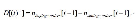
(1) |
|
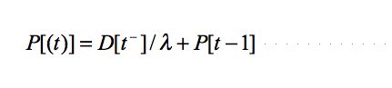
(2) |
|
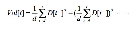
(3) |
|
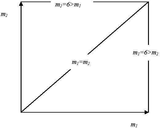
| Figure 1. Three configurations of historical memories |
| Table 1: Correlations among R1, R2 and Vol1 when m2=6, and m1 increases from 1 to 6 | |||
| R 1 | R 2 | Vol1 | |
| R 1 | 1 | ||
| R 2 | 0.982 | 1 | |
| Vol1 | 0.985 | 0.996 | 1 |
| Table 2: Correlations among R1, R2 and Vol2 when m1=6, and m2 increases from 1 to 6 | |||
| R1 | R2 | Vol2 | |
| R1 | 1 | ||
| R2 | -0.246 | 1 | |
| Vol2 | 0.148 | -0.892 | 1 |
| Table 3: Correlations among R1, R2 and Vol3 when m1=m2, and they increase from 1 to 6 | |||
| R1 | R2 | Vol3 | |
| R1 | 1 | ||
| R2 | 0.977 | 1 | |
| Vol3 | -0.859 | -0.737 | 1 |
|
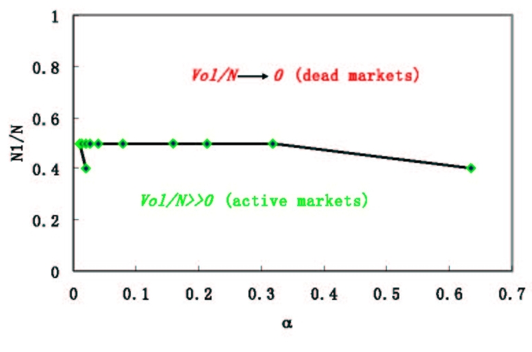
| Figure 2. Two-phase phenomenon of local volatilities under simulation condition of m1 < m2, where α = 2m1 / N |
|
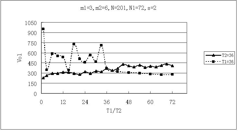
| Figure 3. Relations between means of local volatilities and time horizon T1 (T2) when T2=36 (T1=36), m1=3, m2=6, N=201, N1=72 and s=2 |
|
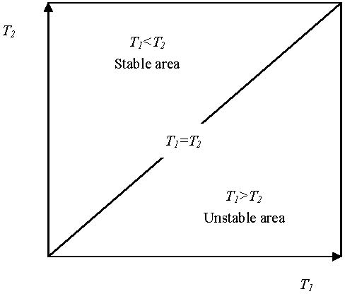
| Figure 4. Two-phase phenomenon of local volatilities in T1-T2 space under simulation condition of m1=3, m2=6, N=201, N1=72 and s=2 |
|
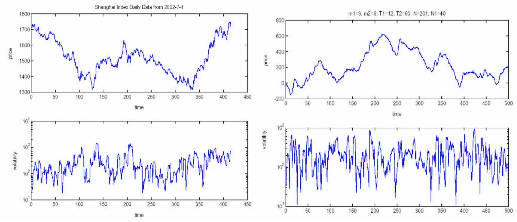
| Figure 5. Time series and local volatilities of Shanghai Index daily data and the mix-game with parameters of m1=3, m2=6, T1=12, T2=60, N=201, N1=40 and s=2 |
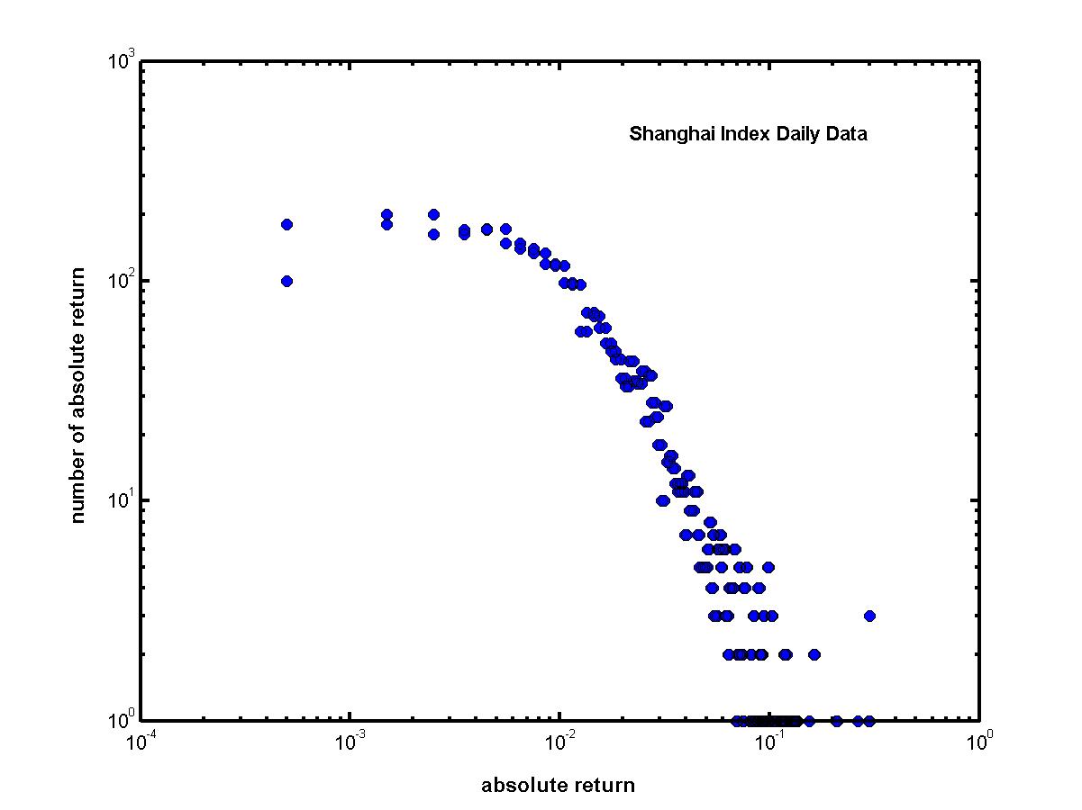 |
| Figure 6. Log-log plot of Shanghai Index daily absolute returns that is non-Gaussian (Yang 2004) |
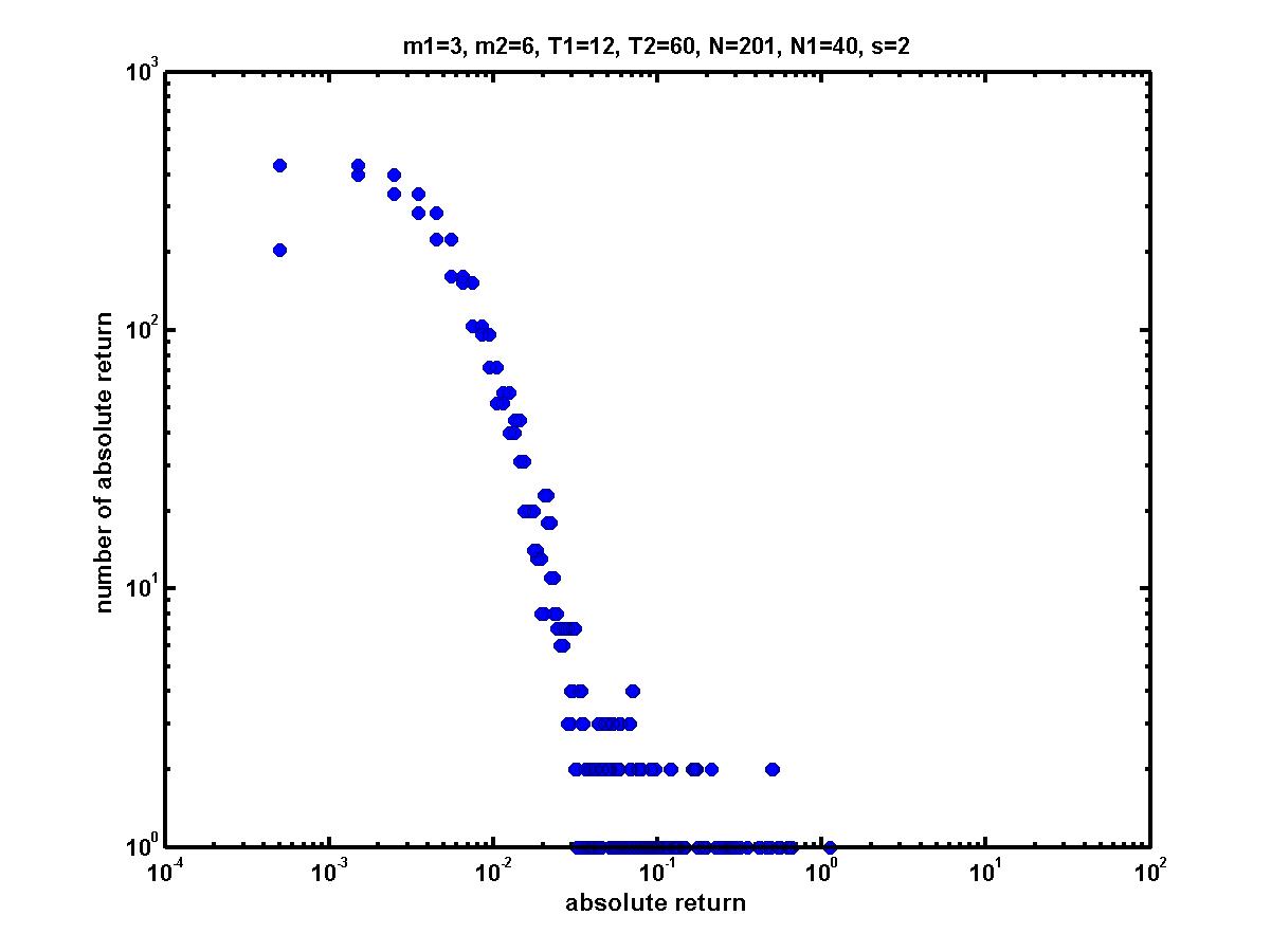 |
| Figure 7. Log-log plot of the mix-game absolute returns with parameters of m1=3, m2=6, T1=12, T2=60, N=201, N1=40 and s=2 |
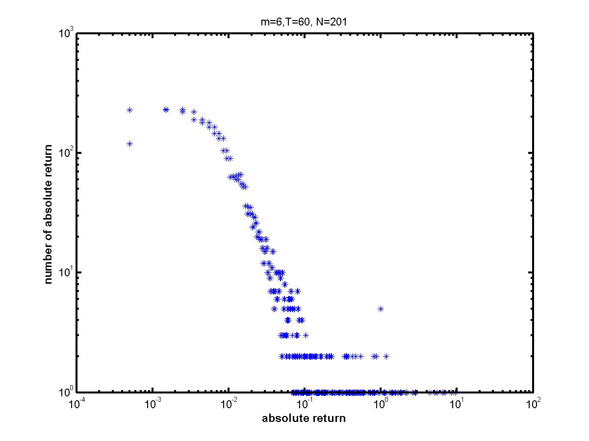 |
| Figure 8. Log-log plot of the MG absolute returns with parameters of m=6, T=60 and N=201 and s=2 |
|
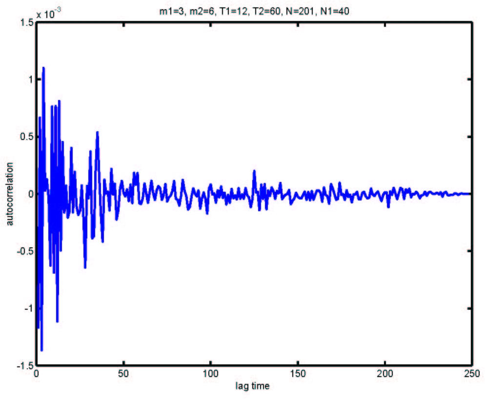
| Figure 9. Autocorrelations of logarithmic returns of the mix-game with m1=3, T1=12, m2=6, T2=60, N1=40, N=201 and s=2 |
| Table 4: A sample of agent's strategies (m=2) | |
| Historical information | prediction |
| 00 | 1 |
| 01 | 0 |
| 10 | 0 |
| 11 | 1 |
BOUCHAUD J.P. and Cont, R. (1998) Eur. Phys. J. B 6 543.
CHALLET, D. and Zhang, Y. C. (1997) Phyisca A 246, 407.
COOLEN A C C (2005) The Mathematical Theory of Minority Games, Oxford University Press, Oxford.
FARMER J.D. (2002) Industrial and Corporate Change vol. 11, 895-953.
GOU C. (2005) arXiv:physics/0508056.
GOU C. (2006) Chinese Physics 15 1239.
JEFFERIES P. and Johnson N. F. (2001) Oxford Center for Computational Finance working paper: OCCF/010702.
JOHNSON N. F., Hui P. M., Zheng D. and Hart M. (1999) J. Phys. A: Math. Gen. 32 L427-L431.
JOHNSON Neil F.,Jefferies P., and Hui P. M. (2003) Financial Market Complexity, Oxford University Press, Oxford.
JUDD K.L. and Tesfatsion L. edited (2005) Handbook of Computational Economics, Volume 2: Agent-Based Computational Economics, Elsevier Science B.V.
LUNA F. and Perrone A. edited (2002) Agent-based Methods in Economics and Finance: Sinulations in Swarm, Kluwer Academic Publisher, Norwell, Massachusetts.
LUX T. (1995) Economic Journal 105 881
LUX T. and Marchesi M. (1999) Nature 397 498
MARSILI M. (2001) Physica A 299 93.
SHLEIFER A. (2000) Inefficient Markets: an Introduction to Behavioral Financial, Oxford University Press, Oxford, UK.
YANG C. (2004) thesis of Beijing University of Aeronautics and Astronautics.
 Return to Contents of this issue
© Copyright Journal of Artificial Societies and Social Simulation, [2006]