
Matteo Richiardi (2004)
Generalizing Gibrat: Reasonable Multiplicative Models of Firm Dynamics
Journal of Artificial Societies and Social Simulation
vol. 7, no. 1
To cite articles published in the Journal of Artificial Societies and Social Simulation, please reference the above information and include paragraph numbers if necessary
<https://www.jasss.org/7/1/2.html>
Received: 24-Mar-2003 Accepted: 23-Jul-2003 Published: 31-Jan-2004
 Abstract
| P[X = x] ~ x-(k+1) = x-a | (1) |
| P[X > x] ~ x-k | (2) |
| yi ~ ri-b, with b close to unity | (3) |
has found many applications, in particular to the study of city size distribution, where it is known to be surprisingly robust and stable.
| St+1 = λ t St | (4) |
Taking logs, this model reduces to
| lnSt+1 = Σ ln λt | (5) |
| St+1 = λtSt + ρ t | (6) |
This model defines a stationary process if E(lnSt) < 0. Moreover, if St sometimes takes values larger than one (intermittent amplifications) and the (constant or stochastic) additive term is not null, the process leads to a power-law pdf.
|
(7) |
| St+1 = exp( F(x), {λt, ρt,...}λt xt | (8) |
such that F → 0 for large St (thus leading to a 'pure' multiplicative process) and F → ∞ for St → 0 (repulsion from the origin). With some additional constraints on F, this class of processes has a power-law pdf.
|
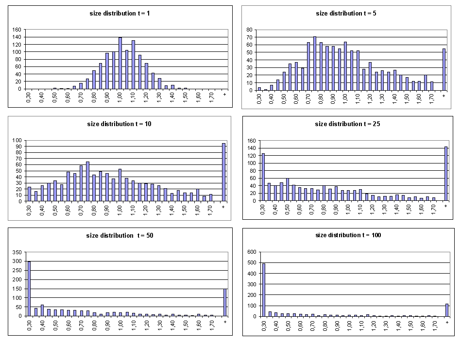
| Figure 1. Evolution of firm size distribution with λ ~ N (1, 0.15) |
|
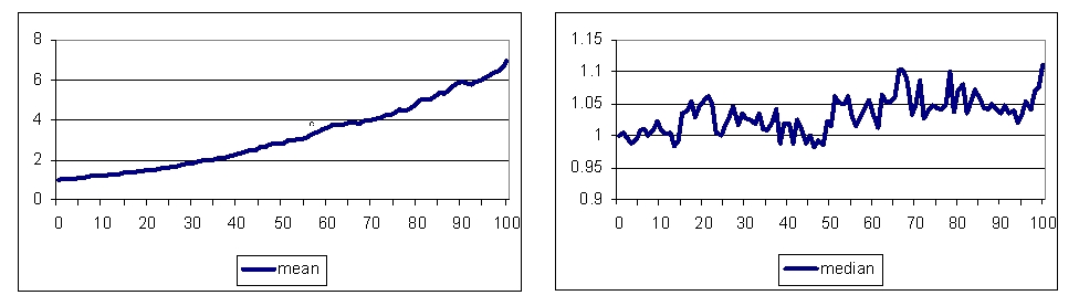
| Figure 2. Evolution of firm size mean and median with ln λ ~ N (1, 0.20) |
|
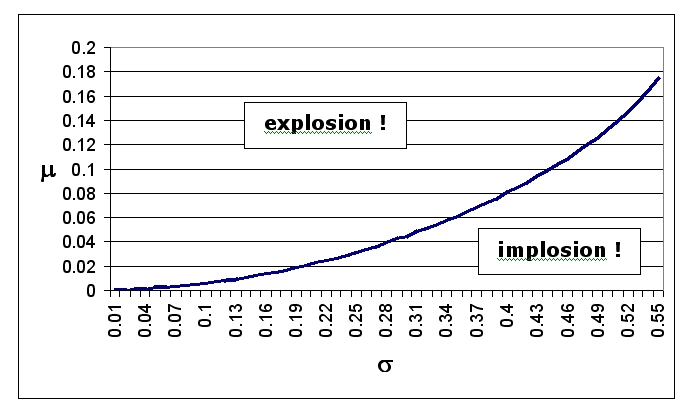
| Figure 3. Median stationarity in a pure Gibrat model |
|
(9) |
|
(10) |
where D1/2, t is the lower half of the (empirical) firm size distribution at time t.
|
(11) |
|
(12) |
where S* is the optimal size of the market, i.e. the dimension that keep supply and (exogenous) demand in equilibrium, given (exogenous) prices, and D1/2, t is the lower half of the (empirical) firm size distribution at time t.
| Table 1: Entry and exit mechanisms | ||
| ENTRY | EXIT | |
| NON-THRESHOLD | · Proportional Number · Proportional Dimension | · Minimum Size · Proportional Number |
| THRESHOLD | · Excess Demand | · Excess Supply Affects All · Excess Supply Affects Small · Excess Supply Affects Large |
| Entry mechanism: | Excess Demand |
| Exit mechanism: | Excess Supply Affects All |
| Initial number of firms: | 100 |
| Maximum sector dimension: | 300 |
| α: | 1.0 (Take-up rate) |
| μ: | 0.1 |
| σ: | 0.1 |
| m: | 1.0 (mean heteroskedasticity) |
| s: | 0.0 (variance homoskedasticity) |
|
|
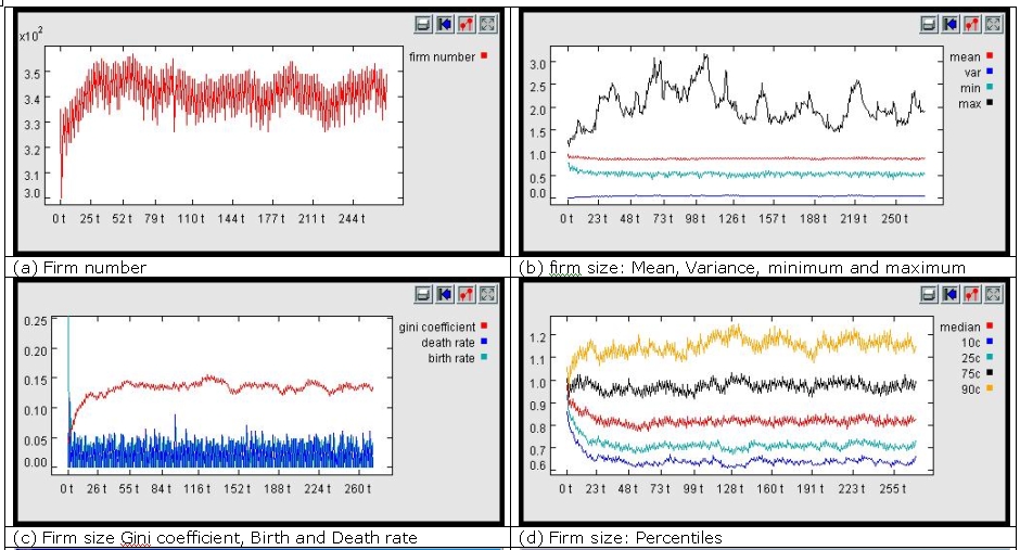
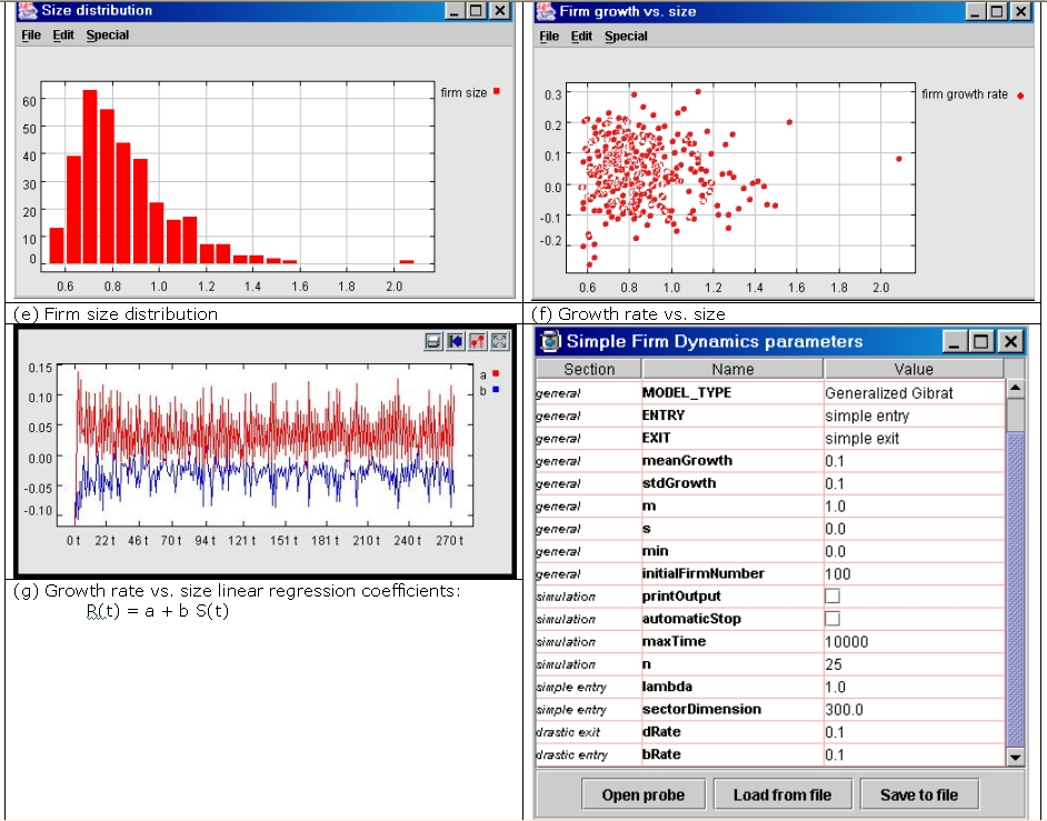
| Figure 4. Simulation output |
|
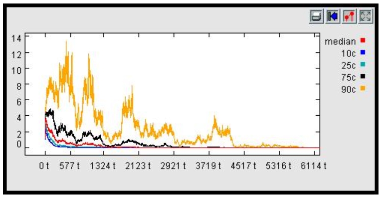
| Figure 5. Example of firm size distribution when long-run stopping mechanisms don't work (single simulation run) |
|
| Figure 6. Long-run dynamics, mean heteroskedasticity (multiple simulation runs) |
|
| Figure 7. Example of firm size distribution, mean heteroskedasticity (single simulation run) |
|
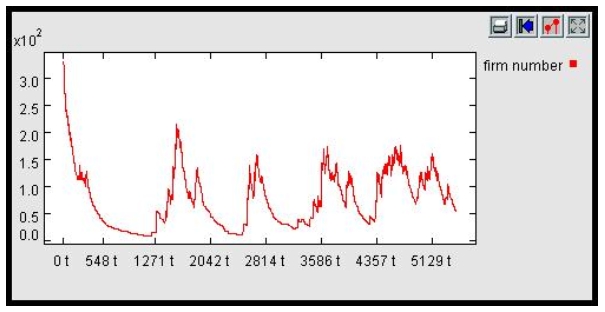
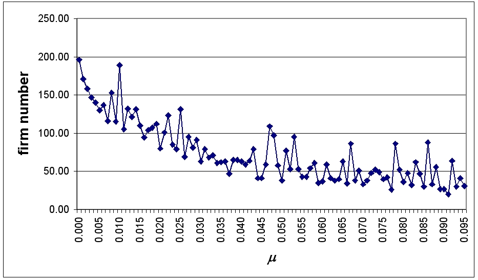
| Figure 8. Total firm number with positive minimum size, zero average growth and Excess Demand entry (single simulation run) |
|
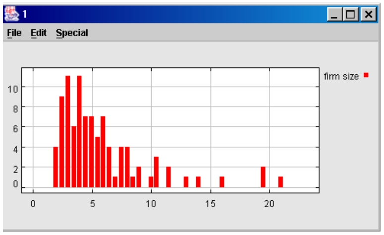
| Figure 9. Firm size distribution with Excess Supply Affects All exit mechanism, 0 minimum size and μ = 0.2 |
With positive minimum size this risk is avoided.
|
| Figure 10. Long run dynamics, Excess Demand entry and Excess Supply Affects All exit |
| Table 2: Model outcomes | ||||||
| Entry | ||||||
| Exit | Gibrat | NON-THRESHOLD | THRESHOLD | |||
| No entry | Proportional Number | Proportional Dimension (*) | Excess Demand | |||
| Gibrat | No exit | implosion explosion | implosion explosion | - | R-distribution (*) explosion | |
| NON-THRESHOLD | Minimum Size | implosion explosion | implosion explosion | implosion explosion | R-distribution (*) explosion | |
| Proportional Number | implosion monopoly | implosion explosion/monopoly | implosion explosion | R-distribution (*) monopoly | ||
| THRESHOLD | Excess Supply Affects Small | implosion monopoly | implosion monopoly | implosion explosion | R-distribution (*) monopoly | |
| Excess Supply Affects Large | implosion monopoly | implosion monopoly | implosion R-distribution | R-distribution (*) monopoly | ||
| Excess Supply Affects All | implosion monopoly | implosion R-distribution (*) | implosion R-distribution | R-distribution (*) R-distribution (*) | ||
Implosion means firm size converging to zero, or firm number converging to zero given non-increasing firm size
Explosion means firm size growing indefinitely, or firm number growing indefinitely given non-collapsing firm size
When a Monopoly is reached, the remaining firm keeps growing indefinitely
All combinations were simulated. Results not reported in the Appendix are available upon request.
2 See Sutton (1997) for a survey on the developments of these models
3 Indeed, if the variance of a lognormal distribution is large, it may appear like a power-law distribution for several orders of magnitude (Mitzenmacher 2001).
4 In particular, they show that the appearance of the scaling power-laws is as generic in multiplicative stochastic systems as the Boltzmann law is in additive stochastic systems
5 Redner (1990) notes that <<[a] crucial feature of the process is that extreme events, although exponentially rare in n, are exponentially different from the typical, or most probable value of the product>>.
6 Simulation results for Blank and Solomon model are presented in section 6
7 This feature also allows model calibration, if needed.
8 Since Proportional Dimension entry mechanism requires new firms size to be equal to the minimum size, this cannot be 0. So, in considering Proportional Dimension entry the minimum size has to be raised, and Minimum Size exit also considered (firms below minimum size exit the market), thus reproducing Blank & Solomon model.
9 The only exception, among the entry mechanisms considered here, is Proportional Dimension (Blank & Solomon 2000). In this case however, the combination of entry and exit mechanisms is simply incoherent, because threshold exit mechanisms imply a reduction in the number of firms in the market when capacity grows above the threshold, while Proportional Dimension entry implies an increase in the number of firms as total capacity increases. Which one predominates depends on the particular event schedule implemented in the simulation.
10 but as long as some new firms are allowed to enter the market. Otherwise, with exit but without entry, the system obviously moves towards a monopoly.
Parameter values were drawn randomly within the range of interest. In general, the growth rate mean goes from –0.02 to 0.2; the growth rate standard deviation from 0.1 to 0.2; the minimum size from 0 to 0.5; the birth rate from 0 to 0.1 (when not specified, it is fixed at 0.1). Particularly interesting subsets of the parameter space were over-investigated.
Each simulation can stop because:
| Table A.1: Simulation results for Minimum Size exit and Proportional Dimension entry (Blank & Solomon 2000), mean and variance homoskedasticity | |||||||
| time | meanGrowth | stdGrowth | minSize | k | meanSize | varSize | firmNumber |
| 144 | - 0.019 | 0.100 | 0.369 | 0.088 | - | - | - |
| 190 | - 0.017 | 0.162 | 0.244 | 0.001 | - | - | - |
| 190 | - 0.016 | 0.155 | 0.410 | 0.026 | - | - | - |
| 184 | - 0.016 | 0.130 | 0.205 | 0.039 | - | - | - |
| 429 | - 0.015 | 0.114 | 0.187 | 0.013 | - | - | - |
| 566 | - 0.010 | 0.115 | 0.042 | 0.084 | - | - | - |
| 582 | - 0.009 | 0.101 | 0.331 | 0.057 | - | - | - |
| 811 | - 0.007 | 0.166 | 0.048 | 0.073 | - | - | - |
| 718 | - 0.004 | 0.130 | 0.446 | 0.030 | - | - | - |
| 654 | - 0.002 | 0.121 | 0.184 | 0.036 | - | - | - |
| 3209 | 0.004 | 0.164 | 0.239 | 0.077 | 3.208 | 20,788.608 | 10,000 |
| 736 | 0.007 | 0.128 | 0.046 | 0.048 | 2.391 | 15,597.058 | 10,000 |
| 541 | 0.010 | 0.128 | 0.090 | 0.020 | 3.466 | 3,854.679 | 10,000 |
| 595 | 0.013 | 0.193 | 0.225 | 0.001 | 4.357 | 16,559.634 | 10,000 |
| 304 | 0.017 | 0.140 | 0.013 | 0.036 | 3.233 | 14,043.853 | 10,000 |
| 242 | 0.021 | 0.159 | 0.494 | 0.097 | 4.241 | 3,634.481 | 10,000 |
| 254 | 0.021 | 0.110 | 0.129 | 0.033 | 3.350 | 1,779.483 | 10,000 |
| 212 | 0.024 | 0.180 | 0.343 | 0.091 | 4.075 | 3,653.648 | 10,000 |
| 156 | 0.027 | 0.104 | 0.289 | 0.093 | 2.986 | 570.287 | 10,000 |
| 157 | 0.031 | 0.139 | 0.219 | 0.072 | 3.387 | 692.511 | 10,000 |
| 119 | 0.032 | 0.178 | 0.483 | 0.029 | 3.477 | 1,642.138 | 10,000 |
| 125 | 0.033 | 0.113 | 0.334 | 0.093 | 2.647 | 210.094 | 10,000 |
| 120 | 0.038 | 0.133 | 0.312 | 0.056 | 2.695 | 395.503 | 10,000 |
| 119 | 0.039 | 0.118 | 0.038 | 0.033 | 2.324 | 708.301 | 10,000 |
| 95 | 0.040 | 0.127 | 0.390 | 0.045 | 2.509 | 322.448 | 10,000 |
| 101 | 0.041 | 0.181 | 0.454 | 0.030 | 2.981 | 395.599 | 10,000 |
| 101 | 0.041 | 0.162 | 0.363 | 0.046 | 2.895 | 652.151 | 10,000 |
| 109 | 0.042 | 0.112 | 0.085 | 0.035 | 2.170 | 820.554 | 10,000 |
| 91 | 0.048 | 0.101 | 0.026 | 0.053 | 1.948 | 457.778 | 10,000 |
| 93 | 0.050 | 0.190 | 0.181 | 0.092 | 2.703 | 4,772.303 | 10,000 |
| 82 | 0.057 | 0.106 | 0.023 | 0.068 | 1.823 | 292.299 | 10,000 |
| 61 | 0.057 | 0.107 | 0.315 | 0.038 | 1.778 | 69.647 | 10,000 |
| 61 | 0.065 | 0.114 | 0.186 | 0.062 | 1.753 | 119.713 | 10,000 |
| 63 | 0.066 | 0.132 | 0.167 | 0.058 | 1.810 | 206.126 | 10,000 |
| 60 | 0.067 | 0.132 | 0.190 | 0.066 | 1.863 | 111.348 | 10,000 |
| 69 | 0.067 | 0.122 | 0.010 | 0.028 | 1.764 | 431.344 | 10,000 |
| 52 | 0.067 | 0.157 | 0.401 | 0.095 | 2.025 | 81.031 | 10,000 |
| 55 | 0.069 | 0.123 | 0.262 | 0.049 | 1.715 | 55.592 | 10,000 |
| 57 | 0.071 | 0.183 | 0.263 | 0.100 | 2.163 | 228.262 | 10,000 |
| 48 | 0.081 | 0.145 | 0.247 | 0.026 | 1.758 | 76.322 | 10,000 |
| 50 | 0.084 | 0.193 | 0.152 | 0.065 | 1.978 | 254.309 | 10,000 |
| 48 | 0.089 | 0.191 | 0.179 | 0.084 | 1.966 | 184.449 | 10,000 |
| 42 | 0.090 | 0.193 | 0.392 | 0.071 | 1.935 | 46.714 | 10,000 |
| 38 | 0.092 | 0.128 | 0.285 | 0.020 | 1.532 | 34.855 | 10,000 |
| 39 | 0.093 | 0.128 | 0.280 | 0.094 | 1.523 | 31.653 | 10,000 |
| 48 | 0.093 | 0.165 | 0.064 | 0.093 | 1.754 | 272.310 | 10,000 |
| 37 | 0.094 | 0.113 | 0.256 | 0.096 | 1.418 | 25.878 | 10,000 |
| 43 | 0.095 | 0.117 | 0.098 | 0.074 | 1.442 | 74.375 | 10,000 |
| 46 | 0.095 | 0.125 | 0.037 | 0.061 | 1.477 | 115.729 | 10,000 |
| 29 | 0.099 | 0.131 | 0.481 | 0.060 | 1.506 | 10.518 | 10,000 |
| 38 | 0.100 | 0.149 | 0.240 | 0.056 | 1.610 | 50.363 | 10,000 |
The system generally either becomes extinct, or explodes in the number of firms. Only by appropriately choosing values for the average growth rate very close to zero, does it look stationary
| Table A.2: Simulation results for Proportional Number entry, mean and variance homoskedasticity | ||||||
| time | meanGrowth | stdGrowth | birthRate | meanSize | varSize | firmNumber |
| 113 | -0.0199 | 0.1407 | 0.0365 | 0.007073119 | 1.31E-03 | 10000 |
| 50 | -0.0149 | 0.1055 | 0.0813 | 0.113285536 | 1.21E-02 | 10000 |
| 47 | -0.0122 | 0.1023 | 0.0879 | 0.145749252 | 1.93E-02 | 10000 |
| 46 | -0.0104 | 0.15 | 0.0881 | 0.094486148 | 4.30E-02 | 10000 |
| 44 | -0.0076 | 0.1318 | 0.0922 | 0.144882328 | 3.96E-02 | 10000 |
| 366 | -0.0075 | 0.1824 | 0.0122 | 2.87E-04 | 6.25E-05 | 10000 |
| 245 | -0.0071 | 0.1565 | 0.0176 | 0.003809768 | 0.003164975 | 10000 |
| 5000 | -0.0069 | 0.155 | 0.0005 | 4.53E-32 | 1.94E-61 | 100 |
| 194 | -0.0066 | 0.103 | 0.0216 | 0.019709888 | 1.25E-02 | 10000 |
| 60 | -0.0037 | 0.1231 | 0.0684 | 0.139585452 | 7.20E-02 | 10000 |
| 341 | -0.0034 | 0.1077 | 0.0131 | 0.012854722 | 1.72E-02 | 10000 |
| 63 | -0.0033 | 0.1413 | 0.0649 | 0.087967898 | 5.63E-02 | 10000 |
| 108 | -0.0015 | 0.1143 | 0.038 | 0.108112195 | 2.02E-01 | 10000 |
| 375 | -0.0013 | 0.1923 | 0.012 | 0.002633735 | 3.57E-03 | 10000 |
| 84 | 0.0014 | 0.1918 | 0.0484 | 0.060633785 | 7.06E-01 | 10000 |
| 46 | 0.0026 | 0.1277 | 0.0891 | 0.228038483 | 8.03E-02 | 10000 |
| 49 | 0.0042 | 0.1868 | 0.0837 | 0.106101557 | 2.05E-01 | 10000 |
| 60 | 0.0052 | 0.1288 | 0.0674 | 0.237871611 | 1.43E-01 | 10000 |
| 53 | 0.006 | 0.1116 | 0.0775 | 0.328486402 | 1.27E-01 | 10000 |
| 5000 | 0.0073 | 0.112 | 0.0035 | 8.99E+07 | 7.97E+17 | 100 |
| 72 | 0.0076 | 0.1992 | 0.0571 | 0.109641713 | 1.37E+00 | 10000 |
| 5000 | 0.0125 | 0.1221 | 0.0021 | 1.94E+19 | 3.32E+40 | 100 |
| 232 | 0.0145 | 0.1339 | 0.0185 | 1.465814644 | 232.1458876 | 10000 |
| 5000 | 0.0151 | 0.141 | 0.0032 | 1.15E+19 | 1.29E+40 | 100 |
| 5000 | 0.0169 | 0.1912 | 0.0092 | 9.33E+10 | 8.68E+23 | 100 |
| 301 | 0.0178 | 0.199 | 0.0146 | 2.610688082 | 4.66E+03 | 10000 |
| 86 | 0.0191 | 0.1142 | 0.0478 | 0.748169033 | 2.12225235 | 10000 |
| 49 | 0.0198 | 0.1643 | 0.0829 | 0.408440377 | 0.701304711 | 10000 |
| 61 | 0.022 | 0.1794 | 0.0667 | 0.348275489 | 9.23E+00 | 10000 |
| 5000 | 0.0227 | 0.1224 | 0.0064 | 4.23E+39 | 1.21E+81 | 100 |
| 43 | 0.0279 | 0.1405 | 0.0967 | 0.625611697 | 8.91E-01 | 10000 |
| 77 | 0.0288 | 0.1941 | 0.0529 | 0.7237275 | 4.55E+01 | 10000 |
| 66 | 0.0297 | 0.1019 | 0.0622 | 1.721070697 | 3.89E+00 | 10000 |
| 103 | 0.0328 | 0.1318 | 0.0398 | 2.926515182 | 1.34E+02 | 10000 |
| 5000 | 0.0348 | 0.1275 | 0.0012 | 4.62E+68 | 2.14E+139 | 100 |
| 160 | 0.0371 | 0.1456 | 0.0261 | 11.4366613 | 3287.954539 | 10000 |
| 54 | 0.0383 | 0.1751 | 0.0762 | 0.842794132 | 5.93E+00 | 10000 |
| 61 | 0.0391 | 0.186 | 0.0669 | 0.787607046 | 1.75E+01 | 10000 |
| 159 | 0.0392 | 0.1347 | 0.0262 | 25.84512331 | 3.52E+04 | 10000 |
| 104 | 0.0418 | 0.1236 | 0.0394 | 8.122864781 | 5.67E+02 | 10000 |
| 155 | 0.0451 | 0.1125 | 0.0269 | 89.0935399 | 2.18E+05 | 10000 |
| 66 | 0.0453 | 0.1369 | 0.0621 | 2.609594454 | 4.61E+01 | 10000 |
| 46 | 0.0476 | 0.1498 | 0.0887 | 1.557484775 | 7.07E+00 | 10000 |
| 162 | 0.0479 | 0.1416 | 0.0258 | 100.7326391 | 7.49E+05 | 10000 |
| 97 | 0.0514 | 0.1812 | 0.0421 | 6.102945117 | 1.65E+03 | 10000 |
| 76 | 0.0518 | 0.1758 | 0.0537 | 3.102340484 | 1.78E+02 | 10000 |
| 313 | 0.0546 | 0.1214 | 0.0142 | 457849.6943 | 3.54E+13 | 10000 |
| 62 | 0.0555 | 0.1078 | 0.0666 | 6.555210396 | 5.60E+01 | 10000 |
| 5000 | 0.0564 | 0.1998 | 0.0011 | 3.72E+90 | 1.10E+183 | 100 |
| 5000 | 0.0598 | 0.196 | 0.0052 | 4.42E+98 | 8.90E+198 | 100 |
| 5000 | 0.0649 | 0.1001 | 0.0034 | 2.19E+132 | 2.81E+266 | 100 |
| 173 | 0.0656 | 0.1831 | 0.0243 | 1515.77226 | 4.53E+08 | 10000 |
| 47 | 0.0657 | 0.1432 | 0.0876 | 3.507168094 | 2.79E+01 | 10000 |
| 177 | 0.0675 | 0.1008 | 0.0238 | 10640.51041 | 1.04E+09 | 10000 |
| 188 | 0.0679 | 0.1917 | 0.0224 | 10915.37818 | 1.84E+11 | 10000 |
| 5000 | 0.0729 | 0.151 | 0.0033 | 4.35E+139 | 6.93E+280 | 100 |
| 89 | 0.0734 | 0.1317 | 0.0462 | 67.69909378 | 2.99E+04 | 10000 |
| 219 | 0.0751 | 0.1405 | 0.0193 | 336439.7406 | 5.48E+12 | 10000 |
| 41 | 0.0756 | 0.1797 | 0.0995 | 3.437785585 | 3.76E+01 | 10000 |
| 41 | 0.0762 | 0.1268 | 0.0999 | 6.15519068 | 33.57587775 | 10000 |
| 46 | 0.0847 | 0.1147 | 0.0889 | 12.80794819 | 1.37E+02 | 10000 |
| 211 | 0.0864 | 0.1308 | 0.02 | 1674692.651 | 1.57E+14 | 10000 |
| 102 | 0.092 | 0.1782 | 0.04 | 508.8034846 | 1.10E+07 | 10000 |
| 48 | 0.0921 | 0.1583 | 0.086 | 11.96688222 | 502.5483125 | 10000 |
| 122 | 0.0934 | 0.1312 | 0.0338 | 5913.84004 | 4.94E+09 | 10000 |
| 169 | 0.0954 | 0.1291 | 0.0248 | 265109.8097 | 1.46E+12 | 10000 |
| 48 | 0.0956 | 0.1334 | 0.085 | 18.16608091 | 4.57E+02 | 10000 |
| 129 | 0.0968 | 0.1843 | 0.0319 | 7027.572723 | 6.67E+09 | 10000 |
| 49 | 0.0969 | 0.178 | 0.0825 | 15.14853015 | 1.54E+03 | 10000 |
| 101 | 0.0985 | 0.1596 | 0.0405 | 1205.134053 | 2.13E+07 | 10000 |
| 54 | 0.0996 | 0.1986 | 0.0756 | 16.87269573 | 4.31E+03 | 10000 |
The system either implodes in size, or explodes in size or in the number of firms
| Table A.3: Simulation results for Excess Demand entry, mean and variance homoskedasticity | ||||||
| time | meanGrowth | stdGrowth | minSize | meanSize | varSize | firmNumber |
| 86 | - 0.017 | 0.183390165 | 0.00 | 0.0 | 8.32E-01 | 10000 |
| 102 | - 0.016 | 0.117801847 | 0.00 | 0.0 | 7.01E-03 | 10000 |
| 88 | - 0.015 | 0.169921587 | 0.00 | 0.0 | 5.64E-02 | 10000 |
| 105 | - 0.014 | 0.15744653 | 0.00 | 0.0 | 7.38E-02 | 10000 |
| 140 | - 0.007 | 0.135999785 | 0.00 | 0.0 | 5.42E-02 | 10000 |
| 185 | - 0.004 | 0.134036494 | 0.00 | 0.0 | 8.10E-02 | 10000 |
| 276 | - 0.002 | 0.145608349 | 0.00 | 0.0 | 3.31E-01 | 10000 |
| 521 | 0.001 | 0.173816895 | 0.00 | 0.0 | 1.35E+00 | 10000 |
| 1971 | 0.003 | 0.136858843 | 0.00 | 0.0 | 2.53E+00 | 10000 |
| 407 | 0.005 | 0.180479 | 0.00 | 0.0 | 8.44E-01 | 10000 |
| 878 | 0.005 | 0.162632365 | 0.00 | 0.0 | 7.59E-01 | 10000 |
| 774 | 0.005 | 0.187372841 | 0.00 | 0.0 | 8.06E-01 | 10000 |
| 5000 | 0.007 | 0.132841394 | 0.00 | 986.1 | 8.71E+07 | 326 |
| 1983 | 0.008 | 0.110686137 | 0.00 | 1060388.9 | 2.30E+14 | 326 |
| 1102 | 0.010 | 0.137889921 | 0.00 | 1048316.0 | 2.55E+14 | 319 |
| 1708 | 0.012 | 0.140865172 | 0.00 | 1066578.4 | 2.23E+14 | 311 |
| 1052 | 0.014 | 0.105100224 | 0.00 | 1008348.9 | 7.31E+13 | 305 |
| 1423 | 0.015 | 0.197298795 | 0.00 | 1022229.7 | 3.32E+14 | 318 |
| 1209 | 0.017 | 0.166114255 | 0.00 | 1060477.9 | 6.89E+13 | 305 |
| 786 | 0.019 | 0.107521161 | 0.00 | 1009923.2 | 1.46E+13 | 306 |
| 635 | 0.021 | 0.100813935 | 0.00 | 1047619.5 | 6.55E+13 | 318 |
| 603 | 0.024 | 0.136851006 | 0.00 | 1006363.1 | 3.58E+13 | 320 |
| 596 | 0.026 | 0.146662735 | 0.00 | 1016119.3 | 4.47E+13 | 309 |
| 545 | 0.030 | 0.177885087 | 0.00 | 1075796.0 | 9.51E+13 | 299 |
| 500 | 0.030 | 0.136751732 | 0.00 | 1040911.1 | 2.40E+13 | 323 |
| 460 | 0.034 | 0.178484828 | 0.00 | 1001656.5 | 4.87E+13 | 302 |
| 379 | 0.037 | 0.143598034 | 0.00 | 1106669.3 | 7.84E+13 | 304 |
| 353 | 0.038 | 0.199081417 | 0.00 | 1027488.1 | 2.69E+14 | 304 |
| 381 | 0.038 | 0.147913122 | 0.00 | 1005277.6 | 4.38E+13 | 296 |
| 375 | 0.038 | 0.152318634 | 0.00 | 1096690.3 | 7.07E+13 | 305 |
| 369 | 0.039 | 0.108664023 | 0.00 | 1041130.8 | 9.67E+12 | 300 |
| 338 | 0.042 | 0.101374458 | 0.00 | 1009610.9 | 8.70E+12 | 295 |
| 297 | 0.046 | 0.186618452 | 0.00 | 1000945.5 | 1.38E+14 | 301 |
| 305 | 0.048 | 0.136860176 | 0.00 | 1019298.9 | 1.20E+13 | 297 |
| 283 | 0.051 | 0.126433815 | 0.00 | 1037268.2 | 5.67E+12 | 287 |
| 241 | 0.061 | 0.176564235 | 0.00 | 1041227.7 | 2.03E+13 | 297 |
| 232 | 0.062 | 0.160566786 | 0.00 | 1010452.3 | 1.34E+13 | 295 |
| 213 | 0.066 | 0.122797088 | 0.00 | 1022044.0 | 1.20E+13 | 289 |
| 211 | 0.068 | 0.190573817 | 0.00 | 1015530.1 | 3.06E+13 | 300 |
| 202 | 0.069 | 0.115458192 | 0.00 | 1011232.1 | 1.24E+13 | 281 |
| 199 | 0.071 | 0.140121704 | 0.00 | 1007669.2 | 9.08E+12 | 278 |
| 198 | 0.073 | 0.166998349 | 0.00 | 1011510.1 | 1.72E+13 | 286 |
| 199 | 0.073 | 0.168185148 | 0.00 | 1007171.7 | 1.95E+13 | 291 |
| 191 | 0.078 | 0.173193092 | 0.00 | 1143654.1 | 3.83E+13 | 284 |
| 183 | 0.079 | 0.179915633 | 0.00 | 1047905.9 | 1.55E+13 | 281 |
| 174 | 0.081 | 0.143656232 | 0.00 | 1044834.6 | 1.02E+13 | 277 |
| 172 | 0.085 | 0.196514968 | 0.00 | 1024234.7 | 3.81E+13 | 283 |
| 164 | 0.087 | 0.158574015 | 0.00 | 1133015.1 | 2.23E+13 | 277 |
| 161 | 0.092 | 0.155774591 | 0.00 | 1014843.3 | 6.52E+12 | 283 |
| 148 | 0.095 | 0.121072573 | 0.00 | 1001135.8 | 3.11E+13 | 270 |
| time | meanGrowth | stdGrowth | minSize | meanSize | varSize | firmNumber |
| 5000 | - 0.017 | 0.174937733 | 0.46 | 1.2 | 1.53E+00 | 236 |
| 5000 | - 0.017 | 0.157630062 | 0.29 | 0.5 | 9.15E-02 | 489 |
| 5000 | - 0.015 | 0.167134407 | 0.05 | 0.1 | 1.16E-02 | 1647 |
| 5000 | - 0.014 | 0.146423363 | 0.35 | 0.7 | 2.62E-01 | 393 |
| 5000 | - 0.012 | 0.151384946 | 0.42 | 1.0 | 8.42E-01 | 297 |
| 5000 | - 0.009 | 0.191627284 | 0.24 | 0.7 | 5.56E-01 | 421 |
| 5000 | - 0.005 | 0.175235791 | 0.03 | 0.1 | 7.46E-02 | 1972 |
| 5000 | - 0.005 | 0.135787397 | 0.36 | 1.5 | 1.75E+01 | 205 |
| 5000 | - 0.001 | 0.157757404 | 0.25 | 1.1 | 2.82E+00 | 280 |
| 5000 | 0.005 | 0.180028131 | 0.15 | 4.9 | 5.40E+02 | 107 |
| 5000 | 0.007 | 0.167542556 | 0.46 | 5.9 | 2.80E+02 | 59 |
| 5000 | 0.008 | 0.193803277 | 0.15 | 4.2 | 1.05E+02 | 74 |
| 1349 | 0.010 | 0.10404251 | 0.30 | 1063150.0 | 1.42E+14 | 184 |
| 2741 | 0.010 | 0.149947068 | 0.16 | 1043546.1 | 9.14E+12 | 25 |
| 2006 | 0.011 | 0.145633403 | 0.09 | 1081066.5 | 4.45E+13 | 103 |
| 1094 | 0.012 | 0.143763984 | 0.04 | 1065803.0 | 1.98E+14 | 184 |
| 1355 | 0.012 | 0.183116142 | 0.22 | 1064620.7 | 1.52E+13 | 14 |
| 606 | 0.024 | 0.102594689 | 0.36 | 1013401.6 | 9.70E+12 | 294 |
| 527 | 0.028 | 0.15830852 | 0.40 | 1054555.2 | 9.98E+13 | 209 |
| 551 | 0.029 | 0.163590133 | 0.21 | 1000182.7 | 3.79E+13 | 268 |
| 479 | 0.031 | 0.134963877 | 0.42 | 1017652.7 | 2.13E+13 | 275 |
| 485 | 0.031 | 0.131929416 | 0.09 | 1007541.0 | 1.81E+13 | 303 |
| 398 | 0.036 | 0.11595775 | 0.47 | 1037959.6 | 1.26E+13 | 284 |
| 391 | 0.037 | 0.115712528 | 0.49 | 1020198.6 | 1.15E+13 | 289 |
| 374 | 0.039 | 0.141035212 | 0.32 | 1029554.1 | 2.19E+13 | 295 |
| 336 | 0.045 | 0.177942767 | 0.16 | 1001148.2 | 3.00E+13 | 289 |
| 328 | 0.045 | 0.159032862 | 0.04 | 1021096.0 | 2.67E+13 | 289 |
| 308 | 0.048 | 0.156564901 | 0.34 | 1017922.3 | 1.68E+13 | 297 |
| 287 | 0.049 | 0.157177996 | 0.27 | 1068906.5 | 8.38E+13 | 290 |
| 297 | 0.051 | 0.160824264 | 0.49 | 1012151.3 | 1.04E+13 | 252 |
| 278 | 0.051 | 0.126710825 | 0.26 | 1017803.5 | 9.96E+12 | 292 |
| 272 | 0.054 | 0.189621796 | 0.35 | 1115571.8 | 1.26E+14 | 260 |
| 265 | 0.055 | 0.129066632 | 0.10 | 1056510.1 | 8.15E+12 | 286 |
| 263 | 0.055 | 0.118855622 | 0.26 | 1028302.6 | 7.02E+12 | 290 |
| 244 | 0.060 | 0.182138986 | 0.01 | 1090163.4 | 4.97E+13 | 306 |
| 237 | 0.061 | 0.184915454 | 0.38 | 1091542.1 | 2.52E+13 | 281 |
| 209 | 0.069 | 0.136618117 | 0.16 | 1048682.2 | 1.94E+13 | 288 |
| 197 | 0.072 | 0.113550509 | 0.21 | 1007903.6 | 6.25E+12 | 278 |
| 200 | 0.074 | 0.19942245 | 0.04 | 1027767.6 | 1.92E+13 | 295 |
| 181 | 0.079 | 0.10256811 | 0.12 | 1047373.4 | 3.52E+12 | 281 |
| 190 | 0.080 | 0.185604695 | 0.06 | 1050727.6 | 1.73E+13 | 309 |
| 176 | 0.082 | 0.17173219 | 0.20 | 1068564.5 | 9.74E+12 | 300 |
| 171 | 0.084 | 0.146215918 | 0.36 | 1028333.9 | 1.19E+13 | 286 |
| 161 | 0.090 | 0.169057392 | 0.24 | 1014307.3 | 2.46E+13 | 288 |
| 158 | 0.090 | 0.118332839 | 0.12 | 1070007.8 | 3.20E+12 | 280 |
| 157 | 0.091 | 0.160123217 | 0.41 | 1032706.9 | 1.88E+13 | 286 |
| 162 | 0.092 | 0.186103018 | 0.44 | 1068732.7 | 9.20E+12 | 279 |
| 153 | 0.094 | 0.153381295 | 0.05 | 1063409.1 | 1.05E+13 | 277 |
| 151 | 0.096 | 0.123931071 | 0.04 | 1095804.8 | 4.45E+12 | 284 |
| 145 | 0.097 | 0.174438297 | 0.49 | 1091289.8 | 4.47E+13 | 266 |
With 'low' average growth rates, threshold entry mechanisms are enough to guarantee R-distributions, given a non-zero minimum size (grey area above).
| Table A.4: Simulation results for Excess Supply Affects Small exit, mean and variance homoskedasticity | |||||
| time | entry | meanGrowth | stdGrowth | minSize | firmNumber |
| 5000 | 1 | 0.011 | 0.134 | 0.00 | 1 |
| 853 | 1 | 0.016 | 0.136 | 0.00 | 1 |
| 1577 | 1 | 0.019 | 0.167 | 0.00 | 1 |
| 1074 | 1 | 0.020 | 0.176 | 0.00 | 1 |
| 639 | 1 | 0.023 | 0.132 | 0.00 | 1 |
| 693 | 1 | 0.027 | 0.174 | 0.00 | 1 |
| 306 | 1 | 0.028 | 0.151 | 0.00 | 1 |
| 409 | 1 | 0.030 | 0.101 | 0.00 | 1 |
| 440 | 1 | 0.032 | 0.152 | 0.00 | 1 |
| 296 | 1 | 0.033 | 0.129 | 0.00 | 1 |
| 373 | 1 | 0.034 | 0.192 | 0.00 | 1 |
| 293 | 1 | 0.038 | 0.194 | 0.00 | 1 |
| 455 | 1 | 0.039 | 0.107 | 0.00 | 1 |
| 373 | 1 | 0.045 | 0.106 | 0.00 | 1 |
| 488 | 1 | 0.046 | 0.198 | 0.00 | 1 |
| 292 | 1 | 0.050 | 0.153 | 0.00 | 1 |
| 252 | 1 | 0.054 | 0.122 | 0.00 | 1 |
| 223 | 1 | 0.058 | 0.157 | 0.00 | 1 |
| 229 | 1 | 0.061 | 0.138 | 0.00 | 1 |
| 183 | 1 | 0.068 | 0.114 | 0.00 | 1 |
| 228 | 1 | 0.071 | 0.121 | 0.00 | 1 |
| 234 | 1 | 0.073 | 0.196 | 0.00 | 1 |
| 147 | 1 | 0.074 | 0.159 | 0.00 | 1 |
| 180 | 1 | 0.076 | 0.103 | 0.00 | 1 |
| 168 | 1 | 0.080 | 0.124 | 0.00 | 1 |
| 180 | 1 | 0.082 | 0.164 | 0.00 | 1 |
| 136 | 1 | 0.084 | 0.161 | 0.00 | 1 |
| 135 | 1 | 0.085 | 0.139 | 0.00 | 1 |
| 163 | 1 | 0.090 | 0.182 | 0.00 | 1 |
| 138 | 1 | 0.092 | 0.147 | 0.00 | 1 |
| 156 | 1 | 0.093 | 0.125 | 0.00 | 1 |
| 118 | 1 | 0.095 | 0.127 | 0.00 | 1 |
| 104 | 1 | 0.097 | 0.185 | 0.00 | 1 |
| 133 | 1 | 0.100 | 0.121 | 0.00 | 1 |
| 159 | 1 | 0.100 | 0.133 | 0.00 | 1 |
| 1360 | 2 | 0.015 | 0.106 | 0.00 | 1 |
| 422 | 2 | 0.031 | 0.183 | 0.00 | 1 |
| 463 | 2 | 0.037 | 0.148 | 0.00 | 1 |
| 312 | 2 | 0.039 | 0.126 | 0.00 | 1 |
| 366 | 2 | 0.043 | 0.138 | 0.00 | 1 |
| 314 | 2 | 0.050 | 0.153 | 0.00 | 1 |
| 337 | 2 | 0.053 | 0.197 | 0.00 | 1 |
| 189 | 2 | 0.058 | 0.175 | 0.00 | 1 |
| 192 | 2 | 0.061 | 0.121 | 0.00 | 1 |
| 184 | 2 | 0.065 | 0.105 | 0.00 | 1 |
| 183 | 2 | 0.071 | 0.109 | 0.00 | 1 |
| 151 | 2 | 0.075 | 0.100 | 0.00 | 1 |
| 181 | 2 | 0.075 | 0.195 | 0.00 | 1 |
| 191 | 2 | 0.075 | 0.176 | 0.00 | 1 |
| 159 | 2 | 0.080 | 0.153 | 0.00 | 1 |
| 190 | 2 | 0.084 | 0.174 | 0.00 | 1 |
| 170 | 2 | 0.086 | 0.106 | 0.00 | 1 |
| 181 | 2 | 0.093 | 0.154 | 0.00 | 1 |
| 144 | 2 | 0.098 | 0.109 | 0.00 | 1 |
| 142 | 2 | 0.098 | 0.122 | 0.00 | 1 |
| 134 | 2 | 0.099 | 0.113 | 0.00 | 1 |
| time | entry | meanGrowth | stdGrowth | minSize | l | k | firmNumber |
| 2287 | 3 | 0.010 | 0.175 | 0.29 | 1 | 0.033 | 10000 |
| 721 | 3 | 0.015 | 0.118 | 0.01 | 1 | 0.057 | 10000 |
| 254 | 3 | 0.018 | 0.184 | 0.08 | 1 | 0.040 | 10000 |
| 595 | 3 | 0.019 | 0.121 | 0.40 | 1 | 0.033 | 10000 |
| 320 | 3 | 0.021 | 0.106 | 0.18 | 1 | 0.032 | 10000 |
| 280 | 3 | 0.026 | 0.162 | 0.16 | 1 | 0.085 | 10000 |
| 354 | 3 | 0.026 | 0.146 | 0.06 | 1 | 0.004 | 10000 |
| 313 | 3 | 0.034 | 0.103 | 0.30 | 1 | 0.061 | 10000 |
| 321 | 3 | 0.036 | 0.112 | 0.43 | 1 | 0.019 | 10000 |
| 342 | 3 | 0.040 | 0.164 | 0.32 | 1 | 0.005 | 10000 |
| 337 | 3 | 0.040 | 0.148 | 0.13 | 1 | 0.057 | 10000 |
| 225 | 3 | 0.042 | 0.122 | 0.00 | 1 | 0.058 | 10000 |
| 332 | 3 | 0.043 | 0.157 | 0.06 | 1 | 0.007 | 10000 |
| 181 | 3 | 0.044 | 0.119 | 0.05 | 1 | 0.090 | 10000 |
| 203 | 3 | 0.044 | 0.110 | 0.36 | 1 | 0.005 | 10000 |
| 137 | 3 | 0.046 | 0.195 | 0.42 | 1 | 0.008 | 10000 |
| 189 | 3 | 0.047 | 0.193 | 0.38 | 1 | 0.017 | 10000 |
| 210 | 3 | 0.048 | 0.133 | 0.42 | 1 | 0.093 | 10000 |
| 154 | 3 | 0.048 | 0.182 | 0.23 | 1 | 0.044 | 10000 |
| 174 | 3 | 0.049 | 0.172 | 0.28 | 1 | 0.008 | 10000 |
| 155 | 3 | 0.050 | 0.191 | 0.01 | 1 | 0.009 | 10000 |
| 181 | 3 | 0.053 | 0.144 | 0.42 | 1 | 0.093 | 10000 |
| 196 | 3 | 0.054 | 0.124 | 0.20 | 1 | 0.017 | 10000 |
| 218 | 3 | 0.055 | 0.113 | 0.26 | 1 | 0.057 | 10000 |
| 224 | 3 | 0.058 | 0.109 | 0.28 | 1 | 0.087 | 10000 |
| 111 | 3 | 0.059 | 0.156 | 0.12 | 1 | 0.004 | 10000 |
| 161 | 3 | 0.060 | 0.104 | 0.46 | 1 | 0.075 | 10000 |
| 124 | 3 | 0.062 | 0.142 | 0.36 | 1 | 0.072 | 10000 |
| 169 | 3 | 0.062 | 0.102 | 0.29 | 1 | 0.020 | 10000 |
| 206 | 3 | 0.063 | 0.149 | 0.32 | 1 | 0.096 | 10000 |
| 205 | 3 | 0.066 | 0.184 | 0.50 | 1 | 0.088 | 10000 |
| 124 | 3 | 0.068 | 0.168 | 0.39 | 1 | 0.004 | 10000 |
| 135 | 3 | 0.069 | 0.177 | 0.10 | 1 | 0.003 | 10000 |
| 151 | 3 | 0.071 | 0.111 | 0.23 | 1 | 0.007 | 10000 |
| 170 | 3 | 0.071 | 0.181 | 0.36 | 1 | 0.029 | 10000 |
| 150 | 3 | 0.072 | 0.102 | 0.46 | 1 | 0.024 | 10000 |
| 107 | 3 | 0.077 | 0.192 | 0.08 | 1 | 0.007 | 10000 |
| 152 | 3 | 0.078 | 0.158 | 0.05 | 1 | 0.001 | 10000 |
| 142 | 3 | 0.078 | 0.179 | 0.43 | 1 | 0.004 | 10000 |
| 120 | 3 | 0.079 | 0.128 | 0.25 | 1 | 0.005 | 10000 |
| 92 | 3 | 0.080 | 0.128 | 0.47 | 1 | 0.042 | 10000 |
| 138 | 3 | 0.083 | 0.198 | 0.29 | 1 | 0.076 | 10000 |
| 134 | 3 | 0.085 | 0.184 | 0.16 | 1 | 0.009 | 10000 |
| 131 | 3 | 0.086 | 0.123 | 0.42 | 1 | 0.022 | 10000 |
| 139 | 3 | 0.086 | 0.112 | 0.50 | 1 | 0.055 | 10000 |
| 100 | 3 | 0.087 | 0.165 | 0.11 | 1 | 0.019 | 10000 |
| 133 | 3 | 0.087 | 0.171 | 0.08 | 1 | 0.005 | 10000 |
| 106 | 3 | 0.087 | 0.134 | 0.47 | 1 | 0.081 | 10000 |
| 72 | 3 | 0.093 | 0.184 | 0.24 | 1 | 0.079 | 10000 |
| 95 | 3 | 0.093 | 0.131 | 0.34 | 1 | 0.020 | 10000 |
| 107 | 3 | 0.094 | 0.164 | 0.20 | 1 | 0.008 | 10000 |
| 93 | 3 | 0.094 | 0.196 | 0.10 | 1 | 0.032 | 10000 |
| 102 | 3 | 0.095 | 0.138 | 0.19 | 1 | 0.001 | 10000 |
| 101 | 3 | 0.095 | 0.104 | 0.41 | 1 | 0.058 | 10000 |
| 126 | 3 | 0.096 | 0.186 | 0.40 | 1 | 0.048 | 10000 |
| 113 | 3 | 0.098 | 0.172 | 0.47 | 1 | 0.002 | 10000 |
With 'high' average growth rates, the system leads to a monopoly (degenerates when Proportional Number entry is considered). Simulation for low values of mean growth rates are not reported.
| Table A.5: Simulation results for Excess Supply Affects Large exit, mean and variance homoskedasticity | |||||||
| time | entry | meanGrowth | stdGrowth | minSize | meanSize | varSize | firmNumber |
| 5000 | 1 | 0.002 | 0.137 | 0.37 | 1.2 | 9.90E-01 | 244 |
| 5000 | 1 | 0.004 | 0.164 | 0.01 | 0.1 | 5.39E-02 | 2722 |
| 5000 | 1 | 0.006 | 0.200 | 0.29 | 1.3 | 1.34E+00 | 232 |
| 5000 | 1 | 0.007 | 0.105 | 0.35 | 1.2 | 4.61E-01 | 241 |
| 5000 | 1 | 0.007 | 0.126 | 0.45 | 1.6 | 9.97E-01 | 195 |
| 5000 | 1 | 0.009 | 0.158 | 0.11 | 0.7 | 3.89E-01 | 453 |
| 5000 | 1 | 0.009 | 0.120 | 0.03 | 0.4 | 2.58E-01 | 709 |
| 5000 | 1 | 0.010 | 0.103 | 0.03 | 0.4 | 2.20E-01 | 706 |
| 5000 | 1 | 0.011 | 0.123 | 0.28 | 1.5 | 1.04E+00 | 209 |
| 5000 | 1 | 0.016 | 0.162 | 0.07 | 0.8 | 7.21E-01 | 378 |
| 5000 | 1 | 0.016 | 0.152 | 0.36 | 2.0 | 1.87E+00 | 156 |
| 5000 | 1 | 0.018 | 0.158 | 0.13 | 1.2 | 1.12E+00 | 257 |
| 5000 | 1 | 0.023 | 0.195 | 0.02 | 0.5 | 5.85E-01 | 542 |
| 5000 | 1 | 0.026 | 0.173 | 0.32 | 2.6 | 3.58E+00 | 117 |
| 5000 | 1 | 0.027 | 0.183 | 0.38 | 2.4 | 3.75E+00 | 127 |
| 5000 | 1 | 0.032 | 0.182 | 0.37 | 2.9 | 3.83E+00 | 106 |
| 5000 | 1 | 0.032 | 0.178 | 0.20 | 2.6 | 5.97E+00 | 116 |
| 5000 | 1 | 0.035 | 0.144 | 0.24 | 5.6 | 1.97E+01 | 55 |
| 5000 | 1 | 0.039 | 0.133 | 0.32 | 12.5 | 3.49E+01 | 25 |
| 5000 | 1 | 0.041 | 0.102 | 0.20 | 19,969.8 | 0.00E+00 | 1 |
| 5000 | 1 | 0.041 | 0.116 | 0.29 | 14.3 | 2.70E+01 | 21 |
| 5000 | 1 | 0.042 | 0.159 | 0.02 | 4.7 | 1.66E+01 | 68 |
| 5000 | 1 | 0.043 | 0.130 | 0.46 | 9.2 | 3.98E+01 | 34 |
| 5000 | 1 | 0.045 | 0.162 | 0.15 | 5.0 | 1.57E+01 | 56 |
| 5000 | 1 | 0.049 | 0.142 | 0.41 | 12.6 | 5.01E+01 | 26 |
| 5000 | 1 | 0.052 | 0.159 | 0.09 | 10.7 | 5.15E+01 | 30 |
| 5000 | 1 | 0.055 | 0.167 | 0.16 | 4.7 | 2.03E+01 | 60 |
| 5000 | 1 | 0.055 | 0.151 | 0.46 | 21.1 | 1.51E+02 | 16 |
| 5000 | 1 | 0.057 | 0.162 | 0.05 | 18.6 | 8.21E+01 | 16 |
| 5000 | 1 | 0.057 | 0.168 | 0.37 | 8.2 | 2.71E+01 | 35 |
| 5000 | 1 | 0.060 | 0.183 | 0.05 | 5.4 | 1.94E+01 | 58 |
| 5000 | 1 | 0.062 | 0.154 | 0.19 | 20.4 | 3.48E+01 | 15 |
| 541 | 1 | 0.062 | 0.138 | 0.40 | 1,014,142.4 | 0.00E+00 | 1 |
| 5000 | 1 | 0.063 | 0.160 | 0.22 | 15.2 | 1.28E+02 | 19 |
| 5000 | 1 | 0.068 | 0.173 | 0.18 | 138.7 | 3.86E+02 | 2 |
| 476 | 1 | 0.069 | 0.130 | 0.49 | 1,055,520.1 | 0.00E+00 | 1 |
| 3615 | 1 | 0.071 | 0.163 | 0.00 | 1,123,354.2 | 0.00E+00 | 1 |
| 1085 | 1 | 0.078 | 0.165 | 0.29 | 1,157,512.8 | 0.00E+00 | 1 |
| 313 | 1 | 0.078 | 0.121 | 0.32 | 1,063,971.3 | 0.00E+00 | 1 |
| 291 | 1 | 0.082 | 0.134 | 0.21 | 1,058,231.0 | 0.00E+00 | 1 |
| 5000 | 1 | 0.083 | 0.189 | 0.14 | 81.9 | 1.11E+03 | 3 |
| 1177 | 1 | 0.085 | 0.183 | 0.19 | 1,100,311.1 | 0.00E+00 | 1 |
| 276 | 1 | 0.086 | 0.140 | 0.38 | 1,064,183.5 | 0.00E+00 | 1 |
| 232 | 1 | 0.088 | 0.121 | 0.15 | 1,150,826.4 | 0.00E+00 | 1 |
| 232 | 1 | 0.091 | 0.114 | 0.36 | 1,037,486.7 | 0.00E+00 | 1 |
| 492 | 1 | 0.092 | 0.187 | 0.46 | 1,173,068.8 | 0.00E+00 | 1 |
| 367 | 1 | 0.094 | 0.167 | 0.37 | 1,058,030.9 | 0.00E+00 | 1 |
| 204 | 1 | 0.096 | 0.126 | 0.41 | 1,047,706.9 | 0.00E+00 | 1 |
| 268 | 1 | 0.096 | 0.127 | 0.41 | 1,174,664.4 | 0.00E+00 | 1 |
| 216 | 1 | 0.097 | 0.113 | 0.10 | 1,033,523.4 | 0.00E+00 | 1 |
| 394 | 1 | 0.100 | 0.185 | 0.32 | 1,366,950.0 | 0.00E+00 | 1 |
| time | entry | meanGrowth | stdGrowth | meanSize | varSize | firmNumber |
| 48 | 2 | 0.008 | 0.155 | 0.06 | 1.48E-03 | 10000 |
| 49 | 2 | 0.025 | 0.189 | 0.06 | 1.66E-03 | 10000 |
| 69 | 2 | 0.035 | 0.149 | 0.07 | 8.09E-04 | 10000 |
| 57 | 2 | 0.041 | 0.192 | 0.06 | 1.39E-03 | 10000 |
| 90 | 2 | 0.046 | 0.145 | 0.07 | 5.92E-04 | 10000 |
| 62 | 2 | 0.050 | 0.189 | 0.07 | 1.17E-03 | 10000 |
| 67 | 2 | 0.052 | 0.182 | 0.07 | 1.08E-03 | 10000 |
| 92 | 2 | 0.054 | 0.153 | 0.07 | 6.62E-04 | 10000 |
| 291 | 2 | 0.057 | 0.112 | 0.07 | 2.94E-04 | 10000 |
| 188 | 2 | 0.059 | 0.128 | 0.07 | 6.08E-04 | 10000 |
| 644 | 2 | 0.059 | 0.102 | 0.07 | 2.70E-04 | 10000 |
| 269 | 2 | 0.060 | 0.114 | 0.07 | 3.55E-04 | 10000 |
| 189 | 2 | 0.060 | 0.120 | 0.07 | 3.41E-04 | 10000 |
| 126 | 2 | 0.060 | 0.142 | 0.07 | 6.36E-04 | 10000 |
| 185 | 2 | 0.062 | 0.130 | 0.07 | 4.16E-04 | 10000 |
| 326 | 2 | 0.063 | 0.114 | 0.07 | 3.48E-04 | 10000 |
| 100 | 2 | 0.064 | 0.163 | 0.07 | 6.68E-04 | 10000 |
| 383 | 2 | 0.064 | 0.116 | 0.07 | 3.55E-04 | 10000 |
| 139 | 2 | 0.070 | 0.146 | 0.07 | 5.56E-04 | 10000 |
| 412 | 2 | 0.071 | 0.101 | 1,018,888.28 | 0.00E+00 | 1 |
| 488 | 2 | 0.075 | 0.106 | 1,081,347.00 | 0.00E+00 | 1 |
| 358 | 2 | 0.081 | 0.101 | 1,250,319.52 | 0.00E+00 | 1 |
| 483 | 2 | 0.082 | 0.114 | 1,056,847.05 | 0.00E+00 | 1 |
| 98 | 2 | 0.082 | 0.184 | 0.07 | 1.07E-03 | 10000 |
| 177 | 2 | 0.082 | 0.161 | 0.07 | 7.45E-04 | 10000 |
| 111 | 2 | 0.083 | 0.184 | 0.07 | 9.32E-04 | 10000 |
| 361 | 2 | 0.083 | 0.143 | 0.07 | 5.04E-04 | 10000 |
| 331 | 2 | 0.086 | 0.109 | 1,057,224.16 | 0.00E+00 | 1 |
| 1022 | 2 | 0.089 | 0.143 | 0.07 | 4.67E-04 | 10000 |
| 144 | 2 | 0.093 | 0.187 | 0.07 | 8.62E-04 | 10000 |
| 185 | 2 | 0.097 | 0.172 | 0.07 | 8.14E-04 | 10000 |
| 231 | 2 | 0.100 | 0.107 | 1284366.505 | 0.00E+00 | 1 |
| 213 | 2 | 0.114 | 0.121 | 1058135.665 | 0.00E+00 | 1 |
| 199 | 2 | 0.122 | 0.135 | 1074552.236 | 0.00E+00 | 1 |
| 348 | 2 | 0.127 | 0.178 | 1.34E+06 | 0.00E+00 | 1 |
| 168 | 2 | 0.138 | 0.150 | 1698748.278 | 0.00E+00 | 1 |
| 139 | 2 | 0.142 | 0.111 | 1114288.407 | 0.00E+00 | 1 |
| 173 | 2 | 0.143 | 0.165 | 1015582.173 | 0.00E+00 | 1 |
| 144 | 2 | 0.147 | 0.152 | 1.28E+06 | 0.00E+00 | 1 |
| 207 | 2 | 0.153 | 0.194 | 1188511.326 | 0.00E+00 | 1 |
| 130 | 2 | 0.155 | 0.126 | 1.01E+06 | 0.00E+00 | 1 |
| 119 | 2 | 0.158 | 0.104 | 1.01E+06 | 0.00E+00 | 1 |
| 182 | 2 | 0.162 | 0.179 | 1.26E+06 | 0.00E+00 | 1 |
| 108 | 2 | 0.168 | 0.106 | 1.00E+06 | 0.00E+00 | 1 |
| 177 | 2 | 0.173 | 0.198 | 1151604.912 | 0.00E+00 | 1 |
| 116 | 2 | 0.177 | 0.144 | 1178586.303 | 0.00E+00 | 1 |
| 135 | 2 | 0.178 | 0.162 | 1028319.37 | 0.00E+00 | 1 |
| 112 | 2 | 0.179 | 0.122 | 1039013.602 | 0.00E+00 | 1 |
| 102 | 2 | 0.185 | 0.118 | 1140938.126 | 0.00E+00 | 1 |
| 112 | 2 | 0.188 | 0.141 | 1.00E+06 | 0.00E+00 | 1 |
| 107 | 2 | 0.189 | 0.161 | 1220154.975 | 0.00E+00 | 1 |
With Excess Demand entry (upper table), stability in the implosion set is obtained, due to positive minimum size. However, in the explosion set the system leads to a monopoly. With Proportional Number entry (lower table), the system implodes for low growth rates, and leads to a monopoly for high growth rates.
| Table A.6: Simulation results for Excess Supply Affects Large exit and Proportional Dimension Entry, mean and variance homoskedasticity | |||||||
| time | meanGrowth | stdGrowth | minSize | k | mean | var | firmNumber |
| 5000 | 0.001 | 0.155 | 0.36 | 0.001 | 1.84 | 3.33E+00 | 37 |
| 5000 | 0.006 | 0.161 | 0.07 | 0.001 | 0.97 | 4.40E+00 | 7 |
| 5000 | 0.006 | 0.129 | 0.12 | 0.006 | 2.47 | 1.84E+01 | 124 |
| 5000 | 0.009 | 0.124 | 0.33 | 0.005 | 2.66 | 1.22E+01 | 109 |
| 5000 | 0.010 | 0.182 | 0.34 | 0.007 | 2.29 | 2.44E+01 | 93 |
| 5000 | 0.015 | 0.123 | 0.31 | 0.003 | 2.10 | 4.69E+00 | 140 |
| 5000 | 0.018 | 0.167 | 0.11 | 0.005 | 1.89 | 1.01E+01 | 156 |
| 5000 | 0.018 | 0.101 | 0.25 | 0.007 | 2.17 | 5.32E+00 | 141 |
| 5000 | 0.019 | 0.185 | 0.30 | 0.009 | 2.36 | 1.07E+01 | 109 |
| 5000 | 0.022 | 0.128 | 0.10 | 0.004 | 2.06 | 5.49E+00 | 142 |
| 5000 | 0.025 | 0.135 | 0.14 | 0.006 | 2.09 | 4.19E+00 | 146 |
| 5000 | 0.025 | 0.114 | 0.03 | 0.001 | 1.39 | 3.66E+00 | 212 |
| 5000 | 0.028 | 0.159 | 0.34 | 0.003 | 2.21 | 5.90E+00 | 136 |
| 5000 | 0.029 | 0.121 | 0.40 | 0.004 | 2.58 | 5.25E+00 | 119 |
| 5000 | 0.032 | 0.139 | 0.28 | 0.002 | 2.79 | 6.88E+00 | 109 |
| 5000 | 0.035 | 0.187 | 0.42 | 0.005 | 2.82 | 9.81E+00 | 117 |
| 5000 | 0.035 | 0.193 | 0.25 | 0.010 | 2.15 | 6.64E+00 | 134 |
| 5000 | 0.046 | 0.146 | 0.42 | 0.003 | 2.81 | 8.08E+00 | 111 |
| 5000 | 0.048 | 0.163 | 0.40 | 0.005 | 2.95 | 6.23E+00 | 103 |
| 5000 | 0.049 | 0.103 | 0.11 | 0.006 | 2.15 | 5.44E+00 | 143 |
| 5000 | 0.049 | 0.192 | 0.03 | 0.010 | 1.59 | 5.63E+00 | 197 |
| 5000 | 0.052 | 0.133 | 0.08 | 0.002 | 1.83 | 5.91E+00 | 170 |
| 5000 | 0.052 | 0.106 | 0.37 | 0.009 | 2.98 | 5.81E+00 | 105 |
| 5000 | 0.053 | 0.116 | 0.06 | 0.008 | 1.56 | 6.78E+00 | 188 |
| 5000 | 0.054 | 0.173 | 0.26 | 0.006 | 3.01 | 9.74E+00 | 102 |
| 5000 | 0.054 | 0.107 | 0.16 | 0.002 | 2.14 | 4.49E+00 | 146 |
| 5000 | 0.054 | 0.129 | 0.18 | 0.008 | 2.25 | 6.87E+00 | 137 |
| 5000 | 0.056 | 0.163 | 0.02 | 0.005 | 1.52 | 5.03E+00 | 201 |
| 5000 | 0.062 | 0.195 | 0.39 | 0.006 | 2.63 | 6.74E+00 | 117 |
| 5000 | 0.063 | 0.195 | 0.25 | 0.006 | 2.48 | 6.90E+00 | 123 |
| 5000 | 0.064 | 0.107 | 0.08 | 0.002 | 2.31 | 7.72E+00 | 139 |
| 5000 | 0.066 | 0.124 | 0.09 | 0.006 | 2.00 | 7.37E+00 | 161 |
| 5000 | 0.066 | 0.197 | 0.15 | 0.007 | 2.21 | 6.27E+00 | 145 |
| 5000 | 0.066 | 0.133 | 0.20 | 0.004 | 2.39 | 6.86E+00 | 132 |
| 5000 | 0.068 | 0.192 | 0.13 | 0.002 | 1.70 | 4.32E+00 | 189 |
| 5000 | 0.069 | 0.168 | 0.08 | 0.001 | 1.78 | 6.32E+00 | 179 |
| 5000 | 0.070 | 0.145 | 0.23 | 0.010 | 2.76 | 9.43E+00 | 112 |
| 5000 | 0.072 | 0.136 | 0.02 | 0.002 | 1.39 | 4.07E+00 | 231 |
| 5000 | 0.078 | 0.133 | 0.13 | 0.001 | 2.15 | 6.73E+00 | 143 |
| 5000 | 0.078 | 0.101 | 0.34 | 0.001 | 2.71 | 8.68E+00 | 119 |
| 5000 | 0.084 | 0.101 | 0.08 | 0.005 | 2.39 | 8.37E+00 | 133 |
| 5000 | 0.085 | 0.165 | 0.01 | 0.002 | 1.73 | 7.56E+00 | 192 |
| 5000 | 0.086 | 0.181 | 0.07 | 0.002 | 2.03 | 1.07E+01 | 165 |
| 5000 | 0.087 | 0.154 | 0.34 | 0.002 | 2.80 | 8.55E+00 | 117 |
| 5000 | 0.087 | 0.189 | 0.29 | 0.006 | 3.07 | 8.02E+00 | 103 |
| 5000 | 0.090 | 0.107 | 0.17 | 0.003 | 2.45 | 9.27E+00 | 130 |
| 5000 | 0.091 | 0.184 | 0.05 | 0.004 | 1.64 | 3.75E+00 | 201 |
| 5000 | 0.093 | 0.133 | 0.10 | 0.002 | 2.47 | 8.12E+00 | 131 |
| 5000 | 0.095 | 0.162 | 0.07 | 0.007 | 2.03 | 7.06E+00 | 158 |
| 5000 | 0.098 | 0.140 | 0.45 | 0.006 | 3.06 | 5.83E+00 | 105 |
| 5000 | 0.098 | 0.137 | 0.09 | 0.005 | 2.21 | 7.31E+00 | 145 |
| Table A.7: Simulation results for Excess Supply Affects All exit, mean and variance homoskedasticity | |||||||
| time | entry | meanGrowth | stdGrowth | minSize | birthRate | meanSize | firmNumber |
| 5000 | 1 | 0.008 | 0.129 | 0.24 | 0.05 | 1.37 | 213 |
| 5000 | 1 | 0.011 | 0.107 | 0.24 | 0.08 | 1.18 | 261 |
| 5000 | 1 | 0.011 | 0.117 | 0.34 | 0.08 | 1.36 | 223 |
| 5000 | 1 | 0.014 | 0.172 | 0.30 | 0.02 | 1.53 | 200 |
| 5000 | 1 | 0.015 | 0.186 | 0.26 | 0.04 | 1.43 | 225 |
| 5000 | 1 | 0.038 | 0.195 | 0.21 | 0.04 | 2.19 | 135 |
| 5000 | 1 | 0.051 | 0.170 | 0.41 | 0.02 | 4.10 | 74 |
| 5000 | 1 | 0.078 | 0.163 | 0.03 | 0.09 | 0.95 | 367 |
| 5000 | 1 | 0.081 | 0.121 | 0.20 | 0.02 | 2.22 | 153 |
| 5000 | 1 | 0.084 | 0.195 | 0.09 | 0.09 | 1.35 | 233 |
| 5000 | 1 | 0.090 | 0.114 | 0.37 | 0.10 | 4.54 | 72 |
| 5000 | 1 | 0.104 | 0.102 | 0.04 | 0.04 | 2.49 | 140 |
| 5000 | 1 | 0.106 | 0.159 | 0.19 | 0.03 | 2.84 | 119 |
| 5000 | 1 | 0.107 | 0.154 | 0.24 | 0.05 | 2.15 | 145 |
| 5000 | 1 | 0.117 | 0.158 | 0.48 | 0.10 | 10.16 | 35 |
| 5000 | 1 | 0.119 | 0.153 | 0.30 | 0.08 | 13.29 | 25 |
| 5000 | 1 | 0.130 | 0.188 | 0.48 | 0.01 | 24.23 | 12 |
| 5000 | 1 | 0.135 | 0.118 | 0.02 | 0.01 | 0.50 | 643 |
| 5000 | 1 | 0.154 | 0.194 | 0.18 | 0.08 | 6.07 | 58 |
| 5000 | 1 | 0.158 | 0.163 | 0.03 | 0.08 | 0.94 | 347 |
| 5000 | 1 | 0.159 | 0.179 | 0.38 | 0.03 | 4.88 | 61 |
| 5000 | 1 | 0.159 | 0.182 | 0.10 | 0.05 | 7.28 | 55 |
| 5000 | 1 | 0.162 | 0.185 | 0.26 | 0.03 | 12.53 | 28 |
| 5000 | 1 | 0.165 | 0.147 | 0.22 | 0.10 | 6.92 | 52 |
| 5000 | 1 | 0.167 | 0.176 | 0.39 | 0.06 | 12.65 | 26 |
| 5000 | 1 | 0.189 | 0.196 | 0.49 | 0.01 | 12.83 | 26 |
| 5000 | 1 | 0.193 | 0.114 | 0.14 | 0.04 | 9.77 | 35 |
| 5000 | 1 | 0.198 | 0.145 | 0.28 | 0.06 | 15.60 | 26 |
| 5000 | 2 | 0.005 | 0.175 | 0.34 | 0.08 | 0.87 | 377 |
| 5000 | 2 | 0.009 | 0.143 | 0.39 | 0.06 | 0.81 | 371 |
| 5000 | 2 | 0.020 | 0.141 | 0.35 | 0.09 | 0.60 | 514 |
| 5000 | 2 | 0.025 | 0.107 | 0.32 | 0.07 | 0.52 | 599 |
| 5000 | 2 | 0.050 | 0.128 | 0.08 | 0.08 | 0.14 | 2331 |
| 5000 | 2 | 0.099 | 0.149 | 0.27 | 0.06 | 0.55 | 598 |
| 5000 | 2 | 0.102 | 0.101 | 0.14 | 0.05 | 0.21 | 1571 |
| 5000 | 2 | 0.116 | 0.193 | 0.45 | 0.08 | 1.16 | 303 |
| 5000 | 2 | 0.134 | 0.144 | 0.41 | 0.09 | 0.60 | 578 |
| 5000 | 2 | 0.139 | 0.112 | 0.37 | 0.01 | 335.72 | 1 |
| 5000 | 2 | 0.139 | 0.177 | 0.09 | 0.07 | 0.17 | 2052 |
| 5000 | 2 | 0.145 | 0.159 | 0.25 | 0.07 | 0.42 | 829 |
| 5000 | 2 | 0.153 | 0.180 | 0.29 | 0.07 | 0.54 | 655 |
| 5000 | 2 | 0.156 | 0.129 | 0.13 | 0.03 | 0.37 | 958 |
| 5000 | 2 | 0.171 | 0.200 | 0.43 | 0.05 | 1.08 | 331 |
| 5000 | 2 | 0.175 | 0.147 | 0.38 | 0.08 | 0.52 | 694 |
| 5000 | 2 | 0.176 | 0.161 | 0.45 | 0.08 | 0.68 | 523 |
| 64 | 2 | 0.180 | 0.136 | 0.03 | 0.07 | 0.07 | 10000 |
| 5000 | 2 | 0.181 | 0.112 | 0.30 | 0.06 | 0.40 | 900 |
| 5000 | 2 | 0.192 | 0.181 | 0.39 | 0.06 | 0.78 | 470 |
| 5000 | 2 | 0.195 | 0.180 | 0.27 | 0.07 | 0.52 | 705 |
| 5000 | 2 | 0.197 | 0.191 | 0.14 | 0.00 | 262.04 | 1 |
| 5000 | 2 | 0.198 | 0.162 | 0.12 | 0.09 | 0.16 | 2247 |
| 5000 | 3 | 0.033 | 0.176 | 0.15 | 0.09 | 1.64 | 162 |
| 5000 | 3 | 0.044 | 0.173 | 0.47 | 0.08 | 2.97 | 104 |
| 5000 | 3 | 0.050 | 0.166 | 0.08 | 0.08 | 1.65 | 200 |
| 5000 | 3 | 0.080 | 0.113 | 0.41 | 0.08 | 2.34 | 141 |
| 5000 | 3 | 0.102 | 0.128 | 0.38 | 0.09 | 2.62 | 128 |
| 5000 | 3 | 0.103 | 0.166 | 0.03 | 0.09 | 0.76 | 375 |
| 5000 | 3 | 0.112 | 0.102 | 0.10 | 0.02 | 2.07 | 144 |
| 5000 | 3 | 0.116 | 0.147 | 0.29 | 0.01 | 2.38 | 139 |
| 5000 | 3 | 0.120 | 0.107 | 0.14 | 0.03 | 1.55 | 212 |
| 5000 | 3 | 0.125 | 0.199 | 0.47 | 0.04 | 3.17 | 103 |
| 5000 | 3 | 0.125 | 0.192 | 0.44 | 0.10 | 2.49 | 140 |
| 5000 | 3 | 0.130 | 0.177 | 0.28 | 0.02 | 2.48 | 124 |
| 5000 | 3 | 0.136 | 0.181 | 0.49 | 0.06 | 2.56 | 139 |
| 5000 | 3 | 0.146 | 0.142 | 0.06 | 0.03 | 1.10 | 312 |
| 5000 | 3 | 0.146 | 0.185 | 0.38 | 0.10 | 1.90 | 172 |
| 5000 | 3 | 0.152 | 0.159 | 0.21 | 0.08 | 1.98 | 178 |
| 5000 | 3 | 0.173 | 0.106 | 0.42 | 0.05 | 2.23 | 159 |
| 5000 | 3 | 0.173 | 0.163 | 0.10 | 0.03 | 1.17 | 269 |
| 5000 | 3 | 0.181 | 0.179 | 0.14 | 0.05 | 1.70 | 204 |
| 5000 | 3 | 0.189 | 0.159 | 0.22 | 0.08 | 2.25 | 157 |
| 592 | 1 | 0.106 | 0.129 | 0.00 | 0.01 | 0.05 | 10000 |
| 506 | 1 | 0.111 | 0.172 | 0.00 | 0.08 | 0.06 | 10000 |
| 1112 | 1 | 0.116 | 0.112 | 0.00 | 0.02 | 0.04 | 10000 |
| 336 | 1 | 0.117 | 0.193 | 0.00 | 0.02 | 0.05 | 10000 |
| 567 | 1 | 0.123 | 0.134 | 0.00 | 0.07 | 0.05 | 10000 |
| 434 | 1 | 0.126 | 0.165 | 0.00 | 0.08 | 0.06 | 10000 |
| 223 | 1 | 0.130 | 0.196 | 0.00 | 0.04 | 0.06 | 10000 |
| 1411 | 1 | 0.133 | 0.121 | 0.00 | 0.03 | 0.05 | 10000 |
| 465 | 1 | 0.136 | 0.147 | 0.00 | 0.00 | 0.04 | 10000 |
| 2349 | 1 | 0.138 | 0.102 | 0.00 | 0.04 | 0.05 | 10000 |
| 722 | 1 | 0.144 | 0.158 | 0.00 | 0.07 | 0.08 | 10000 |
| 817 | 1 | 0.148 | 0.158 | 0.00 | 0.08 | 0.05 | 10000 |
| 800 | 1 | 0.158 | 0.146 | 0.00 | 0.02 | 0.04 | 10000 |
| 2236 | 1 | 0.164 | 0.115 | 0.00 | 0.04 | 0.05 | 10000 |
| 1199 | 1 | 0.175 | 0.129 | 0.00 | 0.07 | 0.05 | 10000 |
| 556 | 1 | 0.190 | 0.188 | 0.00 | 0.00 | 0.08 | 10000 |
| 1185 | 1 | 0.193 | 0.119 | 0.00 | 0.06 | 0.03 | 10000 |
| 1163 | 1 | 0.195 | 0.171 | 0.00 | 0.04 | 0.04 | 10000 |
| 2336 | 1 | 0.196 | 0.140 | 0.00 | 0.02 | 0.04 | 10000 |
| 118 | 2 | 0.101 | 0.121 | 0.00 | 0.04 | 0.06 | 10000 |
| 147 | 2 | 0.105 | 0.136 | 0.00 | 0.03 | 0.07 | 10000 |
| 179 | 2 | 0.107 | 0.117 | 0.00 | 0.02 | 0.07 | 10000 |
| 119 | 2 | 0.117 | 0.142 | 0.00 | 0.03 | 0.07 | 10000 |
| 69 | 2 | 0.131 | 0.131 | 0.00 | 0.06 | 0.07 | 10000 |
| 42 | 2 | 0.133 | 0.137 | 0.00 | 0.10 | 0.07 | 10000 |
| 130 | 2 | 0.134 | 0.162 | 0.00 | 0.03 | 0.07 | 10000 |
| 47 | 2 | 0.144 | 0.187 | 0.00 | 0.09 | 0.07 | 10000 |
| 47 | 2 | 0.145 | 0.157 | 0.00 | 0.09 | 0.07 | 10000 |
| 58 | 2 | 0.145 | 0.199 | 0.00 | 0.07 | 0.07 | 10000 |
| 5000 | 2 | 0.146 | 0.155 | 0.00 | 0.01 | 3.88 | 100 |
| 43 | 2 | 0.151 | 0.177 | 0.00 | 0.09 | 0.07 | 10000 |
| 41 | 2 | 0.151 | 0.122 | 0.00 | 0.10 | 0.07 | 10000 |
| 108 | 2 | 0.158 | 0.124 | 0.00 | 0.04 | 0.07 | 10000 |
| 284 | 2 | 0.168 | 0.182 | 0.00 | 0.02 | 0.07 | 10000 |
| 75 | 2 | 0.178 | 0.169 | 0.00 | 0.05 | 0.07 | 10000 |
| 91 | 2 | 0.190 | 0.141 | 0.00 | 0.05 | 0.07 | 10000 |
| 60 | 2 | 0.192 | 0.165 | 0.00 | 0.07 | 0.07 | 10000 |
| 102 | 2 | 0.194 | 0.157 | 0.00 | 0.04 | 0.07 | 10000 |
| 187 | 2 | 0.197 | 0.150 | 0.00 | 0.02 | 0.07 | 10000 |
Stability is reached if minimum size is different from 0 (left columns).
ADAMIC L.A. (2000) "Zipf, power-laws, and Pareto - a ranking tutorial", http://ginger.hpl.hp.com/shl/papers/ranking/ranking.html
AMARAL L.A.N, Buldyrev S.W., Havlin S., Leschhorn H., Maass P., Salinger M.A., Stanley H. E. and Stanley M.H.R. (1997), "Scaling Behavior in Economics: Empirical Results for Company Growth", Journal de Physique I, 7, 621-633
AMIRKHALKHALI S. and Mukhopadhyay A.K. (1993), "The Influence of Size and R&D on the Growth of Firms in the U.S.", Eastern Economic Journal, 19, 223-233.
AUDRETSCH D. B., Klomp L., Santarelli E., and Thurik A.R. (2002), "Gibrat's Law: Are the Services Different?", mimeo
BARTELSMAN E., Scarpetta S. & Schivardi F. (2003), "Comparative Analysis of Firm Demographics and Survival: Micro-level Evidence for the OECD Countries", OECD Economics Department Working Paper no. 348
BLANK A. and Solomon S. (2000), "Power-laws in cities population, financial markets and internet sites (scaling in systems with a variable number of components)", Physica A, 287, 279-288
BOERI T. (1989), "Does Firm Size Matter?" Giornale degli Economisti e Annali di Economia, 48(9-lo), 477-95.
BIANCO M. and Sestito P. (1993), "Entry and Growth of Firms: Evidence for the Italian Case", Unpublished manuscript, Banca d'Italia, Rome.
CAVES R.E. (1998), "Industrial Organization and New Findings on the Turnover and Mobility of Firms", Journal of Economic Literature, 36, 1947-1983
CHESHER A. (1979), "Testing the Law of Proportionate Effect", Journal of Industrial Economics, 27, 403-411.
CONTINI B. and Revelli R. (1989), "The Relationship between Firm Growth and Labor Demand", Small Business Economics, 1, 309-314.
CORDOBA J.C. (2002), "Balanced City Growth and Zipf's Law", RICE Economics Working Papers 2002-03
DELMAR F., Davidsson P. and Gartner W.B. (2002), "Arriving at the High-growth Firm", Journal of Business Venturing, 17, forthcoming.
DUNNE P. and Hughes A. (1994), "Age, Size, Growth and Survival: UK Companies in the 1980s", Journal of Industrial Economics, 42, 115-140.
EVANS D.S. (1987a), "The Relationship between Firm Growth, Size, and Age: Estimates for 100 Manufacturing Industries", Journal of Industrial Economics, 35, 567-581.
EVANS D.S. (1987b), "Tests of Alternative Theories of Firm Growth", Journal of Political Economy, 95, 657-674.
FARIÑAS J.C. and Moreno L. (2000), "Firms' Growth, Size and Age: A Nonparametric Approach", Review of Industrial Organization, 17, 249-265.
FITZROY F.R. and Kraft K. (1991), "Firm Size, Growth and Innovation: Some Evidence from West Germany", in Z.J. Acs and D.B. Audretsch (eds.), Innovation and Technological Change: An International Comparison, Harvester Wheatsheaf, London, 152-159.
GIBRAT R. (1930), "Une loi des réparations économiques: l'effet proportionnel", Bull. Statist. gén Fr. 19, 469.
GIBRAT R. (1931), "Les Inégalités Économiques", Librairie du Recueil Sirey, Paris.
GEROSKI P.A., Lazarova S., Urga G. and Walters C.F. (2000), "Are Differences in Firm Size Transitory or Permanent?", London Business School, Department of Economics, mimeo, August, forthcoming in Journal of Applied Econometrics.
GODDARD J., Wilson J. and Blandon P. (2002), "Panel Tests of Gibrat's Law for Japanese Manufacturing", International Journal of Industrial Organization, 20, 415-433.
HALL B.H. (1987), "The Relationship between Firm Size and Firm Growth in the US Manufacturing Sector", Journal of Industrial Economics, 35, 583-606.
HARDWICK P. and Adams M. (1999), "Firm Size and Growth in the United Kingdom Life Insurance Industry", University of Bournemouth, School of Finance and Law Working Paper Series, No. 16.
HARHOFF D., Stahl K. and Woywode M. (1998), "Legal form, Growth and Exit of West German Firms- Empirical Results for Manufacturing, Construction, Trade and Service Industries", Journal of Industrial Economics, 46, 453-488.
HART P.E. (1962), "The Size and Growth of Firms", Economica, 29, 29-39.
HART P.E. and Prais S.J. (1956), "The Analysis of Business Concentration: A Statistical Approach", Journal of the Royal Statistical Society, 119 (part 2, series A), 150-191.
HART P.E. and Oulton N. (1999), "Gibrat, Galton and Job Generation", International Journal of the Economics of Business, 6, 149-164.
HYMER S. and Pashigian P. (1962), "Firm Size and Rate of Growth", Journal of Political Economy, 70, 556- 569.
KESTEN H. (1973), "Random Difference Equations and Renewal Theory for Products of Random Matrices", Acta Mathematica, 131, 207-248.
KUMAR M.S. (1985), "Growth, Acquisition Activity and Firm Size: Evidence from the United Kingdom", Journal of Industrial Economics, 33, 327-338.
LEONARD J.S. (1986), "On the Size Distribution of Employment and Establishments," Working Paper No. 1951, National Bureau of Economic Research.
LEVY M. and Solomon S. (1996 a), "Spontaneous Scaling Emergence in Generic Stochastic Systems", International Journal of Modern Physics C, 7, 745
LEVY M. and Solomon S. (1996 b), "Power-laws are Logarithmic Boltzmann Laws", International Journal of Modern Physics C, 7, 595
MACHADO J.A.F. and Mata J. (2000), "Box-Cox Quantile Regression and the Distribution of Firm Sizes", Journal of Applied Econometrics, 15, 253-274.
MANRUBIA S.C. and Zanette D. H. (1999), "Stochastic multiplicative processes with reset events", Physical Review E 59, 4945-4948.
MANSFIELD E. (1962), "Entry, Gibrat's Law, Innovation, and the Growth of Firms", American Economic Review, 52, 1023-1051.
MCCLOUGHAN P. (1995), "Simulation of Concentration Development from Modified Gibrat Growth-Entry-Exit Processes", Journal of Industrial Economics, 43 (4), 405-432
MITZENMACHER M. (2001), "A Brief History of Generative Models for Power Laws and Lognormal Distributions", Computer Science Group, Harvard University Working Paper TR-08-01
NIREI M. and Souma W. (2002), "Income distribution and stochastic multiplicative process with reset events", Santa Fe Institute Working Papers.
Pareto V. (1896), Cours d'Economie Politique, Droz, Geneva.
REDNER S. (1990), "Random multiplicative processes: An elementary tutorial", American Journal of Physics, 58, 267-273.
SAMUELS J.M. (1965), "Size and Growth of Firms", Review of Economic Studies, 32, 105-112.
SIMON H. and Bonini C. (1958), "The Size Distribution of BusinessFirms" American Economic Review, 48, 607-617.
SINGH A. and Whittington G. (1975), "The Size and Growth of Firms", Review of Economic Studies, 42, 15-26.
SORNETTE D. and Cont R. (1997), "Convergent multiplicative processes repelled from zero: power-laws and truncated power-laws", J. Phys. I France, 7, 431-444.
SORNETTE D. (1998), "Multiplicative processes and power-laws", Physics Review E, 57, 4811-4813.
SUTTON J. (1997), "Gibrat's Legacy", Journal of Economic Literature, 35, 40-59.
TSCHOEGL A. (1996), "Managerial Dis(economies) of Scale: The Case of Regional Banks in Japan", Reginald H. Jones Center for Management and Policy, Strategy and Organization, The Wharton School of the University of Pennsylvania Working Paper No. 96-04.
VANDER Vennet R. (2001), "The Law of Proportionate Effect and OECD Bank Sectors", Applied Economics, 33, 539-546.
VARIYAM J.N. and Kraybill D.S. (1992), "Empirical Evidence on Determinants of Firm Growth", Economics Letters, 38, 31-36.
WAGNER J. (1992), "Firm Size, Firm Growth, and Persistence of Chance: Testing Gibrat's Law with Establishment Data from Lower Saxony, 1978-1989", Small Business Economics, 4, 125-131.
ZIPF G. (1932), Selective Studies and the Principle of Relative Frequency in Language, Harvard University Press, Cambridge, MA.
 Return to Contents of this issue
© Copyright Journal of Artificial Societies and Social Simulation, [2003]