One challenge to researchers dealing with traffic management is to find efficient ways to model and predict traffic flow. Due to the social nature of traffic, most of the decisions are not independent. Thus, in traffic systems the inter-dependence of actions leads to a high frequency of implicit co-ordination decisions. Although there are already systems designed to assist drivers in these tasks (broadcast, Internet, etc.), such systems do not consider or even have a model of the way drivers decide. Our research goal is the study of commuting scenarios, drivers' decision-making, its influence on the system as a whole, and how simulation can be used to understand complex traffic systems. The present paper addresses two key issues: simulation of driver decision-making, and the role of a traffic forecast component. The former is realised by a naïve model for the route choice adaptation, where commuters behaviour is based on heuristics they evolve. The second issue is realised via a traffic control system which perceives drivers' decisions and returns a forecast, thus allowing drivers to decide the actual route selection. For validation, we use empirical data from real experiments and show that the heuristics drivers evolve lead to a situation similar to that obtained in the real experiments. As for the forecast scenario, our results confirm that a traffic system in which a large share of drivers reacts to the forecast will not develop into equilibrium. However, a more stable situation arises by introducing some individual tolerance to sub-optimal forecasts.

Keywords:

Self-organising System, Adaptation and Learning, Game-Theoretic Approaches, Traffic Simulation

Introduction and Motivation

1.1

In modern societies, drivers increasingly experience traffic jams that not only cause pollution but also increase the cost of commuting. This just reflects the fact that the capacities of the road network are exceeded. One of the challenges is an adequate modelling and prediction of traffic flow. This becomes more and more important, when Advanced Travel Information Systems (ATIS), such as dynamic route guidance systems, are deployed. To be effective, such systems have to make assumptions about the travel demand, and about travel choices. In particular, the behaviour of people in reaction to the information provided alters the traffic situation and, potentially, makes the predictions of an ATIS obsolete. The problem is that, currently, drivers' reaction is neither registered nor considered in any forecast system. Since it is not at all clear how and under consideration of which information drivers select their routes, there has been an increasing number of research studies on the reproduction and prediction of the behaviour of road users (Ben-Akiva, de Palma, and Kaysi 1991; Srinivasan and Mahmassani 2003).

1.2

However, a key point is frequently neglected: traffic systems obviously exhibit social properties. Although a road user does not execute and reason about social actions in the narrow sense as for instance (Castelfranchi 1998), traffic systems obviously exhibit social properties. That means an inter-dependence of actions leads to a high frequency of implicit co-ordination decisions.

1.3

The more reliable the information that a driver gets about the current and future state of the traffic network, the more his actions - e. g. his route choices - depend on what he beliefs about the decisions of the other road users. A commuting scenario is normally characterised by a driver facing a repeated situation regarding route selection. This scenario admits of a simple game theoretic approach without loosing relevant interaction information, at least at the level of interest focussed by the SURVIVE project which deals with simple route choice (Selten et al. 2003). We have the particular interest in the simulation of learning and self-organised co-ordination of route choice. Very little has been done in this area by psychologists and cognitive scientists dealing with choices in traffic scenarios, except on the subject traffic safety, which is not our interest here.

1.4

Our motivation lies just in the question: how a driver anticipates the state of the traffic system or scenario in which other drivers have to deal with basic questions of decision-making, which on their turn alter the traffic condition. We use basic models that involve microeconomics, physics, and artificial intelligence, which can be validated against data from real laboratory experiments (with human subjects playing the role of drivers). We present in this paper two of these models.

1.5

The first deals with mechanisms such as how road users learn about their usual route choice in a highly dynamic scenario; as we show, under some circumstances, agents commit to a route. The second model addresses how drivers' decisions are used to generate a forecast, which is then returned to drivers for further decision. This way, decisions consist of two phases: simulation of the traffic situation based on the information provided by drivers (which returns a forecast), and actual driving based on a second decision of the drivers.

1.6

The next section discusses multi-agent simulations for traffic scenarios, game-theoretic approaches and experimental economics, as well as how these ideas have being used to model drivers' decision-making. The process of modelling the commuter scenario, drivers' learning process, and the forecast model is further detailed in Section 3 followed by the description of our two scenarios and the results achieved. The last section concludes this work and discusses future research directions. The simulation software used and details about the implementation are given in the appendix.

Background

Traffic Simulation

2.1

There are two main approaches to simulation of traffic: macroscopic and microscopic. The microscopic allows the description of each road user as detailed as desired (given computational restrictions), thus permitting a model of drivers' behaviours. Travel and/or route choices may be considered. This is a key issue in simulating traffic, since those choices are becoming increasingly more complex, because there is more information available. Multi-agent simulation is a promising technique for microscopic traffic models as the driver's behaviour can be described incorporating complex and individual decision-making.

2.2

Currently, in order to make traffic simulations at the microscopic level, one may have to consider travel alternatives (and consequently an extensive search of information), joint and dynamic decision-making, contingency planning under uncertainty (e.g. due to congestion), and an increasing frequency of co-ordination decisions. This has consequences for the behavioural assumptions on which travel choice models needed to be founded. Besides, other information processing activities like search, problem solving, planning become important components of the choice process (de Palma 1998).

2.3

Modelling of traffic scenarios with multi-agent systems (MAS) techniques is not new. However, the focus has been mainly on logistics regarding transportation scenarios (e.g. Fischer et al. 1995), or coarse-grained level regarding traffic problems as traffic agents monitoring problem areas (as in Ossowski 1999). On the other hand, our work has been mainly focussed on a fine-grained level or rather on traffic flow simulation (Bazzan et al. 1999; Wahle et al. 2000; Klügl and Bazzan 2002; Wahle et al. 2002; Klügl and Bazzan 2003). At this level, there has also been an increasing number of research studies (Burmeister 1997; Dia and Purchase 1999; Rossetti et al. 2002).

Approaches for Modelling Drivers' Decision-Making and Experimental Economics

2.4

Microeconomics and game theory have provided some contributions to transportation science, especially as to what concerns the use of the concept of rationality: human behaviour is described from the point of view of selfish agents who use the resources available in their own interests, in order to maximise their utility functions. Needless to mention that the use of this concept has been challenged by psychologists and sociologists among others. The main challenge here is to study whether rationality is an acceptable paradigm for transportation science.

2.5

In order to analyse how road users decide whether and how their decisions depend on what others do, methods from the experimental economics can be used. This field deals with the acquisition of data via experiments concerned with individual choice in scenarios like stock market, etc. If the experiments are repeated by the same subjects (which is the standard practice), these are able to learn new patterns, which will in their turn, influence the further decisions. This characteristic is particularly important in the traffic scenario and it has not been well studied.

2.6

There is at least one project whose aim is to investigate this aspect regarding these aspects of decision-making in route choice, the SURVIVE project (Selten et al. 2003). In this project, the authors conducted laboratory experiments to analyse the behaviour and process of learning followed by subjects in a commuting scenario. The significance of such a project can be seen by the fact that, due to the lack of such data, the behaviour of the commuter is normally an assumption made by the designer of the traffic control system. However, frequently these assumptions are not completely correct.

2.7

Due to the cognitive limitations of individuals, the actual human rationality process and the global rationally model which is implied by, e.g., game-theoretic solution concepts generally do not match each other. Introspective theories that attempt to explain equilibrium at the individual decision-making level by means of rationality impose very strong informational assumptions and are widely recognised as having serious deficiencies. Supposing that each player knows all about the structure of the game is a rather unrealistic assumption, but this knowledge may not even be enough to decide how to play, for he must also predict the move of his opponents. Although the theory behind the Nash equilibrium allows each player to "correctly" (in the strict sense of game-theory) predict how his opponents will play, the understanding of this process requires an explanation of how players' predictions are formed.

2.8

A seminal paper (Maynard-Smith and Price 1973) addressed the issue of the necessity of cognition behind selecting the Nash equilibrium. The authors have shown that some modifications on the standard game theory can be applied in biology to model animal competing for limited resources such as territory or food. The idea behind their approach is that the rationality that animals lack in order to carry out the process of maximising their outcomes, can be replaced by Darwinian fitness, i.e. by another form of unsupervised, even unconscious adaptation to an environmental setting.

2.9

More recent explanations on how players anticipate a solution are: to assume that they are able to extrapolate from what they have observed in past interactions (Harley 1981); that adaptive agents choose between alternatives in a ratio that matches the ratio of reward (Roth and Erev 1995); the convergent prediction (Macy and Flache 2002). In these models, agents can pursue the goal of learning the equilibrium point, which seems a more plausible assumption. Players do not need to know explicitly how their actions influence those of their opponents, but they may asymptotically converge to a steady state represented by a set of evolutionary stable strategies (ESS). For that they just have to know their own rewards.

2.10

Whereas in biological applications of evolutionary game theory the ESS is genetically determined, in more general cases players can learn such strategies if they learn how to select the ESS. This can be done by analysing the payoff got from each rule used to select strategies in the past (Harley 1981).

2.11

According to Harley, in a set of actions A_i = ( a₁,..., a_m ), a learning rule is a rule which specifies the probabilities P = ( p_i,1,t,...,p_i,m,t ) as a function of the payoffs obtained by playing those strategies in the past. He has also defined a rule for learning an ESS as a rule, which causes the members of a population with any initial P = ( p_i,1,0,...,p_i,m,0 ) to adopt the ESS of the game after a given time. He proved that, for the equilibrium situation, such a rule must have the following property:

(1)

Therefore, in the near future, each strategy is selected according to its probability. This leads the ESS to be selected asymptotically. It is assumed that the payoffs correspond to changes in fitness, and that the game is played enough times to ensure that the payoffs received after an ESS is reached exceed the payoffs received during the learning period.

A Model for a Commuting Situation

3.1

Day-to-day travel choice of commuters is a well-known scenario for pre-trip planning. Every morning, commuters try to get from their homes to their workplaces on time. In modelling these scenarios, it is possible to come close to realistic models, in which the participants have bounded rationality, social norms etc. By performing the experiments with real subjects, one can analyse real decision-making, and possibly compare to what comes out from the theory. For simplicity, we assume that there are two possible routes, namely M (for main road) and S (for side road), connecting those places. Route M is shorter than alternative S.

3.2

The following corresponds to the concrete scenarios set in the first round of experiments described by the SURVIVE project team (Selten et al. 2003). If a significant number of commuters use M, route S might be faster. On the other hand, many drivers may think the same way and opt to select the side road. Their decisions depend on their beliefs about the environment and the behaviour of the other drivers. This may be seen as a game with incomplete information since the basic information (what other participants are deciding) is not known. Additionally, the game is iterated a certain number or rounds and mental states or behavioural tendencies evolve in the course of time.

3.3

In our model, in every round, N drivers or agents have to decide to either take route M (main) or S (secondary). At the end of the round, every driver gets a reward that is computed based on the number of drivers who selected the same route. The drivers do not know the reward function; they just know the reward they get and that the two routes differ qualitatively in their capacity. They know nothing about the other drivers, but their decisions do influence the reward each receives. Rewards for each driver i are computed based on the following formula:

(2)

The parameters number_M and number_S represent the number of commuters in the main and secondary road, respectively. We set N to18 and the total number of rounds to 200, because this was the scenario that was used as an experimental set-up proposed by Selten and colleagues. Later in this paper we also give a brief account on results for N=900.

3.4

For 18 agents, the reward function is balanced in a way that an equilibrium for the distribution of reward occurs when 12 agents take the main route M and 6 take the secondary route S. This is achieved by setting B to 30. In this case, the reward is 10, no matter a driver selects M or S. These figures were chosen for psychological reasons in the real experiment, in order to prevent, in most of the cases, negative rewards for the subjects. Therefore, normally (but not always) people receive positive rewards. We adopted these values, as we want to compare the results of our simulations with the results obtained in the experiments.

First Scenario: Simple Adaptation Without Forecast

Description

4.1

Initially, we have developed a simple model for the adaptive route choice. Since an agent has only qualitative information about the routes, and none about other agents, he cannot base his decisions on any sophisticated form of deliberation. Rather, an agent needs an intuition about the costs he has upon selecting a certain route. We call this bias for choosing a certain route "route choice heuristic". Practically, it is the probability p according to which a driver selects the main route. For instance, if p is 1 then the driver always takes the main route; if p is 0, he always selects the secondary route; and if the value of p is any between 0 and 1 (exclusive), then a driver decides based on this probability. Notice that p is related to the main route; the probability to select the secondary one is (1-p).

4.2

With a certain periodicity the driver updates his heuristic according to the rewards he has obtained on the routes he has taken until that point. The update of the heuristic is done in a way similar to the one suggested by Harley (Harley 1981), namely according to the following formula:

(3)

The variable reward_M is the reward agent i has accumulated on the main route, while reward_S denotes his success on the side route S. There is a feedback loop - the more a driver selects a route, the more information (in form of reward) he gets from this route. Therefore an important factor is how often and in which intervals the heuristic is updated. This is especially relevant because the reward depends on the other agents. When the agent is learning, he is also implicitly adapting himself to the others. In the experiments described below experiences were collected without any form of forgetting. All previous experience is influencing the dynamics of the heuristic. It is possible to only consider experiences from a restricted window using only the results of the last route choices to compute the new heuristic. We tested experience windows of 10, 50, 100, 200, 500 rounds (the last two values in longer simulation runs of 1000 rounds) resulting in no significant difference between the outcomes in the final heuristics of the agents.

4.3

Using this formula (3) of relative success for learning the route choice heuristic has the problem that the decisions of the first rounds influence the resulting heuristic heavily. If for example an agent was selecting the side route several times, the reward summed gathered from the side route is – only according to the frequent choice – much higher than one single yet quite positive outcome from one selection of the main route. To overcome this problem we introduced a random phase in the configuration with very frequent learning. Improved forms of learning will be tackled in our future work.

4.4

In this simple model of the driver we have performed experiments varying especially the frequency of heuristic adaptation. In order to prevent that all agents update their heuristics synchronously, which is not realistic, we allow drivers to adapt heuristics each time with a give probability. The model itself can be downloaded from http://ki.informatik.uni-wuerzburg.de/~sesam/models/Java-Modelle/IRC_Forecast.xml. The simulation system SeSAm – described in the appendix – is needed for creating runable simulations from that file. It is available for download via http://www.simsesam.de.

Specification of the Simulation Model

4.5

We made several experiments with the model described. In each, the values for the average interval between two adaptation steps were set to: 1 (i.e. adaptation happens every round, so that the updating is unavoidably synchronous), 5 (each round with probability 0.2), 10 (probability 0.1), 20 (probability 0.05), and 50 (probability 0.02). It remains to be studied how this would differ if we take a mixture of drivers with different learning frequencies (e.g. 0.2 and 0.05 mixed together in a population).

4.6

Agents start with a heuristic value equal to 0.5 (that means, equal probability to select both routes), and a value for the initial rewards equal to 0, except in the experiment where there was an adaptation in every round. In this case, the agents started with a reward equal to 30 assigned to every route. If an initial reward were not assigned, then the first choice would determine all following selections without any variation. As in the real experiments, we repeated every simulation run six times, and in all cases the time horizon of the simulation is 200 steps.

Emergence of Route Stability

4.7

The first outcome of our simulation consists of the generation of an emergent stable situation. Emergent means here that this route decision pattern is produced by a self-organizing process without any instruction from outside of the system. The agents mostly do not learn the overall optimal heuristic, but learn some extreme value for the heuristic resulting in a situation with less route changes between the rounds, i.e. the drivers "commit" to one route. Within the frame of the given number of interactions this effect is depending on the adaptation frequency. Table 1 shows a summary of our experiments regarding the final values of the adapted heuristic. According to the reward-function (equation 3), the ideal final value of heuristics should be 0.667 (this corresponds to two-thirds of the drivers selecting the main route, while one-third uses the secondary route).

Table 1: Final heuristics and stability (number of route changes) averaged over all 6 runs and all agents
Adaptation frequency	Average of final heuristic	Stability: Route Changes
1	0.677 ± 0.228	70 ± 27
5	0.676 ± 0.322	51 ± 39
10	0.679 ± 0.285	60 ± 36
20	0.688 ± 0.285	60 ± 38
50	0.715 ± 0.191	72 ± 29

4.8

Two properties are worth mentioning:

1. With adaptation interval 1, 5, and 10 the ideal value is almost learnt. The tendency to take route M is higher than expected in all scenarios, but especially with adaptation rate 20 or 50. That may be due to the fact that the experiment ends after 200 rounds. Using adaptation rates of 20 and 50, agents have just about 10 and 4 times, respectively, the possibilities to adapt their heuristic to the experiences they made with the routes they have take according to the sub-optimal heuristic. The runs are obviously too short for such slowly converging learning schemes.
2. There is a significant difference in route stability between the more and the less static systems. This kind of specialisation for a route can be measured in two ways: the standard deviation of the final heuristics shows how different the values of heuristics are. Second, the lower the average number of route changes, the higher the degree of commitment to a route. Table I shows that the highest specialisation appears in the case of interval between adaptation actions equal to 5. Also the number of route changes is the lowest when the frequency is 5.

4.9

It is quite surprising that the degree of specialisation is low when the agents learn in every round. This may be explained by the fact that all agents try to adapt to every change in the situation at every single point of time. Thus there is no time to exploit the current heuristic and gain experience with it. With a little inertia they are better off because they can test their heuristic in a few situations and not change it after the first bad choice.

4.10

Figure 1 shows the distribution of final heuristics in one run picked up at random from each simulation run configuration. One can observe that the distribution of the agents final heuristic is the most extreme in the case of learning frequency 5. The higher the frequency beyond 5 the more dense these values are. However the mean value is almost the same. As stated above this shows that the agents have learn the optimal heuristic as a group, although the individual heuristics differ. In order to demonstrate how the adaptation of heuristics evolves, some example series are given in Figures 2 (three completely different cases are depicted). They show that the heuristics converge, although to different route commitments.

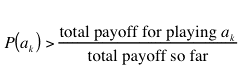
Figure 1. Final heuristics of all agents in example experiment for all learning frequencies. The red squares denote the mean heuristic for the final heuristics of this run

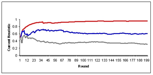
Figure 2. Development of the heuristics of three selected agents during a simulation run where the agents adapt their heuristic in every round

A first result of our simulations is the correlation between inertia in learning, the emerging specialisation, and route commitment.

Sum of Reward and Adaptation Rate

4.11

The question remains, whether a higher commitment to one route and thus a higher specialisation in the route choice contributes to all agents getting higher rewards. Table 2 shows the sum of rewards and the distribution of drivers between the two routes, while figure 3 depicts the distribution of drivers between both routes.

4.12

The highest average sum of reward - an indirect measure of the averaged driving time of all drivers - can be found in the experiment in which the inertia is small and the specialisation, high. There, also the standard deviation is quite low: there is no significant difference in the overall driving time. Experiments over a very long number of rounds show that all configurations result in a system with route commitment. However, the number of 200 route selection games was given by the real experimental setup.

Table 2: Sum of Reward averaged over all experiments and all agents and average distribution of drivers between the two routes (5 different scenarios)
Adaptation frequency	Sum of reward	Average number of drivers on main route (last 100 rounds)	Average number of drivers on secondary route (last 100 rounds)
1	1784 ± 69	12.4 ± 1.7	5.6 ± 1.7
5	1824 ± 95	12.2 ± 1.5	5.8 ± 1.5
10	1810 ± 81	12.2 ± 1.5	5.8 ± 1.5
20	1691 ± 153	12.7 ± 1.6	5.3 ± 1.6
50	1641 ± 130	13.3 ± 1.7	4.7 ± 1.7

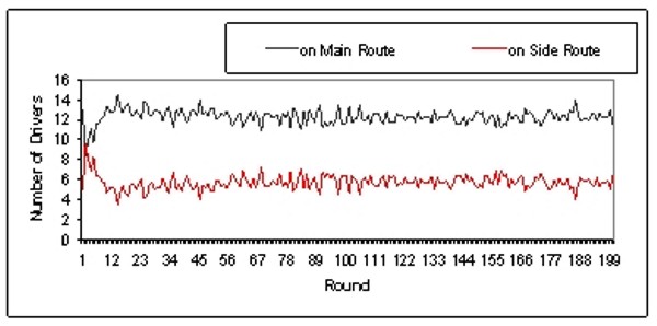
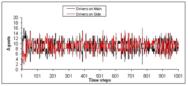
Figure 3. Development of the distribution of drivers in the Main and Side routes (Learning Frequency = 5, Initial Heuristic = 0.5)

Results for 900 Agents

4.13

Finally, we briefly discuss two extensions to what regards the standard settings we borrowed from the SURVIVE project (Selten et al. 2003). First, we show how the above results can be compared with the situation in which we simulate 900 agents. This extrapolates the capacity of laboratory experiments (at that time limited to 18 subjects), but is nevertheless an interesting anticipation. When N is set to 900, and agents learn with probability 0.2 at each period, the results are closer to the equilibrium point than in the case in which N is 18: the final heuristics agents associate with the main route is 0.668 (standard deviation equal to 0.323).

4.14

Since we have too many drivers to depict their individual performances, we have decided to have them classified in five categories according to their final heuristic learnt: side route drivers (0 ≤ final heuristic < 0.2), drivers with side route tendency (0.2 ≤ final heuristic < 0.4), random drivers (0.4 ≤ final heuristic < 0.6), drivers with main route tendency (0.6 ≤ final heuristic < 0.8), and main route drivers (0.8 ≤ final heuristic ≤ 1). The distribution after 400 simulation time steps can be seen in Figure 4 (again, average over 6 runs).

4.15

The second extension relates to performing a simulation in which initial heuristics are not the same for all agents anymore. Remember that up to here we have shown results for situations in which agents start with an initial heuristic equal to 0.5. Now we have changed this initial condition of route selection to allow each agent to have different initial heuristics, thus modelling drivers' individuality. These initial heuristics can now be anything between 0 and 1 (drawn from a normal distribution of probability). This simulation is depicted in Figure 5.

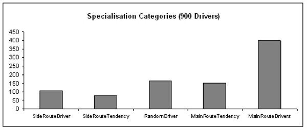
Figure 4. Number of drivers in each of the five categories; results regard scenario in which the learning takes place about every 5 rounds

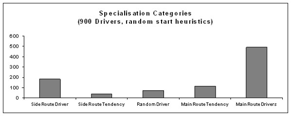
Figure 5. Number of drivers in each of the five categories; the learning takes place about every 5 rounds; initial heuristic to select main and side routes are equally distributed between 0 and 1

4.16

Comparing figure 4 and figure 5, we see that, from the former to the latter, the number of side route and main route drivers increases, while the number of agents in the three other categories decrease. Such increased specialisation is due to the adaptation process; only the drivers own experiences determine their adaptation to a scenario in which the initial heuristic is no longer equal for both routes.

Second Scenario: Reaction to Traffic Forecast

Description

5.1

The situation we focus on here is very similar to the one described in the previous section, however, now the decision process consists of two phases of decision-making. First, drivers make their initial route selection and inform the traffic control centre about their decisions. This is a metaphor we need in order to generate the forecast. One can assume that drivers give this information in exchange for reliable information regarding traffic forecast. Alternatively, one can think about gaining this information from detectors installed in both routes.

5.2

Based on the information collected, drivers receive a traffic forecast in the form of travel time for that particular route. Then, they have a second chance to actually take their first choice or change it. Finally the actual driving is carried out. The experiences drivers make in their actual driving influences both, their future selections of routes and their future reactions to traffic forecasts. This general idea is illustrated in Figure 8 in the appendix.

5.3

For the generation of forecast information and computation of actual travel times in form of rewards, we again use the formula given in Equation 3. For the generation of the drivers' first route decision, we also adopted the decision model described (first scenario). As in the most simple decision model for agents, it is based on a bias for choosing a certain route combined with a reinforcement learning scheme for its adaptation. After the final choice of the route and the reception of actual feedback, this tendency can be updated according to the experiences a driver has made. Again, the updating of heuristic is executed not in every time step, but approximately every fifth round on average (probability of 0.2 in every round).

5.4

Remember that, the more a driver selects a route, the more feedback information he gets from this route. However, route selection is not only based on this heuristic but also on driver's reaction on the forecasted reward. Moreover, the better his first choice is, the lesser he may need to reconsider his first decision. The consequence is that the success of this reinforcement scheme is interconnected with the way the driver reacts to the information about the situation after his first choice.

5.5

Similarly to the adaptation of the route selection heuristic, the reconsideration of the route choice (second decision) can also be based just on the experiences the driver has made in the previous rounds. To evaluate the forecasted reward, the driver needs some knowledge about the reward that is possible in the particular scenario (we call this a reference value). If the forecasted reward is less than the one he believes that it is good or realistic, then the driver makes a second selection of route. This means that there are three new aspects in comparison with the scenario in the previous subsection:

1. Generation of the reference value: The driver learns the reward that is possible in this scenario by taking into account the route length and the route selection behaviour of the other agents. The simplest form is to use a mean value of all previous feedback; alternatives are described in the last section.
2. Evaluation of the reference value: It might not be realistic that the previous successes that determined the reference value can be observed by the driver again. Therefore we introduced a tolerance. The extent of this tolerance determines how the drivers evaluate the reference value.
3. Reconsideration: There are different possibilities for reconsidering the first route decision. The obvious one might be that the driver simply selects the other route. This might lead to severe perturbations in scenarios with low tolerance values, even if the first route choice was not so bad due to the reward function that treats the two routes so unequally. Thus we decided to use another form of reconsideration: the driver ignores his first decision and randomly selects a route with equal probability.

Results and discussion for the Scenario with Forecast

5.6

We have first examined the effects of different shares of drivers who are unaware of or do not consider the information about the reward and thus always keep their first choice. Henceforth we write "ignorant" when referring to a driver who is unaware of the forecasted information.

5.7

We now present the results of different values of tolerance thresholds. Every simulation runs over 1000 time-steps representing 500 rounds: the odd and even time steps represent the first and the actual route decision respectively.

5.8

We have examined five situations with different shares of drivers reconsidering their first route choice: All drivers react on traffic forecast (Share of Ignorant = 0); 1/4, 1/2, and 3/4 of the drivers are ignorant. For sake of comparison, we use the experiments reported in the previous section (no driver receives or reacts to forecast).

Figure 6. Example of highly ineffective distribution of drivers on the two routes

5.9

Obviously - as illustrated in figure 6 - when all drivers react to the same forecasted information, a highly ineffective situation (from the point of view of the whole system) occurs. The pattern shown there resembles a random route choice behaviour. After some time, the distribution of drivers on the two routes happens exclusively based on the reconsideration of route decision based on the (in general very low) expected reward. As the reconsideration is based on a decision between the two routes according to equal probabilities, the learnt heuristics has no influence at all.

5.10

As described before (Section 4), the model without the reconsideration of route choice leads to the equilibrium. However, the more interesting situations happen between those extremes. Figure 7 shows the development of the expected reward over all drivers for different shares of ignorants. Each curve depicts the average value of rewards all drivers have received from their actual driving in all previous rounds. Thus it can be seen as a measure for the overall success of the drivers (remember, the reward in the balanced situation equals 10). On the other side, if the forecasted reward is less than this expected value, then the driver reconsiders his first choice.

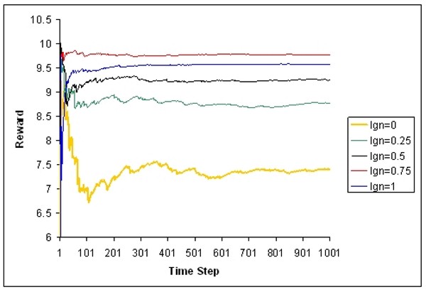
Figure 7. Development of the average expected reward in five example runs with different shares of drivers who react to traffic forecast

Table 3: Mean final heuristics of all drivers in five example runs with different shares of ignorant drivers
Share of ignorants	0	0.25	0.5	0.75	1
Final heuristics	1.06	0.80	0.67	0.67	0.68

5.11

In Table 3, the final heuristics averaged over five example runs are given. Notice that since the reward can be negative (as explained in Section 3), the final heuristic may look odd, with agents putting a probability higher than 1 on selecting the main route.

5.12

These results indicate that the reinforcement mechanism leading to route specialisation seems to make less sense when all drivers react in the same way to the same information. Considering these results, one can say that the best situation happens when there are 50-75% of drivers ignoring the traffic forecast. This is quite surprising, but may be a consequence of the sharp criteria - i.e. zero tolerance - for reconsidering the first route choice. The problem with the sharp criteria is that drivers always want to obtain the same reward they got in the previous rounds. If the forecasted reward is just a little bit lower than the average, the driver takes a new route decision. This means that even a few drivers on the wrong route could destroy the stability of the system if they make a decision which deviates from equilibrium. In other words, the system does not have any tolerance concerning a non-equilibrium configuration.

5.13

Therefore we also examined configurations in which drivers tolerate lower rewards. So far we have made experiments with tolerance levels of 1, 3, and 5. For example, if the expected reward is 10 and the driver receives a forecasted reward equal to 7, if the tolerance of this driver is 3, he accepts the reward and keeps its first route decision. However, if the tolerance level were 1, he would reconsider his decision..

Table 4: Drivers on main and on side routes (left); final heuristic (mean ± standard deviation) and mean expected reward (right): tolerances 1, 3, and 5, and share of ignorants 0, 0.25, 0.5, and 0.75
tolerance 1		share of	tolerance 1
drivers main	drivers side	ignorants	final heuristic	expected reward
9.11	8.84	0	1.06 ± 0.02	7.40
10.41	7.54	0.25	0.80 ± 0.10	8.78
11.33	6.61	0.5	0.67 ± 0.32	9.25
11.84	6.10	0.75	0.67 ± 0.32	9.77
12.25	5.70	1	0.68 ± 0.42	9.58
tolerance 3		share of	tolerance 3
drivers main	drivers side	ignorants	final heuristic	expected reward
11.49	6.45	0	0.73 ± 0.30	8.92
11.48	6.47	0.25	0.70 ± 0.30	9.29
11.84	6.11	0.5	0.68 ± 0.28	9.71
12.01	5.93	0.75	0.67 ± 0.33	9.61
tolerance 5		share of	tolerance 5
drivers main	drivers side	ignorants	final heuristic	Expected reward
12.34	5.61	0	0.68 ± 0.31	9.23
12.32	5.63	0.25	0.67 ± 0.29	9.29
11.94	6.01	0.5	0.68 ± 0.25	9.83
12.11	5.83	0.75	0.67 ± 0.28	9.27

5.14

To summarise, the most stable case occurs when the share of ignorants is 0.5 and the tolerance is high (5). Here, also the reward is the best one. This can be explained by the combination of high tolerance and a relatively high number of drivers receiving valuable information. If we reduce this share to, say, 0.25, then 75% of drivers would sometimes act randomly, thus adding perturbation to the system. Moreover, we noticed a correlation between a small inertia for adapting a heuristic, the resulting specialisation, and the overall benefit for the participants.

Conclusions and future work

6.1

Traffic systems are real-world systems that work without explicit communication, but with emergent co-ordination and more or less explicit social laws. Our long-term work focuses on commuting scenarios in which drivers have to make decisions, which on their turn alter the traffic condition. This paper continues on this track, by presenting simulations with agents that not only learn about which route to select, but also implicitly learn the "usual" route selections of the other road users. This has been mainly motivated by the results achieved in the SURVIVE project (Selten et al 2003). Therefore we avoid here the simulation of scenarios based on microscopic models and/or based on computation of other measurements like density of vehicles. These were tackled elsewhere (Klügl and Bazzan 2003).

6.2

Although the scenario is simple, it is possible to compare the results of this simulation to real experimental data. In both, experimental data and in our simulations, an analogous form of specialisation or route stability is observable.

6.3

Next, we want to extend the form of adaptation to consider more information, especially of social nature. This will lead to increasingly complex models that capture more and more details of the drivers' decision-making. Thus we hope to come with a model that incorporates social decision-making with explicit reasoning about inter-depending actions.

6.4

One may notice some critical points in the scenarios presented that lead to some interesting extensions. For instance, the route decision in our model is based on each driver's individual probability for the main route. This heuristic is a very condensed aggregation of all the experiences the driver makes during his route selection. By adapting to it, the driver learns about the length of the route and the usual density on that route. In our simulation experiments we used this simple model for the decisions of the driver and yet acquired results which compare to the real data (lab experiments). However, in order to improve this model, we want to consider the following aspects: social learning, experimental phases and inertia, and forecast.

Social Learning

6.5

The learning mechanism does not incorporate any explicit model of the environment (including other drivers at any aggregated level). There is no reasoning about the types of other participants or how they relate their experiences to their forthcoming route decisions. Individual decision rules such as "If X percent of the people that are now standing together with me in this jam, are taking the other route tomorrow, then I will be better off remaining on the same route" use explicit knowledge about other agents. This knowledge must be acquired. This requires an extension of the simple model by incorporating a kind of learning regarding what types of agents share the environment. But the scenario in which this learning happens is even more dynamical than the heuristic learning situation. The agents have to learn about the route itself and about the other agents' decision making. Moreover, this learning happens concurrently with the others. Such a scenario was partially tackled previously by us (Wahle et al. 2000). Although it is not clear that people really construct and use model about other drivers, its effects at least have to be tested. It is quite probable that model construction at least happens for driver categories (e.g. Porsche drivers versus drivers of small cars) or during actual driving with multiple contacts between drivers.

Experimental Phases and Inertia

6.6

We are assuming that all agents start to learn at the same point of time and adapt their heuristic in more or less the same periodicity during the complete game (although not synchronously). If we think about a commuter scenario in reality, there are at least three aspects that would require a modification of our simple model:

1. There is hardly any commuting situation where all drivers start learning about the route concurrently. In our scenario all agents start in the first round with no knowledge about basic costs or possible rewards. Moreover, also commuters that know the structure of the traffic system adapt if they are not satisfied anymore and see a chance that they may drive better in another route. Thus we need an individualisation in the frequency of adaptation.
2. Creation of an experimentation phase: from time to time a driver with an already converged heuristic starts to experiment. Thus he might drive on the other route, select routes randomly etc., and thus tries to gain new knowledge about the overall situation. Introduction of a discount factor for past actions: this would allow the model to put more weight on the more recent action selection.

Forecast

6.7

Concerning this issue, there are some possible extensions that may lead to more realistic behaviour, both at the driver level and at the overall traffic system level:

1. Quality of forecast: The "simulation" of the effects of the drivers' first decision is exact, as the same formula was used for computing the prognosis of reward. This assumption of exact forecast is not realistic. Thus an interesting extension could be to incorporate some form of noise in the form of uncertainty concerning the correctness of the forecast.
2. More detailed traffic models: Although the abstraction of travel time on different routes into a simple asymmetrical formula for rewards is the standard basis for game-theoretic treatments, there are other forms of microscopic traffic simulations that have proven to produce quite realistic overall system behaviour. An interesting modification of the model presented here, is the replacement of one or both steps of feedback generation by more realistic traffic simulations. A promising candidate is a microscopic traffic simulation model (Nagel-Schreckenberg 1992).
3. Sophisticated driver models: The way drivers decide whether to keep their first decision is rather inflexible and does not take into account other drivers reactions on the same information. If the driver could perceive some qualitative information about density (or number of drivers) on the route that he chose and the absolute numbers drivers that are in the system, then he might learn to estimate the other drivers decision-making (under the assumption that the other driver use the same algorithms for selecting their routes).
4. Different forms of traffic information: For the generation of the traffic forecast presented here, drivers have to submit their first choice to compute the forecast given to the drivers. Other kinds of information - with different associated costs - may be used to assess the future traffic situation for finally selecting one route.

Appendix: The Simulation Environment SeSAm

A.1

The models and experiments described in this paper were implemented and conducted using the multi-agent simulation environment SeSAm. The "Shell for Simulated Agent Systems" provides a generic environment for modelling and experimenting with agent-based simulations. Its development was specially focused on providing a tool for the fast and easy construction of complex models, as the main vision behind it was a tool for researchers without actual programming background (Klügl 2001).

A.2

In the following we want to present some important properties of SeSAm as a short introduction to the used simulation system. More information about SeSAm can obtained from http://www.simsesam.de.

SeSAmUML and Visual Agent Programming

A.3

SeSAm-Agents consist of a body that contains a set of state variables and a behaviour that is implemented in form of UML-like activity diagrams. Activities (the nodes of an activity graph) are seen as scripts that are initiated and terminated by firing rules. Based on this simple concept both, a specification language and a software environment for modelling and simulation were developed. The specification framework focuses on the representation of agent behaviour especially in relation to other agents, resources or the general environment (Oechslein et al., 2002). An example can be seen in Figure 8 where the specification framework is applied to the agent model with forecast reaction. It shows the different agent classes, their behaviour and interaction. Activity graphs are augmented with class diagrams for the agents´ internal structure. This is done for reasons of clarity as every part of the specified model should be visible at the same time.

A.4

In SeSAm there is basically a predefined distinction between agents (active entities), resources (passive entities) and the environment (global surrounding). Only in simple models no protocol-type specification of the agents interaction is necessary. In these cases, most interaction consists mainly of implicit coordination: One agent changes the environment more or less deliberatively. In our case this happens based on the route choice of the drivers which leads to interaction of drivers on the same route resulting in reduced driving time/reward. Any other agent may perceive the modified surroundings and adapts its behaviour according to it. More complex agent based models require a detailed specification of interaction sequences. Such a specification of an agent-based simulation model can be directly implemented using SeSAm, if the description provides sufficient details down to primitive actions and perception predicates. With every activity actions are associated which are executed when the agent is in this activity. Rules are responsible for termination and selection of activities. Actions of activities and conditions of rules can be composed from an extensive number of primitive building blocks. Figure 9 shows a screenshot of a part of the implementation of the specification shown above.

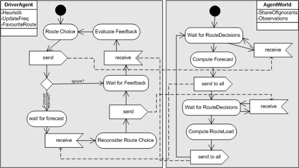
Figure 8. The specification of the behaviour of a driver agent in combination with the AgentWorld. A driver starts with selecting a route and announcing its choice to the world that computes a forecast for it. After having received the forecast the driver has the chance to reconsider its selection based on the information resulting in a final route choice. The world again acts as a traffic centre and returns travel information as a result of all route choices. Based on this information the driver evaluates its success adapting its route choice heuristic. These two combined graphs form the complete specification of the model with forecast information

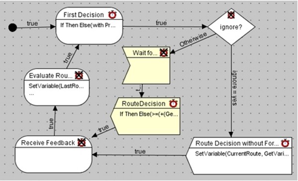
Figure 9. Screenshot from the SeSAm implementation of a driver agent according to the specification given in figure 8. The yellow nodes are the ones added when extending the scenario without forecast to the scenario with forecast

A.5

In addition to these normal activity nodes and rule arrows, also special forms of nodes like input or output nodes were introduce. These describe activities where the agent interacts with other agents and thus are marked for denoting this special purpose. Processing its activity graph initiates at the start node and terminates with the end node. The lifetime of an activity graph is over when the end node is selected. Activity graphs can be hierarchically organized in a way that a rule selects an activity graph instead of a simple activity. Additionally several activity graphs may determine the behaviour of an agent in parallel. The agent itself is terminated when one of its activity graphs ends. Thus the implementation of rather complex behaviour is possible that can even resemble the functionality of some reactive planning routines. As indicated in Figure 9, a user is able to design visually the behaviour of an agent. Analogous mechanisms are provided for specifying the static structures of an agent, an agent system or the environmental elements and their configuration. Thus a complete agent-based simulation model can be implemented visually without programming in a traditional programming language.

Modularization

A.6

Graphical modelling is built upon a set of predefined primitive elements – action primitive, perception primitive or operator primitive. They can be combined to function-calls visualized in form of a tree. Such an expression can be constructed every time when needed, or can be composed into user functions with arguments. They may represent more abstract building blocks or subroutines. Possible forms of combination are recursion, selection or composition. The primitive actions, perceptions and operators form the interface to the underlying programming language Java. For integrating such a Java method, it has to "declared" with additional information that describe its arguments, functionality, etc. This declaration is interpreted for the visual programming integration.

A.7

A set of attributes and user functions may be defined independently and grouped to a so called "feature" representing some notion of additional non-basic abilities that can be assigned to agents (or the environmental classes). They may be implemented visually by the modeller supporting modularization. Predefined features are for example spatial representation and functions that capture movement, or gene attributes with evolutionary operators. Another important issue is the question about the basic data types available for agents static structure and behaviour implementation. In addition to standard data types, like boolean, numeric, string values there are also composed data types like hash-tables or lists (with index-based access). Besides the built-in (or via features added) types a modeller can specify new types. They support sophisticated high-level agent structures and behaviors. There are two types of user types: enumerations and compositions. The range of first consists of a collection of symbols defined by the modeller for denoting aspects of the model, for example "main route" and "side route" as ranges for variable values. The second form of user defined data types is composition where an arbitrary number of attributes with other data types (also user defined ones) may be aggregated. Other important add-ons are interfaces to JDBC databases, like mySQL or the possibility to import ontologies (Protegé projects) and comfortable refactoring functionality. Thus SeSAm is also useful for large input data and complex data structures for simulation.

Simulation and Experimentation Support

A.8

All information about and parts of a simulation model – from agent structure and behaviour to relevant features and ready-to-run simulation run specification – are stored into a human-readable XML file based on a XML schema. Based on this model data format we developed a converter for a printable html visualization of a complete model.

A.9

Support for simulation cannot end when the model is implemented completely. Testing and executing experiments are also very demanding and effortful tasks. As there are freely configurable instruments for gathering data and scripting options for constructing simulation experiments on several computers concurrently, SeSAm is a highly valuable tool even for large scale agent based simulations.

Acknowledgements

Franziska Klügl and Ana L.C. Bazzan were partially supported by CNPq

References

BAZZAN, A. L. C., Wahle, J., Klügl, F. (1999) Agents In Traffic Modelling - from Reactive to Social Behaviour . Advances in Artificial Intelligence, Lecture Notes in Artificial Intelligence, Vol. 1701. Springer-Verlag, Berlin Heidelberg New York.

BEN-AKIVA,M., de Palma, A. and Kaysi, I. (1991) Dynamic network models and driver information systems. Transportation Research Part A 25(5): 251-266.

BURMEISTER, B., J. Doormann, and G. Matylis. (1997) Agent-oriented traffic simulation. Transactions of the Society for Computer Simulation International, 14(2), June 1997

CASTELFRANCHI, C. (1998) 'Modelling Social Action for AI Agents'. Artificial Intelligence, 103: 157 -182.

DE PALMA, A. (1998) Individual and Collective Decision Making: Applications to Travel Choice. Theoretical Foundations of Travel Choice Modelling, T. Gärling, T. Laitila, and K. Westin, (eds.), pp. 33-50, Elsevier, Oxford.

DIA, H., Purchase, H. (1999) Modelling the impacts of advanced traveller information systems using Intelligent Agents. Road and Transport Research, 8: 68-73.

FISCHER , K., Kuhn N., H.J.Müller, J.P.Müller and M. Pischel (1995) Sophisticated and Distributed: The Transportation Domain. In. Proc. of European Workshop on Modelling Autonomous Agents (MAAMAW 1993), LNAI 975, Springer.

HARLEY, C. B. (1981) Learning the Evolutionary Stable Strategy. Journal of Theoretical Biology, 89: 611-631.

KLÜGL, F.: Multi-Agent Simulation – Concepts, Tools, Application, Addison Wesley, Munich, (in German), 2001.

KLÜGL, F. and Bazzan, A. L. C. (2002) Simulation of adaptive agents: learning heuristics for route choice in a commuter scenario. Proc. of the First Int. Joing Conf. on Autonomous Agents and Multi-agent Systems (AAMAS 2002). ACM Press, 217-218

KLÜGL, F. and Bazzan, A. L. C. (2003) Selection of Information Types Based on Personal Utility – a Testbed for Traffic Information Markets. Proc. of the Second Int. Joing Conf. on Autonomous Agents and Multi-agent Systems (AAMAS 2003). ACM Press, 377-384.

MACY, M. W. and Andreas Flache (2002). Learning dynamics in social dilemmas. PNAS 99: 7229-7236.

MAYNARD-SMITH, J., Price, G. R. (1973) The logic of animal conflict. Nature, 246: 15-18,.

NAGEL, K. and M. Schreckenberg (1992). A cellular automaton model for freeway traffic. J. Phys. I France 2, 2221.

OECHSLEIN, C., Klügl, F., Herrler, R. and F. Puppe (2002). UML for Behavior-Oriented Multi-Agent Simulations. In: Dunin-Keplicz, B., Nawarecki, E.: From Theory to Practice in Multi-Agent Systems, CEEMAS 2001 Cracow, Poland, September 26-29, 2001, (= LNCS 2296), Springer, Heidelberg, pp. 217ff

OSSOWSKI, S. (1999) Co-ordination in artificial agent societies, social structures and its implications for autonomous problem-solving agents. (LNAI, Vol. 1535). Springer, Berlin.

ROSSETTI, R.J.F., Bampi, S., Liu, R., Van Vliet, D., Cybis, H.B.B. (2000) An Agent-Based framework for the assessment of drivers' decision-making. Proc. of the 3rd Annual IEEE Conference on Intelligent Transportation Systems, Oct. 2000 Dearborn, MI, Proceedings, Piscataway: IEEE, p.387-392.

ROTH, A. E. & Erev, I. (1995) Learning in extensive form games: experimental data and simple dynamic models in the intermediate term. Games Econ. Behav. 8, 164-212

SELTEN, R., Schreckenberg, M., Pitz, T., Chmura, T. and Wahle, J. (2003) Experimental Investigation of Day-to-Day Route Choice-Behaviour. R. Selten and M. Schreckenberg (eds.) Human Behavior and Traffic Networks, Springer (to appear).

SRINIVASAN, K. K. and Mahmassani, H. S. (2003) Analyzing heterogeneity and unobserved structural effects in route-switching behavior under ATIS: a dynamic kernel logit formulation. Transportation Research Part B 37(9): 793-814.

WAHLE, J., Bazzan, A. L. C., Klügl, F., Schreckenberg, M. (2000) Decision Dynamics in a Traffic Scenario. Physica A, 287 (3-4): 669 - 681.

WAHLE, J., Bazzan, A. L. C., Klügl, F., Schreckenberg, M. (2002) The Impact of Real Time Information in a Two Route Scenario using Agent Based Simulation. Transportation Research Part C: Emerging Technologies 10(5-6): 73 – 91.

Return to Contents of this issue

© Copyright Journal of Artificial Societies and Social Simulation, [2003]