Brian Sallans, Alexander Pfister, Alexandros Karatzoglou and Georg Dorffner (2003)
Simulation and Validation of an Integrated Markets Model
Journal of Artificial Societies and Social Simulation
vol. 6, no. 4
To cite articles published in the Journal of Artificial Societies and Social Simulation, please reference the above information and include paragraph numbers if necessary
<https://www.jasss.org/6/4/2.html>
Received: 14-Feb-2003 Accepted: 14-May-2003 Published: 31-Oct-2003
 Abstract
 |
| Feature | Description |
| Assets | 1 if assets increased in the previous iteration, 0 otherwise |
| Share Price | 1 if share price increased in the previous iteration, 0 otherwise |
| Mean Price | 1 if product price is greater than mean price of competitors, 0 otherwise |
| Cluster Center 1 | A bit-vector that encodes the position of cluster center 1 |
| ... | ... |
| Cluster Center N | A bit-vector that encodes the position of cluster center N |
| Action | Description |
| Random Action | Take a random action from one of the actions below, drawn from a uniform distribution |
| Do Nothing | Take no actions in this iteration. |
| Increase Price | Increase the product price by 1. |
| Decrease Price | Decrease the product price by 1. |
| Move down | Move product in negative Y direction. |
| Move up | Move product in positive Y direction. |
| Move left | Move product in negative X direction. |
| Move right | Move product in positive X direction. |
| Move Towards Center 1 | Move the product features towards cluster center 1. |
| ... | ... |
| Move Towards Center N | Move the product features towards cluseter center N. |
![$\displaystyle Q^\pi(\vec{s},a) = E\left[ \sum_{\tau=t}^{\infty} \gamma^{\tau-t}r_{\tau} \vert \vec{s}_t=\vec{s}, a_t=a \right]_\pi$](2/img35.png) |
(4) |
where
![]() is the wealth at time
is the wealth at time ![]() and
and ![]() the number of stocks
of the risky asset hold at time
the number of stocks
of the risky asset hold at time ![]() .
As in (Brock and Hommes, 1998) , (Levy and Levy, 1996) , (Chiarella and He, 2001) , and (Chiarella and He, 2002)
the demand functions of the following models are derived from a Walrasian scenario.
This means that each agent is viewed as a price taker
(see (Brock and Hommes, 1997) and (Grossman, 1989) )
.
As in (Brock and Hommes, 1998) , (Levy and Levy, 1996) , (Chiarella and He, 2001) , and (Chiarella and He, 2002)
the demand functions of the following models are derived from a Walrasian scenario.
This means that each agent is viewed as a price taker
(see (Brock and Hommes, 1997) and (Grossman, 1989) )
| Price per share of the risky asset at time |
|
| Dividend at time |
|
| Risk free rate | |
| Total number of shares of the risky asset | |
| Total Number of investors | |
| Number of shares investor |
|
| Wealth of investor |
|
| Risk aversion of investor |
|
| Parameter | Description | Range | Value | Reference |
|
|
strength of profitability reinforcement | |
0.47 | Eq.(2) |
|
|
strength of stock price reinforcement | |
0.53 | Eq.(2) |
|
|
Number of cluster centers |
|
2 | section 3.1.1 |
|
|
product update rate |
|
0.03 | Eq.(1) |
|
|
reinforcement learning discount factor | |
0.83 | Eq.(3) |
|
|
History window length for firms |
|
3 | section 3.1.1 |
|
|
Proportion of fundamentalists | |
0.57 | section 4 |
|
|
Proportion of chartists | |
0.43 | section 4 |
|
|
Fundamentalist price update rate | |
0.18 | Eq.(22) |
|
|
Chartist price update rate | |
0.36 | Eq.(23) |
|
|
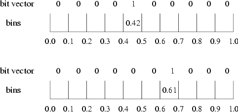
Number of bins |
|
10 | figure 3 |
|
|
product update frequency |
|
8 | section 2 |
|
|
base salary |
|
0 | Eq.(2) |
|
|
reinforcement learning rate |
|
0.1 | Eq.(8) |
|
|
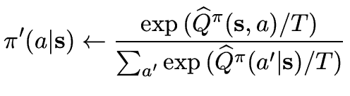
reinforcement learning temperature | |
|
Eq.(9) |
|
|
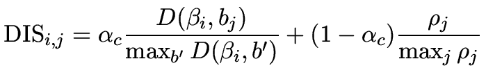
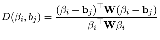
Consumer feature/price tradeoff | |
0.5 | Eq.(10) |
|
|
Maximum dissatisfaction for consumer |
|
0.8 | Eq.(12) |
|
|
inverse fair dividend yield |
|
50 | Eq.(21) |
 |
(25) |
 |
(26) |
 |
 |
 |
(27) |
 |
 |
 |
 |
2
We will drop the firm index ![]() in this section for
clarity. The same reinforcement learning algorithm is used for each firm, with
the same parameter settings. Each firm learns its own value function from
experience.
in this section for
clarity. The same reinforcement learning algorithm is used for each firm, with
the same parameter settings. Each firm learns its own value function from
experience.
3
Note that at time ![]() price
price
![]() and dividend
and dividend ![]() are not included in the information set
are not included in the information set ![]()
4
The risk free
interest rate ![]() was set to 1.5%. Because of the fact
that holding the stock is riskier, the fair dividend yield should
be above the risk free rate.
was set to 1.5%. Because of the fact
that holding the stock is riskier, the fair dividend yield should
be above the risk free rate.
5
Note that for chartists
![]() for computing an average price change.
for computing an average price change.
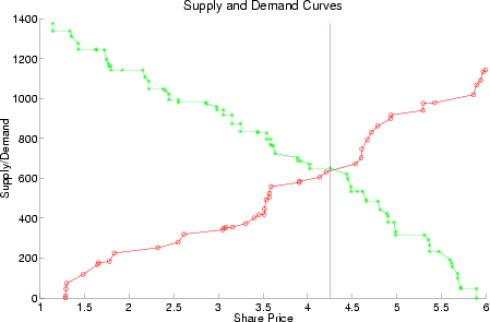
6 A limit order is an instruction stating the maximum price the buyer is willing to pay when buying shares (a limit buy order), or the minimum the seller will accept when selling (a limit sell order).
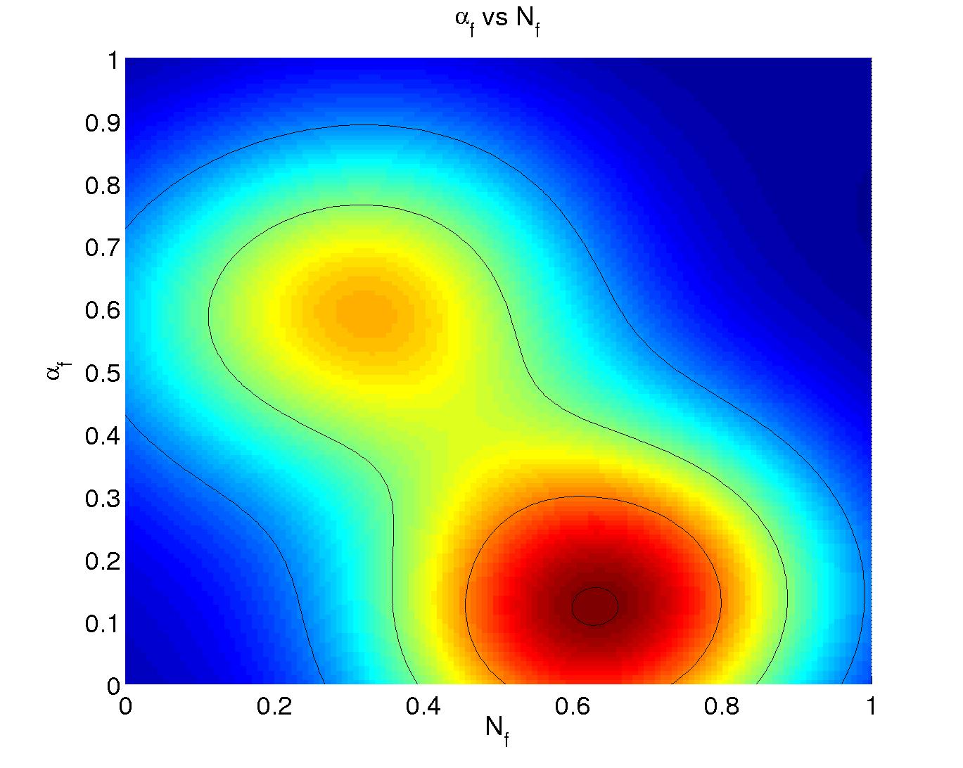
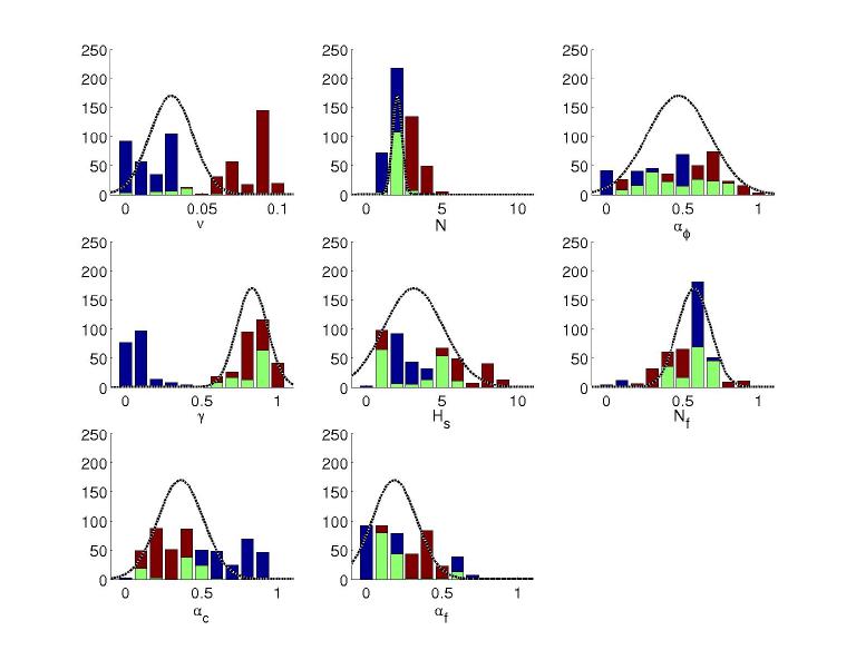
7 The density plots were generated using the kernel density estimator for Matlab provided by C.C. Beardah at http://science.ntu.ac.uk/msor/ccb/densest.html (Beardah and Baxter, 1996).
8 Significance was measured in the following way: First, the sequence of parameter values was subsampled such that autocorrelations were insignificant. Given this independent sample, the correlations between parameters could be measured, and significance levels found.
 Return to Contents of this issue
© Copyright Journal of Artificial Societies and Social Simulation, [2003]
![$\displaystyle R_t = E\left[ \sum_{\tau=t}^{\infty} \gamma^{\tau-t}r_{\tau} \right]_{\pi}$](2/img27.png)
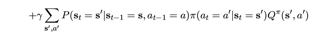
![$\displaystyle E\left[ \sum_{\tau={t-1}}^{\infty} \gamma^{\tau-t+1}r_{\tau} \vert \vec{s}_{t-1}=\vec{s}, a_{t-1}=a \right]_\pi$](2/img44.png)
![$\displaystyle E\left[ r_{t-1} \vert \vec{s}_{t-1}=\vec{s},a_{t-1}=a\right]_\pi ...
...fty} \gamma^{\tau-t}r_{\tau} \vert \vec{s}_{t-1}=\vec{s}, a_{t-1}=a \right]_\pi$](2/img45.png)

![$\displaystyle \mathop {\max }\limits_{q_{m,t} } \left\{ {E_{m,t} \left[ {W_{m,t...
...\right] - \frac{{\zeta _m }} {2}V_{m,t} \left[ {W_{m,t + 1} } \right]} \right\}$](2/img88.png)
![$\displaystyle q_{m,t} = \frac{{E_{m,t} \left[ {p_{t + 1} + d_{t + 1} } \right] ...
... \kappa} \right)}} {{\zeta _m V_{m,t} \left[ {p_{t + 1} + d_{t + 1} } \right]}}$](2/img89.png)
![$\displaystyle E_{m,t} \left[ {d_{t + 1} } \right] = \frac{1} {{h_m }}\sum\limits_{j = 1}^{h_m} {d_{t - j} }$](2/img102.png)

![$\displaystyle E_{m,t} \left[ {p_{t + 1} } \right] = p_{t - 1} + \alpha_n \left( {\frac{{p_{t - 1} - p_{t - h_m } }} {{h_m - 1}}} \right)$](2/img111.png)
![$\displaystyle E[f(\vec{x})]_{P(\vec{x})} \approx \frac{1}{N} \sum_{i=1}^N f(\vec{x}_i)$](2/img131.png)