© Copyright JASSS

  JASSS logo ----

H. Fort (2003)

Cooperation with random interactions and without memory or "tags"

Journal of Artificial Societies and Social Simulation vol. 6, no. 2
<https://www.jasss.org/6/2/4.html>

To cite articles published in the Journal of Artificial Societies and Social Simulation, please reference the above information and include paragraph numbers if necessary

Received: 19/12/2002      Accepted: 16-Feb-2003      Published: 31-Mar-2003
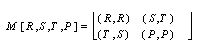

* Abstract

The self-organization into cooperative regimes of a system of "selfish" agents playing the pairwise Prisoner's Dilemma game (PDG) is analyzed using a simple agent-based model. At each time step t, the agents divide into those who cooperate (C) and those who defect (D). The agents have no memory and use strategies not based on direct reciprocity nor 'tags'. Only one dynamical variable is assigned to each agent, namely his income at time t, δ C(t), obtained by playing the PDG with a partner chosen at random. A simple adapting strategy for the behavior of the agents (C or D) is shown to give rise, for a wide variety of PD payoff matrices, to a cooperative regime resistant to 'always D' strategy.

Keywords:
Complex Adaptive Agents; Cooperation; Evolutionary Model; Game Theory; Prisoner's Dilemma

* Introduction

1.1
The Prisoner's Dilemma (PD) embodies the central ingredients of the emergence of cooperation in societies of "selfish" individuals (individuals which pursue exclusively their own self-benefit) in a very simple and intuitive way. There are two players, each confronting two choices: cooperate (C) or defect (D) and each makes its choice without knowing what the other will do. Independently of what the other player does, defection D yields a higher payoff than cooperation and is the dominant strategy. The dilemma is that if both defect, both do worse than if both had cooperated. That is, there are four possible outcomes for the interaction of agent Ai with agent Aj: (1) they can both cooperate ( [C,C] ), (2) both defect ( [D,D] ), (3) Ai cooperates and Aj defects ( [C,D] ) and (4) AI defects and Aj cooperates ([D,C]). Depending on the situation (1) - (4), the agent AI (Aj) gets respectively: the "reward" R (R), the "punishment" P (P), the "sucker's payoff" S (the "temptation to defect" T) or T (S), i.e. the payoff matrix M[R,S,T,P] is

1.2
The payoff matrix gives the payoffs for row behavior when confronting with column behavior.

1.3
This approach has been used extensively to examine the basis of the cooperation problem in a wide variety of contexts: see for instance Axelrod (1984, 1997), Chapter 3 of Axelrod and Cohen (1999), and for a recent review, Hoffman (2000).

In order to have a dilemma it is required that:

T > R > P > S. (1)

In case one wants that universal cooperation be Pareto optimal, the additional required condition is:

2R > S + T. (2)

1.4
The emergence of cooperation in iterated PD games is generally assumed to require repeated play and strategies such as Tit for Tat (TFT) (Axelrod 1997, 1984), involving memory of previous interactions or features ("tags") permitting cooperators and defectors to distinguish one another.

1.5
Here I consider the simplest version of a model of selfish agents, possessing neither memory[1] nor tags, in which at each time step pairs of agents are selected to play the PD game. At time t the behavior of any agent is one of two alternatives: cooperate (C) or defect (D). All the agents use the same measure of success to evaluate if they did well or badly in the game which implies comparison of the income they received with an estimate of expected utilities and the arithmetic mean of payoffs Mav ≡ (R+S+T+P) /4. Next, they update their behavior (C or D) in consonance, that is a player keeps his behavior if he did well and changes it if he did badly. It turns out that depending on the relation between R and Mav and between P and Mav, after a transient, the system self-organizes into two different equilibrium states characterized by their average probability of cooperation peq (or equivalently the fraction of C-agents fC): peq = 0.5 and peq = 0.0. The canonical payoff matrix M[3,0,5,1] ( R=3, S=0, T=5, and P=1) is used to illustrate how the system works. The analysis is also extended to other payoff matrices.

1.6
We will see that the proposed mechanism for adapting the behavior of agents can be translated in terms of the more traditional mechanism in which agents learn by imitating the behavior of those successful partners which get a higher score.

* A Mechanism to produce Cooperative Equilibrium States

2.1
I consider the simplest version in which the pairs of players are chosen randomly instead of being restricted to some neighborhood. The suitability of the random treatment depends on several features such as the population size, the degree of connectivity, etc. For instance, if the agents display high mobility or they can interact at a distance (for example electronic transactions and so on) the random version seems appropriate. In this work the population of agents, N, will be of the order N=1000.

2.2
The mechanism which gives rise to cooperative regimes between selfish agents is based on comparison of their utilities with an estimate. An arbitrary agent say number k, given the average probability of cooperation pfC , can estimate his utilities as the income δCk(R,S,T,P) he makes by playing with an "agent" which cooperate with probability p :

(3)

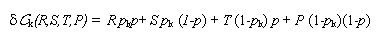
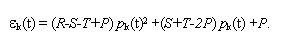
where the variable pk takes only two values: 1 if k is a C-agent and 0 if k is a D-agent. It turns out that, in general, the value of p is not known by the agents. Thus a simpler estimate of the expected utilities εk is obtained by substituting p in the above expression for the per-capita-income δ Ck (R,S,T,P) by his own probability of cooperation pk[2]. In other words, agent k makes the simplest possible extrapolation and assumes that the average probability of cooperation coincides with his pk; the estimate εk corresponds to the utilities he would made by playing with himself. That is,

(4)

2.3
From this equation, if the agent is C i.e. pk =1 then εk(t)=R while if pk =0 then εk(t)=P i.e.

(5)

2.4
The measure of success is as follows: if δC k (R,S,T,P) ≥ (<) max{ εk(R,S,T,P), Mav}[3] the agent assumes he is doing well and he keeps (inverts) his behavior C or D.

2.5
The initial state at t = 0 is taken as C and D chosen at random for each agent (we will see that the equilibrium states are independent of the initial configuration of probabilities of cooperation). From this state the system evolves by iteration during tf time steps using the following procedure:

  • Selection of players: At each time step t two agents AI and Aj, chosen at random, are selected to interact i.e. to play the PD game.
  • PD game: The player k gets a profit δC k(t) which is one of the four PD payoffs: R, S, T or P.
  • Assessment of success: Each of the two agent who have just interacted compare their income δC k(t) with his estimate εk(t) for expected utilities.
    If the agent assumes it is doing well (badly) and therefore his behavior (C or D) is adequate (inadequate).
  • Behavior update: If player k is doing well he keeps his behavior. On the other hand, if he is doing badly he changes his behavior from C to D or from D to C.

Remarks

  1. All the agents use the same universal behavior update rule (which does not evolve over time). However, the system is adaptive in the sense that the behaviors of the agents do evolve.
  2. The proposed strategy is similar to the one named 'Pavlov' by the mathematicians D. P. Kraines and V. Kraines (Kraines 1989). After experiencing a reward for mutual cooperation or getting away with unilateral defection, a Pavlov player repeats the former cooperative move. But after being punished for mutual defection or after getting the sucker's payoff for unilaterally cooperating, Pavlov inverts his behavior (switches to C or D respectively). In short, the Pavlov rule says to stick to the former move if it earned a high payoff (reward R or temptation T) but to switch if the last move brought a low return (punishment or sucker's payoff). However, the strategy based on the estimate covers a wider range of situations than Pavlov. In fact it coincides with Pavlov only when T and R are greater than Mav[4]. Further-more, for matrices which do not fulfill the PD condition (1), that might be used to simulate minorities of "abnormal" individuals[5], the outcomes can depart dramatically from Pavlov. In the next section some specific examples are discussed.
  3. Concerning comparison with TFT or other direct reciprocal strategies: note that the problem addressed is different from that of the evolution of cooperation. Here we do not have competition of different strategies. Thus the use of, for instance, TFT would imply a trivial result: all the agents start C and keep that behavior. Indeed, in the next section we will see that, the proposed strategy works to establish cooperative states even if at the very beginning there are no cooperative subjects.

* Results

3.1
For the canonical payoff matrix M[3,0,5,1] the system self-organizes, after a transient, in equilibrium states with peq = 0.5 (this equilibrium value can be easily computed analytically as will be shown later in this section). The measures are performed averaging over 1000 simulations.

3.2
In order to show that the initial fraction of C-agents fC0 only affects the transient regime (before equilibrium is reached) and has no effect on the final equilibrium state, Fig. 1 shows the average probability of cooperation <p> for different values of fC0 . In particular, note that even for fC0 = 0 the system evolve towards an equilibrium state with peq = 0.5, i.e. the existence of cooperative agents at the very beginning (t = 0) is not a necessary condition to reach this cooperative equilibrium state.

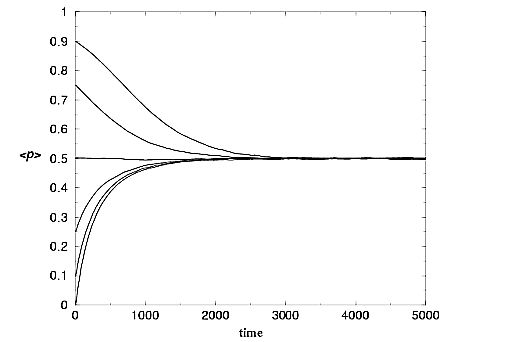
Figure 1. <p> vs. time, for the canonical payoff matrix. fC0 = 0, 0.1, 0.25, 0.75 and 0.9.

3.3
Depending on the payoff matrix the equilibrium asymptotic states can be of two types: cooperative (peq = 0.5) and of "all D" (peq = 0). Let us show this by a simple calculation. Note that the adapting rule implies that if δCk < ( max {εk, Mav} (remember that εk = R in the case of a C-agent and εk = P in the case of a D-agent) then the agent keeps his behavior and, on the contrary, if 
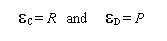
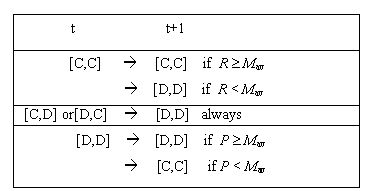
he inverts his behavior. In an encounter [C,C] both agents get δC = R which coincides with their estimate εC= R, hence they keep their behavior if and otherwise change their behavior to D if R < Mav. On the other hand, in an encounter [D,D] both agents get δC = P which coincides with their estimate εD= P, hence they keep their behavior if 
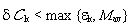
and otherwise change their behavior to C if P < Mav. Finally, In an encounter [C,D] the C-agent gets δCC = S and his estimate is εC = R and the D-agent gets δCD = T and his estimate is εCD= P. Hence, the C-agent would keep his behavior if S ≥ max {R, Mav}, but this cannot happen because S < R then he changes to D. The D-agent keeps his behavior because T = max {R,S,T,P} and then T ≥ max {P, Mav}. After the four kind of possible encounters the 2 interacting agents end with the same behavior (C or D). Table 1 summarizes the possible outcomes for payoff matrices satisfying the PD condition (1).

Table 1. Possible outcomes for the different PD game interactions.

3.4
Note that when RMav and P < Mav half of the transitions from time t to t+1 lead to C (those from [D,D] ) and the other half to D (those from [C,D] or [D,C]) producing an equilibrium state with peq = 0.5. These transitions are identical to Pavlov's transitions (see for instance Nowak, May and Sigmund 1995). On the other hand, when RMav or PMav the balance between transitions to C and D breaks down in favor of D producing an equilibrium state with peq = 0.0 (i.e. transitions different from Pavlov's transitioms). Equation (1) restricts the values that R and P can take for a given Mav: we have that R < 2Mav (R tends to 2Mav when T is slightly higher than R, and P and S infinitsimal) and P < 4/3Mav (P tends to 4/3 Mav when T and R are slightly higher than P and S infinitesimal) . Therefore, as is shown in Fig.2, we have two regions in the payoff space (R, P), the bottom-right square delimited by:

(6)

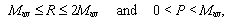
for which the proposed strategy produces cooperation (in gray), and the rest for which peq = 0.0 (in white).

Figure 2. Different region in the (R,P) plane: cooperative (gray) and non-cooperative (white).

3.5
The existence of PD games leading both to cooperative and non-cooperative equilibrium opens the interesting possibility of analyzing mixtures of agents using different payoff matrices giving rise to a continuous range of values for peq in the interval from 0.0 to 0.5 instead of only peq = 0.5. That is, when 100% of the agents use a payoff belonging to the gray (white) region we get peq = 0.5 (peq = 0.0), in the intermediate cases peq interpolates between these two values.

3.6
Additionally, in the case, previously mentioned, of minorities using payoff matrices not fulfilling the PD condition (1), new differences appear between this strategy and Pavlov. In particular we find a situation which is just the opposite situation we found before: the proposed strategy produces a cooperative state while Pavlov leads to peq = 0.0.

3.7
Let us see some illustrative examples. For instance, the canonical payoff matrix M[3,0,5,1] has Mav = 2.25 and thus if both players are C, both get δC ≡ R = 3 = max {3, 2.25 } and thus both remain C, while if both are D, they get δCP = 1 < 2.25 = max {1, 2.25 } and thus both change to C. Another example is provided by payoff matrix M[4,0,5,3] which has Mav = 3 and thus if both players are C, both get δ C R = 4 = max {4, 3} and thus both remain C, while if both are D, they get CP = 3 = max {3, 3} and thus both remain D. As a final example consider the payoff matrix M[0,3,4,5] which violates conditions (1) and (2). In this case, which implies no dilemma at all, one would bet that it leads to "all D" state - as in fact happens with Pavlov. However, the outcome is different for the proposed strategy because non reciprocal encounters ([C,D] or [D,C]) now lead to [C,C] instead of to [D,D], which in turn results in peq = 0.5 instead of peq = 0.0. In Table 2 the transitions from t to t+1 are summarized for payoff matrices M[3,0,5,1] and M[4,0,5,3]. We can see, from Table 2, that for payoff matrix M[3,0,5,1] half of the transitions from time t to time t+1 lead to [C,C] and the other half to [D,D] while for payoff matrix M[4,0,5,3] the transitions to [D,D] surpass those to [C,C] ( two third vs. one third). Therefore, it is evident that for payoff matrices M[3,0,5,1] and M[4,0,5,3] the system converge to equilibrium states with, respectively, equal proportion of C-agents and D-agents (peq=0.5) and all D-agents (peq=0.0). This can be checked easily by solving an algebraic equation for peq.

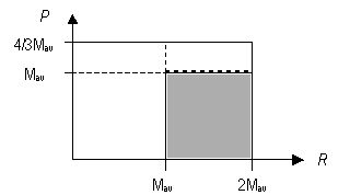
Table 2. Transitions for payoff matrices M[3,0,5,1], M[4,0,5,3] and M[0,3,4,5]

3.8
To obtain this equation note that, for a given average probability of cooperation p at time t, the probabilistic weights for the four possible kind of encounters are: p2, p(1-p), (1-p)p and (1-p)2. Hence, for payoff matrix M[3,0,5,1] the transitions from D to C are proportional to 2(1-p)2 and the transitions from C to D are proportional to 2p(1-p). For payoff matrix M[4,0,5,3] there are no transitions from D to C and the transition from C to D is proportional to 2p(1-p). Once equilibrium has been reached the transitions from C to D and from D to C must be equal and then the average probability of cooperation peq is obtained by equalizing both fluxes. That is, for M[3,0,5,1]

2(1-peq)2 = 2 peq(1-peq) (7)

one of its roots is peq=0.5 (the other root is peq=1); and for M[4,0,5,3] we have

0 = 2 peq(1-peq) (8)

one of its roots is peq=0.0 (the other root is peq=1).

3.9
Fig. 3 shows p as a function of time the both for M[3,0,5,1] and M[4,0,5,3].

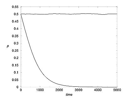
Figure 3. p vs. time, for payoff matrices M[3,0,5,1] with peq=0.5 and M[4,0,5,3] with peq=0.0.

3.10
The proposed mechanism can be analyzed from the more traditional point of view of Evolutionary Game Theory (Maynard Smith 1982, Weinbull 1995) in which agents learn from and copy the successful strategies of others. For instance, in the spatial games of Nowak and May (Nowak and May 1992) players are located on fixed positions on a spatial lattice. Each player plays only with other players in his neighborhood. After a round of play, the player changes strategy (learns) according to the rule "imitate the partner (which in these spatial games is a neighbor) who did best in the previous round." In this simple model each agent interacts with only one partner chosen at random. It is easy to realize hat the behavior update considered in this work is equivalent to introduce a modification in the learning rule: "imitate the partner who did best in the previous round if his income is no less than the average of possible payoffs Mav_ ." This modification is critical in order to reach a cooperative regime, otherwise there is no escape to the "all D" Nash equilibrium.

3.11
Moreover, the Nowak-May spatial game algorithm reaches cooperative states (peq > 0) for the case of a "weak dilemma" in which P = S = 0 or at most when P is significantly below R. In particular, in a spatial game in which each player interacts with his four nearest neighbors, I have checked for the case of the canonical payoff matrix, that the ordinary evolution rule leads to an all-D state while the modified rule produces a cooperative equilibrium state with peq = 0.5.

3.12
To end this section let us briefly analyze the per-capita-income δC [R,S,T, P](p) as a function of the average probability of cooperation p, which is obtained by replacing in equation (3) pk by p i.e.

(9)

3.13
As p in equilibrium is equal to 0.5 or 0 then we have two possibilities for δCeq [R, S,T, P] ≅ (δ C [R S T P](peq):

(10)

* Summary and Conclusion

4.1
I would like to remark the robustness of the combination of the measure of success + the behavior update rule to develop and sustain a cooperative regime. Specifically, a payoff matrix like the canonical one M[3,0,5,1] which, according to the traditional evolutionary adaptation rule of imitating the more successful players, would lead to an "all D" state, actually produces an equilibrium state with peq=0.5. Furthermore, we realized that the proposed mechanism in fact is equivalent to a more exigent requirement in order to imitate the behavior of successful players: "imitate those partners who did best in the previous round only if his income is no lees than the average of possible payoffs Mav".

4.2
We have seen that the proposed strategy comprises strategies of the kind of "win-stay, lose-shift" but is more general than this and it is able to cover a much wider range of situations depending on the payoff matrix. To be more specific, it seems more realistic to assume that different persons "use" different payoff matrices. This would give rise to richer situations leading to a peq which, in principle, could take a continuous range of values. Furthermore, this strategy, when extended to payoff matrices which imply no dilemma at all, produces outcomes which clearly, at least at first sight, defy our intuition. For instance, the case of payoff matrices with cooperative payoffs - reward R and the sucker's payoff S - smaller than the payoff for defection -the temptation T and the punishment P - for which the strategy manages to produce a cooperative equilibrium. The specific example of that is the payoff matrix M[0,3,4,5], with null reward!

4.3
In this work all the spatial correlation between agents were neglected. One virtue of this simplification is that it shows the model does not require that agents interact only with those within some geographical proximity in order to sustain cooperation. Playing with fixed neighbors is sometimes considered as an important ingredient to successfully maintain the cooperative regime (Cohen, Riolo and Axelrod 2001, Nowak and May 1992). The random selection of players also introduces a non-deterministic component in the algorithm which might be of importance depending on the context. Additionally, the equilibrium points can be obtained by simple algebra independently from the initial conditions. However, the quality of this approximation depends on the nature of the system one desires to model (people, cultures of bacteria, market of providers of different services or products, etc.).Therefore, in order to apply the model to situations in which the effect of geographic closeness cannot be neglected an interesting extensions of the model is to transform the entirely random PD game into a spatial PD game, in which individuals interact only (or mainly) with those within some geographical proximity (Fort 2002).

* Acknowledgements

I thank R. Axelrod, R. Donangelo and H. Gintis for valuable discussions and opinions. I thank M. Reisenberger for criticism of the manuscript.


* Notes

1 The players do not keep track of the game's history, perhaps, instead of 'no memory' it would be more precise to say that agents have only memory of the previous interaction or that they use no explicit long term memory.

2 One might consider more sophisticated agents which have "good" information (statistics, surveys, etc.) from which they can extract the average probability of cooperation in "real time" p(t) to get a better estimate of their expected utilities. However, the main results do not differ substantially from the ones obtained with these simpler agents.

3 max{A,B} stands for the maximum of A and B.

4 The choice of Mav as a reference point is quite arbitrary, indeed whether or not cooperation becomes a stable strategy depends on the fact that two payoffs are greater and the other two smaller than the reference point.

5 For instance "altruists", C-inclined independently of the costs, with payoff matrices with high values of S or "anti-social" individuals, for whom cooperation never pays, with very low values of R.


* References

AXELROD, R. (1984), The Evolution of Cooperation, Basic Books, New York.

AXELROD, R. (1997), The Complexity of Cooperation, Princeton University Press.

AXELROD, R. And COHEN M. (1999), Chapter 3 of Harnessing Complexity, The Free Press.

COHEN , M. D. ,RIOLO R. L. and AXELROD R. (2001), Rationality and Society 13: 5.

FORT, H. (2002) to be published elsewhere.

HOFFMANN, R. (2000), Journal of Artificial Societies and Social Simulation 3 (2). <https://www.jasss.org/3/2/forum/1.html>

KRAINES, D. P. and KRAINES V. 1989, Theory and Decision 26 (1989): 47.

MAYNARD SMITH, J. 1982, Evolution and the Theory of Games, Cambridge University Press.

NOWAK M. A. and MAY R 1992., Nature 359: 826.

NOWAK M. A., MAY R. and SIGMUND K. 1995, Scientific American, June 1995: 76.

WEINBULL, J. W. 1995, Evolutionary Game Theory, MIT Press.

----

ButtonReturn to Contents of this issue

© Copyright Journal of Artificial Societies and Social Simulation, [2003]