
D.W. Pearson and M-R. Boudarel (2001)
Pair Interactions : Real and Perceived Attitudes
Journal of Artificial Societies and Social Simulation
vol. 4, no. 4
To cite articles published in the Journal of Artificial Societies and Social Simulation, please reference the above information and include paragraph numbers if necessary
<https://www.jasss.org/4/4/4.html>
Received: 29-Mar-01
Accepted: 30-Sep-01
Published: 31-Oct-01
 Abstract
![]() Introduction
Introduction
Development of a Mathematical Model
|
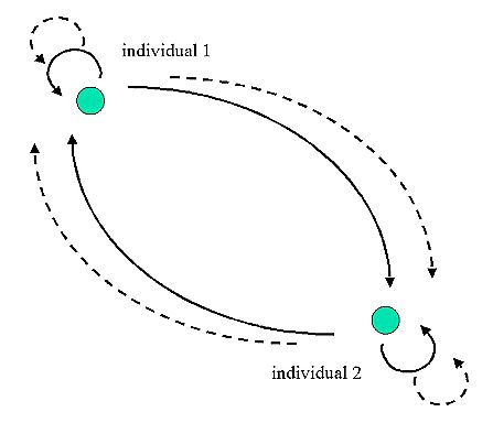
| Figure 1: Pair interaction of two individuals |

 . Notice that we assume only local transitional probabilities, i.e. we only allow a transition from n to n-1 or n+1 and not to n-2, n+2 etc. We thus avoid collective attitude changes in our model, although this is a point to be investigated in future work.
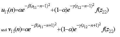
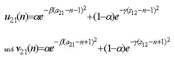
 (1)
(1)
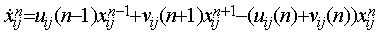
with the boundary conditions uij(N)xNy=vij(-N)xijN=0.
 (2)
(2)
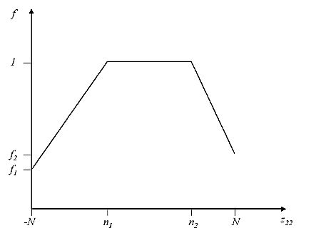
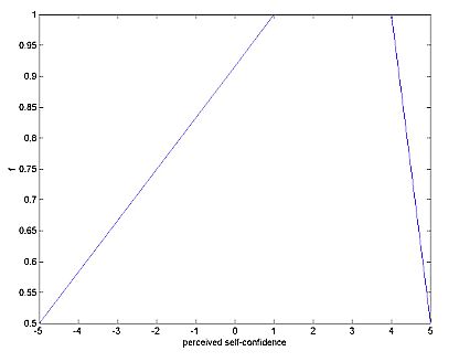
where α11∈[-N,N], α∈[0,1], β≥0 and γ≥0 are parameters and f is a function having a trapezoidal form as shown in figure 2.
|
| Figure 2: Function f |
 (3)
(3)
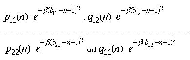 (4)
(4)
Simulation Studies
|
| Figure 3: The particular choice of function f |
|
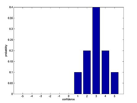
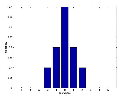
| Figure 4: Initial distribution : biased towards confidence |
|
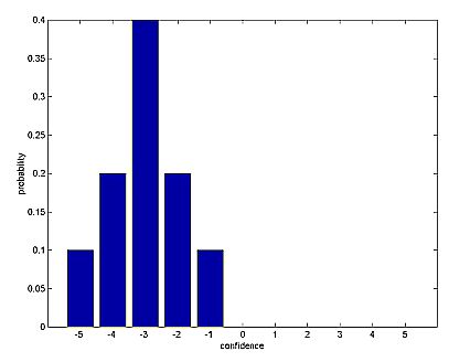
| Figure 5: Initial distribution : biased towards non-confidence |
|
| Figure 6: Initial distribution : neutral confidence |
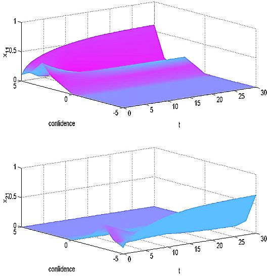
|
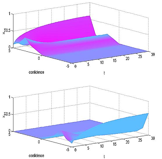
| Figure 7: Simulation results - confidence levels as experienced by individual 1 |
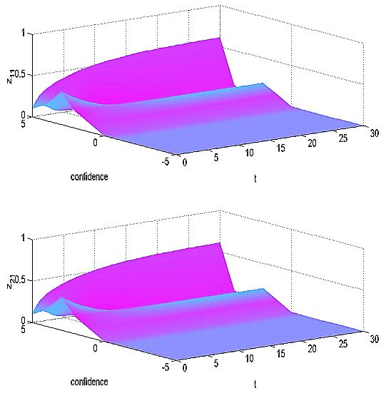
|
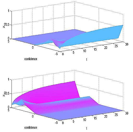
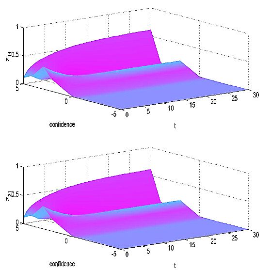
| Figure 8: Simulation results - confidence levels as perceived by individual 1 |
|
| Figure 9: Simulation results - confidence levels as perceived by individual 2 |
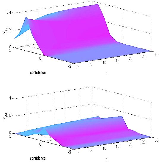
|
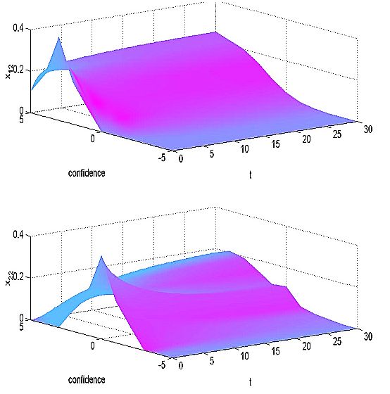
| Figure 10: Simulation results - confidence levels as experienced by individual 2 |
|
| Figure 11: Simulation results - confidence levels as experienced by individual 1 |
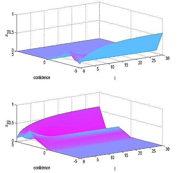
|
| Figure 12: Simulation results - confidence levels as perceived by individual 1 |
|
| Figure 13: Simulation results - confidence levels as perceived by individual 2 |
|
| Figure 14: Simulation results - confidence levels as experienced by individual 2 |
Perspectives
LE CARDINAL, G., GUYONNET, J.-F. and POUZOULLIC (1997), La Dynamique de la Confiance, Dunod.
PEARSON, D.W., ALBERT, P., BESOMBES, B., BOUDEREL, M.-R., MARCON, E. and MNEMOI, G. (2001a), Modelling Enterprise Networks: A Master Equation Approach, to appear European Journal of Operational Research.
PEARSON, D.W. and DRAY, G. (2001b), A Fuzzy Approach to Sociodynamical Interactions, Proceedings International Conference on Artificial Neural Networks and Genetic Algorithms, Prague, Czech Republic.
WEIDLICH, W. and HAAG, G. (1983), Concepts and Models of a Quantitative Sociology, Springer-Verlag.
Annex - Matlab Codes
clear
clf
N=5;
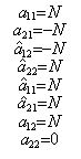
a=[N -N -N N N N N 0];
alpha=[0.9 0.9 1 1 1 1 0.2 0.2];
beta=[2 2 2 2 2 2 2 2];
gamma=[2 2 2 2 0.1 0.1 0.1 0.1];
fp=[1 4 0.5 0.5
1 4 0.5 0.5];
dist1=[0 ; 0 ; 0 ; 0 ; 0 ; 0 ; 0.1 ; 0.2 ; 0.4 ; 0.2 ; 0.1];
dist2=[0.1 ; 0.2 ; 0.4 ; 0.2 ; 0.1 ; 0 ; 0 ; 0 ; 0 ; 0 ; 0];
dist3=[0 ; 0 ; 0 ; 0.1 ; 0.2 ; 0.4 ; 0.2 ; 0.1 ; 0 ; 0 ; 0];
x0=[dist1 ; dist2 ; dist2 ; dist1 ; dist1 ; dist1 ; dist1 ; dist3];
[t,x]=ode45('group_interaction',[0,30],x0,[],a,N,alpha,beta,gamma,fp);
clf
u=-N:N;
for j=1:length(t)
for i=1:2*N+1
z11(i,j)=x(j,i);
z21(i,j)=x(j,2*N+1+i);
zhat12(i,j)=x(j,2*(2*N+1)+i);
zhat22(i,j)=x(j,3*(2*N+1)+i);
zhat11(i,j)=x(j,4*(2*N+1)+i);
zhat21(i,j)=x(j,5*(2*N+1)+i);
z12(i,j)=x(j,6*(2*N+1)+i);
z22(i,j)=x(j,7*(2*N+1)+i);
end
end
for i=1:2*N+1
f(i)=funcf(u(i),fp(1,1),fp(1,2),fp(1,3),fp(1,4),N);
end
% the world as seen by individual 1
figure(1)
subplot(2,1,1)
surfl(t,u,z11)
xlabel('t')
ylabel('confidence')
zlabel('x_{11}')
shading interp
colormap('cool')
subplot(2,1,2)
surfl(t,u,z21)
xlabel('t')
ylabel('confidence')
zlabel('x_{21}')
shading interp
colormap('cool')
figure(2)
subplot(2,1,1)
surfl(t,u,zhat12)
xlabel('t')
ylabel('confidence')
zlabel('z_{12}')
shading interp
colormap('cool')
subplot(2,1,2)
surfl(t,u,zhat22)
xlabel('t')
ylabel('confidence')
zlabel('z_{22}')
shading interp
colormap('cool')
% the world as seen by individual 2
figure(3)
subplot(2,1,1)
surfl(t,u,zhat11)
xlabel('t')
ylabel('confidence')
zlabel('z_{11}')
shading interp
colormap('cool')
subplot(2,1,2)
surfl(t,u,zhat21)
xlabel('t')
ylabel('confidence')
zlabel('z_{21}')
shading interp
colormap('cool')
figure(4)
subplot(2,1,1)
surfl(t,u,z12)
xlabel('t')
ylabel('confidence')
zlabel('x_{12}')
shading interp
colormap('cool')
subplot(2,1,2)
surfl(t,u,z22)
xlabel('t')
ylabel('confidence')
zlabel('x_{22}')
shading interp
colormap('cool')
The various functions called by the main program
function f=funcf(x,n1,n2,f1,f2,N)
if x=n1 &
x
f(1)=f(1)-uij(x,-N,1,3,4,a,N,alpha,beta,gamma,fp(1,1),fp(1,2),fp(1,3),fp(1,4))*x(1);
for n=-N+1:N-1
i=n+N+1;
f(i)=vij(x,n+1,1,3,4,a,N,alpha,beta,gamma,fp(1,1),fp(1,2),fp(1,3),fp(1,4))*x(i+1 );
f(i)=f(i)-vij(x,n,1,3,4,a,N,alpha,beta,gamma,fp(1,1),fp(1,2),fp(1,3),fp(1,4))*x(i);
f(i)=f(i)+uij(x,n-1,1,3,4,a,N,alpha,beta,gamma,fp(1,1),fp(1,2),fp(1,3),fp(1,4))*x(i-1);
f(i)=f(i)-uij(x,n,1,3,4,a,N,alpha,beta,gamma,fp(1,1),fp(1,2),fp(1,3),fp(1,4))*x(i);
end
f(2*N+1)=-vij(x,N,1,3,4,a,N,alpha,beta,gamma,fp(1,1),fp(1,2),fp(1,3),fp(1,4))*x(2*N+1);
f(2*N+1)=f(2*N+1)+uij(x,N-1,1,3,4,a,N,alpha,beta,gamma,fp(1,1),fp(1,2),fp(1,3),fp(1,4))*x(2*N);
% x21
f(2*N+2)=vij(x,-N+1,2,3,0,a,N,alpha,beta,gamma,fp(1,1),fp(1,2),fp(1,3),fp(1,4))*x(2*N+3);
f(2*N+2)=f(2*N+2)-uij(x,-N,2,3,0,a,N,alpha,beta,gamma,fp(1,1),fp(1,2),fp(1,3),fp(1,4))*x(2*N+2);
for n=-N+1:N-1
i=n+3*N+2;
f(i)=vij(x,n+1,2,3,0,a,N,alpha,beta,gamma,fp(1,1),fp(1,2),fp(1,3),fp(1,4))*x(i+1);
f(i)=f(i)-vij(x,n,2,3,0,a,N,alpha,beta,gamma,fp(1,1),fp(1,2),fp(1,3),fp(1,4))*x(i);
f(i)=f(i)+uij(x,n-1,2,3,0,a,N,alpha,beta,gamma,fp(1,1),fp(1,2),fp(1,3),fp(1,4))*x(i-1);
f(i)=f(i)-uij(x,n,2,3,0,a,N,alpha,beta,gamma,fp(1,1),fp(1,2),fp(1,3),fp(1,4))*x(i);
end
f(2*(2*N+1))=-vij(x,N,2,3,0,a,N,alpha,beta,gamma,fp(1,1),fp(1,2),fp(1,3),fp(1,4))*x(2*(2*N+1));
f(2*(2*N+1))=f(2*(2*N+1))+uij(x,N-1,2,3,0,a,N,alpha,beta,gamma,fp(1,1),fp(1,2),fp(1,3),fp(1,4))*x(2*(2*N+1)-1);
% z12
f(2*(2*N+1)+1)=vij(x,-N+1,3,3,0,a,N,alpha,beta,gamma,fp(1,1),fp(1,2),fp(1,3),fp(1,4))*x(2*(2*N+1)+2);
f(2*(2*N+1)+1)=f(2*(2*N+1)+1)-uij(x,-N,3,3,0,a,N,alpha,beta,gamma,fp(1,1),fp(1,2),fp(1,3),fp(1,4))*x(2*(2*N+1)+1);
for n=-N+1:N-1
i=n+2*(2*N+1)+N+1;
f(i)=vij(x,n+1,3,3,0,a,N,alpha,beta,gamma,fp(1,1),fp(1,2),fp(1,3),fp(1,4))*x(i+1);
f(i)=f(i)-vij(x,n,3,3,0,a,N,alpha,beta,gamma,fp(1,1),fp(1,2),fp(1,3),fp(1,4))*x(i);
f(i)=f(i)+uij(x,n-1,3,3,0,a,N,alpha,beta,gamma,fp(1,1),fp(1,2),fp(1,3),fp(1,4))*x(i-1);
f(i)=f(i)-uij(x,n,3,3,0,a,N,alpha,beta,gamma,fp(1,1),fp(1,2),fp(1,3),fp(1,4))*x(i);
end
f(3*(2*N+1))=-vij(x,N,3,3,0,a,N,alpha,beta,gamma,fp(1,1),fp(1,2),fp(1,3),fp(1,4))*x(3*(2*N+1));
f(3*(2*N+1))=f(3*(2*N+1))+uij(x,N-1,3,3,0,a,N,alpha,beta,gamma,fp(1,1),fp(1,2),fp(1,3),fp(1,4))*x(3*(2*N+1)-1);
% z22
f(3*(2*N+1)+1)=vij(x,-N+1,4,3,0,a,N,alpha,beta,gamma,fp(1,1),fp(1,2),fp(1,3),fp(1,4))*x(3*(2*N+1)+2);
f(3*(2*N+1)+1)=f(3*(2*N+1)+1)-uij(x,-N,4,3,0,a,N,alpha,beta,gamma,fp(1,1),fp(1,2),fp(1,3),fp(1,4))*x(3*(2*N+1)+1);
for n=-N+1:N-1
i=n+3*(2*N+1)+N+1;
f(i)=vij(x,n+1,4,3,0,a,N,alpha,beta,gamma,fp(1,1),fp(1,2),fp(1,3),fp(1,4))*x(i+1);
f(i)=f(i)-vij(x,n,4,3,0,a,N,alpha,beta,gamma,fp(1,1),fp(1,2),fp(1,3),fp(1,4))*x(i);
f(i)=f(i)+uij(x,n-1,4,3,0,a,N,alpha,beta,gamma,fp(1,1),fp(1,2),fp(1,3),fp(1,4))*x(i-1);
f(i)=f(i)-uij(x,n,4,3,0,a,N,alpha,beta,gamma,fp(1,1),fp(1,2),fp(1,3),fp(1,4))*x(i);
end
f(4*(2*N+1))=-vij(x,N,4,3,0,a,N,alpha,beta,gamma,fp(1,1),fp(1,2),fp(1,3),fp(1,4))*x(4*(2*N+1));
f(4*(2*N+1))=f(4*(2*N+1))+uij(x,N-1,4,3,0,a,N,alpha,beta,gamma,fp(1,1),fp(1,2),fp(1,3),fp(1,4))*x(4*(2*N+1)-1);
% z11
f(4*(2*N+1)+1)=vij(x,-N+1,5,3,0,a,N,alpha,beta,gamma,fp(2,1),fp(2,2),fp(2,3),fp(2,4))*x(4*(2*N+1)+2);
f(4*(2*N+1)+1)=f(4*(2*N+1)+1)-uij(x,-N,5,3,0,a,N,alpha,beta,gamma,fp(2,1),fp(2,2),fp(2,3),fp(2,4))*x(4*(2*N+1)+1);
for n=-N+1:N-1
i=n+4*(2*N+1)+N+1;
f(i)=vij(x,n+1,5,3,0,a,N,alpha,beta,gamma,fp(2,1),fp(2,2),fp(2,3),fp(2,4))*x(i+1);
f(i)=f(i)-vij(x,n,5,3,0,a,N,alpha,beta,gamma,fp(2,1),fp(2,2),fp(2,3),fp(2,4))*x(i);
f(i)=f(i)+uij(x,n-1,5,3,0,a,N,alpha,beta,gamma,fp(2,1),fp(2,2),fp(2,3),fp(2,4))*x(i-1);
f(i)=f(i)-uij(x,n,5,3,0,a,N,alpha,beta,gamma,fp(2,1),fp(2,2),fp(2,3),fp(2,4))*x(i);
end
f(5*(2*N+1))=-vij(x,N,5,3,0,a,N,alpha,beta,gamma,fp(2,1),fp(2,2),fp(2,3),fp(2,4))*x(5*(2*N+1));
f(5*(2*N+1))=f(5*(2*N+1))+uij(x,N-1,5,3,0,a,N,alpha,beta,gamma,fp(2,1),fp(2,2),fp(2,3),fp(2,4))*x(5*(2*N+1)-1);
% z21
f(5*(2*N+1)+1)=vij(x,-N+1,6,3,0,a,N,alpha,beta,gamma,fp(2,1),fp(2,2),fp(2,3),fp(2,4))*x(5*(2*N+1)+2);
f(5*(2*N+1)+1)=f(5*(2*N+1)+1)-uij(x,-N,6,3,0,a,N,alpha,beta,gamma,fp(2,1),fp(2,2),fp(2,3),fp(2,4))*x(5*(2*N+1)+1);
for n=-N+1:N-1
i=n+5*(2*N+1)+N+1;
f(i)=vij(x,n+1,6,3,0,a,N,alpha,beta,gamma,fp(2,1),fp(2,2),fp(2,3),fp(2,4))*x(i+1);
f(i)=f(i)-vij(x,n,6,3,0,a,N,alpha,beta,gamma,fp(2,1),fp(2,2),fp(2,3),fp(2,4))*x(i);
f(i)=f(i)+uij(x,n-1,6,3,0,a,N,alpha,beta,gamma,fp(2,1),fp(2,2),fp(2,3),fp(2,4))*x(i-1);
f(i)=f(i)-uij(x,n,6,3,0,a,N,alpha,beta,gamma,fp(2,1),fp(2,2),fp(2,3),fp(2,4))*x(i);
end
f(6*(2*N+1))=-vij(x,N,6,3,0,a,N,alpha,beta,gamma,fp(2,1),fp(2,2),fp(2,3),fp(2,4))*x(6*(2*N+1));
f(6*(2*N+1))=f(6*(2*N+1))+uij(x,N-1,6,3,0,a,N,alpha,beta,gamma,fp(2,1),fp(2,2),fp(2,3),fp(2,4))*x(6*(2*N+1)-1);
% x12
f(6*(2*N+1)+1)=vij(x,-N+1,7,6,0,a,N,alpha,beta,gamma,fp(2,1),fp(2,2),fp(2,3),fp(2,4))*x(6*(2*N+1)+2);
f(6*(2*N+1)+1)=f(6*(2*N+1)+1)-uij(x,-N,7,6,0,a,N,alpha,beta,gamma,fp(2,1),fp(2,2),fp(2,3),fp(2,4))*x(6*(2*N+1)+1);
for n=-N+1:N-1
i=n+6*(2*N+1)+N+1;
f(i)=vij(x,n+1,7,6,0,a,N,alpha,beta,gamma,fp(2,1),fp(2,2),fp(2,3),fp(2,4))*x(i+1);
f(i)=f(i)-vij(x,n,7,6,0,a,N,alpha,beta,gamma,fp(2,1),fp(2,2),fp(2,3),fp(2,4))*x(i);
f(i)=f(i)+uij(x,n-1,7,6,0,a,N,alpha,beta,gamma,fp(2,1),fp(2,2),fp(2,3),fp(2,4))*x(i-1);
f(i)=f(i)-uij(x,n,7,6,0,a,N,alpha,beta,gamma,fp(2,1),fp(2,2),fp(2,3),fp(2,4))*x(i);
end
f(7*(2*N+1))=-vij(x,N,7,6,0,a,N,alpha,beta,gamma,fp(2,1),fp(2,2),fp(2,3),fp(2,4))*x(7*(2*N+1));
f(7*(2*N+1))=f(7*(2*N+1))+uij(x,N-1,7,6,0,a,N,alpha,beta,gamma,fp(2,1),fp(2,2),fp(2,3),fp(2,4))*x(7*(2*N+1)-1);
% x22
f(7*(2*N+1)+1)=vij(x,-N+1,8,6,5,a,N,alpha,beta,gamma,fp(2,1),fp(2,2),fp(2,3),fp(2,4))*x(7*(2*N+1)+2);
f(7*(2*N+1)+1)=f(7*(2*N+1)+1)-uij(x,-N,8,6,5,a,N,alpha,beta,gamma,fp(2,1),fp(2,2),fp(2,3),fp(2,4))*x(7*(2*N+1)+1);
for n=-N+1:N-1
i=n+7*(2*N+1)+N+1;
f(i)=vij(x,n+1,8,6,5,a,N,alpha,beta,gamma,fp(2,1),fp(2,2),fp(2,3),fp(2,4))*x(i+1);
f(i)=f(i)-vij(x,n,8,6,5,a,N,alpha,beta,gamma,fp(2,1),fp(2,2),fp(2,3),fp(2,4))*x(i);
f(i)=f(i)+uij(x,n-1,8,6,5,a,N,alpha,beta,gamma,fp(2,1),fp(2,2),fp(2,3),fp(2,4))*x(i-1);
f(i)=f(i)-uij(x,n,8,6,5,a,N,alpha,beta,gamma,fp(2,1),fp(2,2),fp(2,3),fp(2,4))*x(i);
end
f(8*(2*N+1))=-vij(x,N,8,6,5,a,N,alpha,beta,gamma,fp(2,1),fp(2,2),fp(2,3),fp(2,4))*x(8*(2*N+1));
f(8*(2*N+1))=f(8*(2*N+1))+uij(x,N-1,8,6,5,a,N,alpha,beta,gamma,fp(2,1),fp(2,2),fp(2,3),fp(2,4))*x(8*(2*N+1)-1);
f=f';
function f=uij(x,n,k,l,m,a,N,alpha,beta,gamma,n1,n2,f1,f2)
f=alpha(k)*exp(-beta(k)*((n+1-a(k))^2));
if m==0
f=f+(1-alpha(k))*exp(-gamma(k)*((n+1-Exij(x,l,N))^2));
else
f=f+(1-alpha(k))*exp(-gamma(k)*((n+1-Exij(x,l,N))^2))*funcf(Exij(x,m,N),n1,n2,f1,f2,N);
end
function f=vij(x,n,k,l,m,a,N,alpha,beta,gamma,n1,n2,f1,f2)
f=alpha(k)*exp(-beta(k)*((n-1-a(k))^2));
if m==0
f=f+(1-alpha(k))*exp(-gamma(k)*((n-1-Exij(x,l,N))^2));
else
f=f+(1-alpha(k))*exp(-gamma(k)*((n-1-Exij(x,l,N))^2))*funcf(Exij(x,m,N),n1,n2,f1,f2,N);
end
 Return to Contents of this issue
© Copyright Journal of Artificial Societies and Social Simulation, [2001]