© Copyright JASSS


Henriëtte S. Otter, Anne van der Veen and Huib J. de Vriend (2001)
ABLOoM: Location behaviour, spatial patterns, and agent-based modelling
Journal of Artificial Societies and Social Simulation
vol. 4, no. 4
<https://www.jasss.org/4/4/2.html>
To cite articles published in the Journal of Artificial Societies and Social Simulation, please reference the above information and include paragraph numbers if necessary
Received: 17-Apr-01
Accepted: 15-Aug-01
Published: 31-Oct-01
 Abstract
-
This paper presents an Agent-based LOcation Model (ABLOoM). ABLOoM simulates the location decisions of two main types of agents, namely households and firms. The model contains multiple interactions that are crucial in understanding land use changes, such as interactions of agents with other agents, of agents with their environment and of agents with emerged patterns. In order to understand the mechanisms that are at the basis of land use changes and the formation of land use patterns, ABLOoM allows us to study human behaviour at the microlevel in a spatial context. The models, which include economic theory, aspects of complexity theory and decision rules, show that it is possible to generate macrolevel land use patterns from microlevel spatial decision rules.
- Keywords:
-
agent-based modelling, location behaviour, spatial pattern formation
 Introduction
- 1.1
- Why do economic activities cluster? Why do some activities agglomerate into urban environments and why do others show sprawl characteristics? In this article we will deal with these questions through agent-based modelling with complexity as underlying explanatory principle.
- 1.2
- We will first discuss current theoretical principles that underpin the formation of land use patterns. Secondly, we will present a social simulation model for location choice of firms and households based on agent-based modelling.
 Location theory, spatial patterns and ABM
-
Introduction
- 2.1
- At the basis of the formation of agglomerations is the location behaviour of individuals and firms. Regional economics and geography provide theories to deal with these location patterns and location behaviour. Many of these theories are not sufficient to explain the complex spatial patterns, such as clusters and sprawl, that we encounter. Agent-based modelling is a type of simulation modelling that allows us to deal with the formation of these patterns. In the next sections these issues will briefly be summarised.
Regional economics
- 2.2
- Explaining behaviour in a spatial context is part of regional economic literature. We confine ourselves to location theory and the emergence of spatial patterns and structures.
- 2.3
- In location theory a distinction is made between location theories of the firm, location theories of households and the interaction between the two. In the literature on location of the firm, transportation costs (as an estimate of the notion of space and distance) are central to location choice. A distinction is made between models that assume a demand for goods and services continuously dispersed in space and models where demand is concentrated in one point, see (Lloyd and Dicken 1977). The first type of models suggests (Christaller and Lösch type) geographical patterns of firm location that are hierarchical ordered, whereas the second type presents structures that are dependent on the (point) location of markets and resources. (Anas et al. 1998) note that defining clusters in space is not straightforward. The distinction between an organised system of subcentres and apparently unorganised urban sprawl depends very much on the spatial scale of observation.
- 2.4
- In using an urban location model (Alonso 1960) developed a model (based on the ideas of von Thünen in the 19th century) that can be regarded as the foundation for household location choice. Alonso's approach is based on the principle that rents decrease outward from the city centre. Rent gradients consist of a series of bid-rents, which compensate for falling revenue and higher operating costs. Different land uses have different rent gradients, the use with the highest gradient prevailing. Competitive bidding (based on perfect information) determines patterns of rent and allocates specific sites between users to ensure that the highest and best use is obtained. Land is used in the most appropriate way and profit is maximised.
- 2.5
- Criticisms of Alonso's model are first of all that in reality information is incomplete, thus that there is an imperfect market. It also fails to take into account the distinctive nature of buildings and their use, which are not easily changed (lock-in). Other points are the heterogeneity of property, public sector land and spillover-effects of other uses.
- 2.6
- The Alonso model and the literature based on it are characterised by some simplistic assumptions. Employment is centralised in the CBD, there is a dense radial road system and all households have the same taste (Richardson, Button et al. 1997). Moreover, the model is static. Some of these assumptions have been removed (for example Pines 1976, White 1976, Fujita 1976, Fujita 1989, Papageorgiou and Pines 1999), but the theories remain rather general and abstract. To counteract some of the restrictive assumptions of the standard urban model, much work was done on two aspects of land use modelling, namely:
- spatial interaction analysis
- dynamic discrete choice theory.
- 2.7
- Spatial interaction models emerged during the 1960s and 1970s and focused on the flows of information, people and goods in a spatial environment. They are mainly statistical models with the aim of large-scale prediction. The spatial interaction models were mostly based on gravity concepts (Lowry 1964). The work on gravity models has led to the development of entropy maximising models, which provide statistical interpretations of the gravity models (Anas 1987). Examples are the models of Wilson (1970). Both the Lowry and Wilson models can be considered non-economic (Anas 1987). Their rationale is statistical rather than microeconomic. Although the models are macro-oriented and not based on microeconomic principles, they have contributed to the advancement of urban and land use economics.
- 2.8
- While the micro oriented location theory models can be characterised by good behavioural assumptions and poor predictions about spatial interactions, the spatial interaction models have converse characteristics (Macmillan 1993). This lack of behavioural contents led to the study of individual choice behaviour and discrete choice models (Fischer 1991). For a comprehensive overview of the various models, see Clark and van Lierop 1986, Anas 1987, Thisse, Button et al. 1996). While work has been done on dynamic logit models (Nijkamp and Reggiani 1992), many of these models are static models, for example the multinomial logit model. For two reasons, these models have limited usefulness in studying microlevel behaviour in a spatial setting. The first reason is the exclusion of the time aspect (lag between causes and effects) and the second is the lack of interactions between individuals (Haag 1989). These interactions form an important aspect of the ABLOoM approach presented in Section 3.
Complex structures and patterns
- 2.9
- The location theories of Von Thünen and Alonso are not sufficient to explain the real world complex spatial structures that we encounter (Otter 2000). One of the main questions in the literature on the interaction between firms and households is why economic activities seem to concentrate in a (small) number of locations. (Anas et al. 1998) answer this question by referring to alternative assumptions for the Pareto equilibrium of monocentric cities that makes a uniform distribution unstable. Spatial inhomogeneities, internal scale economies, external scale economies and imperfect competition create polycentric agglomerations. In regional economic theory external economies of scale, agglomeration economies, or localisation economies are used as theoretical constructs explaining why firms locate in each other's vicinity to arrive at increasing returns to scale (See Marshall 1890 and Lambooy 1998). Business firms locate in each other's vicinity in order to gain from the attractiveness of companies of the same type activity, but also to gain from the general atmosphere in such a region.
- 2.10
- Krugman (1993) regards these notions as a major contribution to economic theory. However, the theoretical constructs have remained a black box failing to explain the occurrence of spatial structures and patterns on a high level of spatial resolution. In their survey of economic literature on urban spatial structures, (Anas et al. 1998) conclude to their own surprise that non-economic explanations have much more to offer in interpreting the blackbox. Self-organising criticality and synergetics produce organised structures with which the formation of polycentric cities may be explained in a totally different theoretical context than standard neo-classical economics. In these concepts interactions between individual actors as the ultimate expression of complexity may give rise to meso and macro spatial structures.
- 2.11
- Self-organising systems are complex systems which, from a random situation, evolve into an unexpected order. The most important aspect is that, as the term self-organising implies, the system organises itself from within and structures are not imposed from the outside (Prigogine and Stengers 1985). For a system to be self-organising it requires an interaction with its environment and non-linear relations between its elements. The concept of synergetics developed in the 1970's can be considered a sub-field of the self-organisation approach. Haken (Haken 1977; Haken 1996) introduces the term synergetics to indicate the structural self-organising space-time features of multi-component systems.
- 2.12
- The ideas of evolution, self-organisation and synergetics all aim to increase the understanding of complex systems. What use can they have in the application to spatial systems? First of all we mention the concept of cellular automata. With Geographical Information Systems (GIS) geographers have an essential tool at hand to solve questions of spatial patterns (Martin 1996). In recent work progress has been made by applying cellular automata, to convert GIS into a dynamic tool (Tobler 1979, Couclelis 1985; Couclelis 1997). Cellular automata use a set of transition rules that govern the local behaviour at each cell with respect to the cell's neighbours. It offers a means to study emergent global behaviour in systems where only local processes are understood (Engelen, et al. 1995, White and Engelen 1994, Hegselmann and Flache 1998). Recently, there are good examples of the use of GIS in combination with ecological dynamics and agent behaviour in Bousquet, et al. ( 2001) and Weisbuch ( 2000).
- 2.13
- Secondly, there is an increasing number of examples of models of 'complexity' that have been applied to the problems of socio-economic dynamics. We refer to Pumain ( 1989), Arthur, Durlauf et al. ( 1997) and Nijkamp and Reggiani ( 1998) for overviews of models of complexity in economics. While the concepts of 'complexity' themselves are not new, the application of these concepts to socio-economic processes is a relatively new phenomenon. There are a number of examples in the field of regional sciences in applying these theoretical concepts including residential location (Dendrinos and Haag 1984), migration (Haag and Weidlich 1984) and models to explain the sudden growth of cities or 'shocks in urban evolution' (Haag 1989). Moreover, Krugman ( 1996) applies self-organising principles to spatial economies. He presents an approach to clarify the emergence of edge cities (office districts) in polycentric metropolitan areas. Finally, Allen ( 1997) presents self-organising models of urban and regional systems. The work of Allen et al. stems from the early work of Prigogine and has become known as the Brussels School. The self-organising models aim to show how structures evolve as a result of human decision making, involving cultural, social, economic and environmental factors. The models describe the growth of cities and regions along paths of non-equilibrium. In ABLOoM (Section3) a different approach will be taken as spatial behaviour of individual agents will be modelled.
Clusters and sprawl
- 2.14
- In this study we focus on two distinct land use patterns, namely clusters and sprawl. Patterns of clustering and sprawl are known in the literature by a variety of terms.
- 2.15
- Clusters emerge in the context of external economies of scale, which we call 'agglomeration economies'. The rationale behind agglomeration economies is that companies are attracted to each other and benefit from being close to input sources or to their markets depending on the type of industry. The term 'clusters' is used to indicate two different agglomeration phenomena, namely localisation economies and urbanisation economies. Localisation economies indicate geographic concentrations of interconnected companies and institutions in a particular field (Hoover 1971; Lambooy 1981; Lambooy, Wever and Atzema 1997). The second meaning of the term 'cluster' refers to urbanisation economies, which are also known as urban agglomerations (Hoover 1971; Krugman 1996; Lambooy, Wever and Atzema 1997; Lambooy 1998). Urbanisation economies emerge when dissimilar companies, but also households, locate near to each other.
- 2.16
- The term 'sprawl' is the result of a process of 'dispersion'. Dispersion occurs when households and firms wish to stay away from each other. There has been less research on sprawl patterns than on clustering patterns. For studies on 'sprawl' patterns in the US we refer to (Irwin and Bockstael 1998).
 ABLOoM: Agent-based LOcation Model
-
Introduction
- 3.1
- Agent-based modelling is a type of simulation modelling (Epstein and Axtell 1996). In this approach social structures and group behaviour emerge from the interaction of individuals operating in artificial environments. Agents are capable of making decisions based on a set of rules, but they can also exhibit some degree of 'learning' or adaptation. The agent idea allows us to develop a range of different agents with varying behavioural complexity. Recent publications are (Arthur 1994, Axelrod 1997, Gilbert 1996, Gilbert and Troitzsch 1999, Conte, Hegselmann and Terna 1997, Tesfatsion 1998, Liebrand, Nowak and Hegelsmann 1998).
- 3.2
- We have developed an agent-based model that helps us to explore the issue of microlevel land use decisions that drive macrolevel pattern formation (Otter 2000). The theoretical basis of the models is formed by combining three elements. The models are based on:
- spatial human behaviour;
- regional economic concepts;
- decision rules.
- 3.3
- The agents are the driving force in agent-based models, they are the micro elements which drive the macro patterns. The general characteristics of these agents are that they:
- are heterogeneous
- make decisions based on rules
- interact with their environment
- interact with other agents
- can learn from earlier experience
|
|
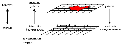
Figure 1. Conceptualisation of an agent-based model
|
- 3.4
- Figure 1 shows a conceptualisation of an agent-based land use model, in which households and firms agent search for a location. It includes a microlevel at which the interactions take place and a macrolevel at which patterns emerge. These macroscopic patterns in their turn affect the behaviour on a microlevel.
- 3.5
- The Swarm modelling platform (Minar et al., 1996; Langton et al., 1997) was used to build our agent-based models (Otter 2000). The main advantage of Swarm is that it offers an object-oriented standardised set of software tools, that could be readily used and implemented into our own models. This significantly reduces programming efforts. The Swarm version (V 2.0.1) that was used runs on a PC and is based on the Java programming language.
- 3.6
- Before presenting the actual models, the general structure of the models, as well as some important methodological issues, are introduced and discussed in the next sections. The models consist of a grid, a number of agents and the rules which make them act.
Grid
- 3.7
- The grid (or lattice) in our model includes 101×101 cells. On the screen the grid appears to be a square grid with fixed boundaries, but it is actually a torus. The grid is composed of many layers of different types of data, but only one layer is represented. The layers can be 'read' at any time by the agents, they can withdraw values from the cells with which they interact and they can also restore values in the grid.
- 3.8
- One of the layers in the model is the initial 'land use' layer, which consists of three types of environmental attributes, namely 'land', 'natural area' and 'sea'. These attributes are fixed and the initial grid is considered empty implying that no agents have located in it. Agents are only allowed to locate in empty cells that are labelled 'land'. While agents can not locate in 'natural area' or 'sea', they can be attracted to these environmental features depending on their decision rules. The cells that are occupied by agents remain of the type 'land', but merely change from empty to occupied. In cases where agents leave a location to search for a new location, the cell is changed back from occupied to empty.
- 3.9
- A second type of layer is the ' attraction' layer. The concept of attraction is introduced to simulate agglomeration phenomena. The rationale behind agglomerations is that some agents, whether households or firms, benefit from being close to each other. Firms are attracted to each other for a number of reasons. Similar firms or shops can be attracted by the presence of markets and potential customers, while dissimilar firms can benefit from delivering goods and services to each other. Households can be attracted to each other for a number of reasons, such as social contacts, the quality of the neighbourhood or the presence of schools and shops. These agglomeration effects are translated into an attraction variable. The attraction variable is one of the multiple issues that agents take into account when making location decisions based on a set of rules (see section 3.5).
- 3.10
- 'Attraction' is presented here as a characteristic of the environment, as opposed to an agent characteristic, since it is the location that attracts agents. The 'attraction' symbolises the positive interaction force that is created by the presence of agents, which pulls other agents towards the area. The 'attraction' of a location is not fixed; the agents continuously affect it during the simulation. In our model, a different attraction 'layer' is introduced for each type of agent. Depending on the type of agent involved, it has a varying degree of sensitivity to attraction of other types of agents. Firms can also attract households and vice versa. One of the major reasons for this attraction is given by employment opportunities. Jobs attract people and more people create more jobs (Pumain 1989; Allen 1997). As an example households will be more attracted to light industry, because of employment chances, than to heavy industry. These differences are reflected in the decision rules of the agents. Conversely, agents may repel rather than attract each other.
Methodological issues
- 3.11
- In our models an agent represents a household or a firm, which is searching for a location. An agent can have any of two states. It is either searching for a location and therefore 'unsettled', or it has found a location and is therefore 'settled'.
- 3.12
- A methodological aspect in this context concerns the way the agents are assigned to the grid. The 'unsettled' agents that are 'searching' for a location which suits their requirements, have to start from an initial position. There are a numerous ways of assigning this initial starting position. One possibility is to let all agents start their activity in position (0,0). Another possibility is to include some degree of randomness by letting them start along one of the edges of the grid, for instance (0,y). Both these options have been tried in a variety of simulations. We can conclude that the starting position of the agents affects the outcome of the model. Especially if agents have a limited radius in which they can act[1], the initial position of the agents largely affects the pattern formation in the models. In other words, the results are sensitive to the starting position of the agents. To minimise this effect in our models, the agents obtain a random initial position on the grid. This is achieved through a uniform distribution in which all locations have an equal probability of being chosen. Since the results of the simulation are sensitive to the initial position of the agents, using a random allocation of the agents to the grid, reduces the overall effect of the initial positions.
- 3.13
- An additional point is that a maximum of one agent is allowed to locate in each cell. If an agent moves to a location, it is then considered to be occupied. As more agents settle, this leads to the emergence of patterns on the grid. The other option is to allow for multiple agents to stay in one cell, but then the form of the pattern will not be known and valuable information may be lost. In addition, this way of modelling also disguises the space requirements of location behaviour.
- 3.14
- A second methodological issue concerns the 'starting time' of the agents. The agents are 'activated' at a certain time, and the timing of this event may influence the results of the model. A timestep in the model does not represent a specific time in reality. There are a number of options for handling starting time, and we have investigated the following. A first option is to activate all the agents at once. Thus, in one timestep all agents are given their initial position from which they start searching for their optimal location. This works fine in relatively simple models, but leads to problems in more complex simulations, especially when interactions between agents are included. If an agent's behaviour depends on the behaviour of other agents, a situation may arise in which agents are endlessly waiting for each other to act. Another option is to activate the agents sequentially, but on fixed starting times. A drawback is that the models become very rigid. Yet another option is to provide the agents with a random starting time. In this case, all agents choose their starting time randomly according to a uniform distribution, from a specified range. Here too we may encounter the problem of agents that are endlessly waiting for each other to act. This occurs when an agent, whose behaviour depends on that of another agent, starts before the agent that it reacts upon. All three options that are presented here have drawbacks that occur in specific situations. As a solution, a combination of these ways to handle the starting times of the agents was used.
- 3.15
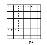
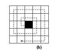
- A third methodological issue is the way the agents search the grid for an optimal location. In our models, some agents are required to search the grid for a specific location, agent or phenomenon, depending on their decision rules. The 'neighbourhood' in which they can act is also specified in the decision rules. There are basically two search mechanisms that agents can employ. In each model we specify which search mechanism will be used by the agents. The first search mechanism scans the entire grid, from the top left corner to the lower right corner. In this case, each cell is in the grid can be 'analysed' by the agent. In a way it is a macrolevel analysis of what is present on the grid. The second search mechanism is micro-oriented. In this case agents search in an area around their current location. They do so by following a 'circular' search pattern. Both search mechanisms are presented in Figure 2.
|
|
Figure 2. Search mechanisms (a) for the entire grid and (b) from an initial position
|
- 3.16
- All of our agents are given a set of rules, which determine their behaviour in every situation. These rules can have a variety of appearances and act on various scales. The different decision rules in our models can be:
- autonomous: The agents start behaving in a certain manner as soon as the agent is activated. This simulates the autonomous behaviour of individuals that is independent of external stimuli.
- time-dependent: The agent's actions are activated only after a specified period of time.
- environment dependent: The agent's behaviour depends on the characteristics of the environment in which it operates.
- based on interaction with other agents: The agent's behaviour is a reaction to the actions of other agents. In the model we include household-household interactions, firm-firm interactions and household-firm interactions.
- based on interaction with the macro patterns: The agent's behaviour is a reaction to the macro structures and patterns that have emerged.
In each of the simulations the agents' decision rules will be elaborated upon.
Agents
Introduction
- 3.17
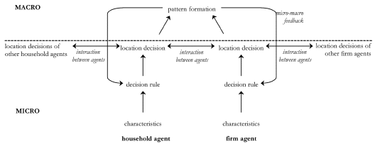
- In ABLOoM, the location decisions of two main types of agents, namely households and firms, are simulated (Otter 2000). The model contains the multiple interactions that were presented before as being crucial in understanding land use changes. These include interactions of agents with other agents, of agents with their environment and of agents with emerged patterns. A conceptualisation of the agent-based land use model is given in Figure 3.
|
|
Figure 3. Conceptualisation of an agent-based model for land use changes
|
Preferences of households
- 3.18
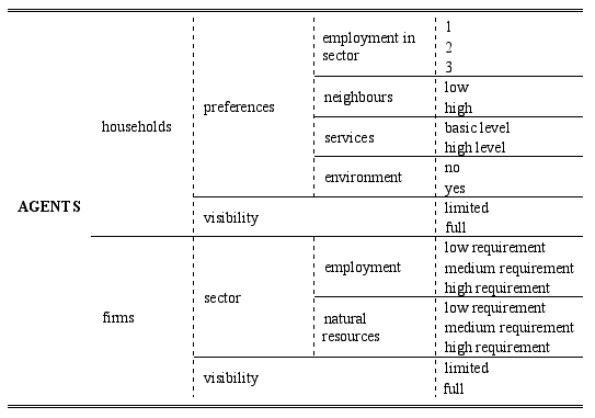
- Each household has its own characteristics by which it can be distinguished. The characteristics of our agents differ from traditional representations of households in a number of ways. In the dominant neoclassical model of studying human behaviour, individuals (and households) are assumed to show optimising rational behaviour based on perfect information. In our agent-based models, agents do not display optimising behaviour, but satisficing behaviour (Simon, 1992). This implies that due to their perception of reality, as well as due to goals, expectations, hopes and beliefs, the agents have preferences for specific locations. The decision rules of each agent are based on these preferences for specific locations. The preferences reflect the characteristics of the households. These characteristics, which can change over time, include household income, age structure, presence of children etc. but also perceptions, myths and meaning. Not all of these characteristics are included explicitly. The characteristics of each household agent are translated into:
- a preference for employment, neighbours, service levels and environment;
- a visibility.
- 3.19
- Concerning employment, it is assumed that (one member of) every household is employed in any of three employment sectors. We distinguish between the heavy industry (sector 3), manufacturing (sector 1) and the service sector (sector 2). It is also assumed that the income range of the households is determined by the sector in which they are employed. As a simplification agents employed in the heavy industry have low incomes, those in manufacturing have medium incomes and those working in the service sector have high incomes. The income of a household is one of the characteristics that is translated into its preference for locations. In addition to the influence through 'income', we assume that the employment of the agents also directly affects their locational wishes. The location of the employment opportunities of agents is important, since it affects the travel time to work (Evers and Van der Veen, 1986, Van der Veen and Evers 1983). This is reflected in the decision rules.
- 3.20
- The preference for neighbours is closely linked to the 'attraction' variable that was introduced earlier. The rationale of a preference for neighbours is based on the fulfilment of basic needs. Being close to others can fulfil 'social' needs such as gaining respect and having a sense of 'belonging' (cf. Maslow, 1954). The wish to be close to other agents is also linked to the 'neighbourhood' effects that we find in the literature (Clark and Van Lierop, 1986). We assume that most households wish to be close to other households since they are social creatures that need contact with other people. Yet, for diverse reasons, some households will wish to be away from others. Consequently, in our model agents can have either a low or high preference for neighbours.
- 3.21
- For service levels, a distinction is made between preferences for basic and high service levels. The concentration of population will promote a level of services (Harvey, 1996). A small concentration is assumed to lead to basic service levels, for example the presence of school, shops etc. Larger concentrations lead to high service levels, represented by the presence services such as theatres, libraries, hospitals etc. These services are most commonly found in larger cities. In this model service levels are regarded as an emergent property, since they depend on the size of the clusters of agents (see also Christaller, 1933). We assume that for high service levels a minimum population of agents must be present. In these simulations a 'cluster' is defined as an agglomeration of minimally 5 agents.
- 3.22
- The environment preference was included to indicate the 'natural' value of certain zones and to provide the basis for interactions between humans and nature. The preference for environment represents the wish of agents to live in a location with a high environmental quality. It is expressed in the decision rules as the distance to natural areas. In addition, the natural environment can be used as an input source for the production of goods. Certain input-oriented firms are therefore assumed to have a preference to be close to a natural resource.
- 3.23
- Apart from the preferences for employment, neighbours, service levels and the environment, the second characteristic of the agents is that they possess a'visibility'. The concept of 'visibility' is included to simulate the effects of a bounded rationality. Visibility in our model is represented as a radius, which the agents use to search the locations around them, starting from their initial position. Since the agents use a 'circular' search mechanism a full visibility resembles a circle that encompasses the entire grid. Due to the fact that the grid is torus-shaped and consists of 101$times;101 cells, we define a full visibility as a radius of 51 cells. Circles with smaller radii then represent lower visibilities. The 'visibility' variable is included for two reasons. The first is to counteract the economic assumption of perfect information, which cannot be held in reality. Our visibility varies from one agent to the next and thus indicates the visible range that agents have for choosing a new location. It represents how far around households and firms are willing to look for a new location. The 'visibility' is also included for a second reason. It is closely linked to the income of a household. When searching for a location high income households can afford to search in a larger area. Not only can they spend more money on acquiring the information they need, they can afford to live further away from their employment and spend more money on commuting. The introduction of the concept of 'visibility' to our models has far-reaching consequences for the emerging patterns.
Preferences of firms
- 3.24
- In addition to household agents we included firm agents in our model. Each firm has its own characteristics by which it can be distinguished. Similar to the household agents, the characteristics of our firm agents differ from the traditional representations. In the traditional models firms locate where profit are maximal, or where costs are minimised. Yet, other factors, related to the concepts of attraction and repulsion, also play a role in firm location behaviour. In our model each firm agent is equipped with the following characteristics:
- the sector to which it belongs
- a visibility
- 3.25
- The firms originate in three sectors, namely the heavy industry, manufacturing and the service sector. The production of goods in each of these sectors is translated into a requirement for inputs. Two types of input requirements are distinguished, i.e. for employment and for natural resources. Depending on the production characteristics, the requirements for employment and natural resources are specified. Each type of firm can have low, medium or high employment requirements and low, medium or high resource requirements. These requirements greatly affect the location choice of firms. Consider, for example, internet companies that are driven primarily by human capital and have no requirement for natural capital. Note, however, that at this stage we are not able to include a sophisticated process of rule generation by firms as do (Ballot and Taymaz 1999).
- 3.26
- In Table 1 all possible agent characteristics are schematised, for the households and firms. In our model, eight different types of agents are distinguished. These consist of five types of household agents and three types of firm agents. All agents possess a combination of characteristics presented in Table 1.
|
|
Table 1: Agent characteristics
|
- 3.27
- The agent characteristics are translated into decision rules for each type of agent. In the following section the agents and their decision rules are presented.
Rules
- 3.28
- The large number of different agents implies that the rules that we have included are also very diverse. The following agents, their main characteristics and the rules that guide their decision making are distinguished.
Household1
Household1 agents can be considered 'pioneer' agents. They are the first to settle and form the basis for further development.
-
Search for a random location
- If the chosen location is vacant, move there.
Else repeat rule 1
- Update the attraction of the chosen location and the surrounding cells
Household2
- 3.29
- Household2 is assumed to be a low-income household. Agents of this type find employment in either the manufacturing or the heavy industry sector (sector 1 or 3). The sector in which they are employed is randomly assigned to them. Additional assumptions are that the agents wish to live close to other agents, live close to their work, have a preference for basic service levels and no preference for environmental quality.
- Search for the location with the highest attraction value
- Set this value as target attraction
- Search for employment opportunities
- If more locations have identical attraction values, choose the location that is closest to an employment opportunity
- If chosen location is vacant, move there.
Else, move to the nearest vacant location
- Update the attraction of the chosen location and the surrounding cells
- 3.30
- A time-dependent characteristic is also included. After some time Household2 changes its preferences from basic to high service levels (defined as a cluster > 5 agents). To simulate the ageing of agents and resulting changing preferences, a change in preference from basic to high service levels is assumed.
- Search for the nearest location with high service levels (cluster)
- In cluster, search for highest attraction
- Set value as target attraction
- If more locations within this cluster have identical target attraction values, find nearest vacant location
- If chosen location is vacant, move there.
Else, decrease target attraction by 1 and continue with rule 2
- Update the attraction of the chosen location and the surrounding cells
Household3
- 3.31
- Household3 is assumed to be a high-income household. Agents of this type find employment in either the manufacturing or the service sector (sector 1 or 2). The sector in which they are employed is randomly assigned to them. Additional assumptions are that the agents wish to live close to other agents, live close to their work, have a preference for high service levels and a preference for environmental quality. While Household3 has a preference to live in the vicinity of employment opportunities it does not want to live close to too many firms. The agents keep checking the environment for existing firms. If there are too many firms in the neighbourhood Household3 moves to new location according to its initial rules.
- Search for a location with high service levels (cluster)
- If more locations have high service levels, choose the location that is closest to environment and to employment
- In cluster, search for highest attraction
- Set value as target attraction
- If more locations within this cluster have identical target attraction values, find nearest vacant location
- If chosen location is vacant, move there.
Else, decrease target attraction by 1 and continue with rule 4
- Update the attraction of the chosen location and the surrounding cells
- Continue searching for firms
- If number of firms > 10, continue with rule 1
Household4
- 3.32
- Household4 is mainly driven by a high preference for environment. This agent searches for a location that is close to nature.
- Search for a location which is nearest to nature
- If more locations are close to nature, choose one randomly
- If chosen location is vacant, move there.
Else, move to nearest vacant location
- Update the attraction of the chosen location and the surrounding cells
Household5
- 3.33
- Household5 is mainly driven by a repellence of other agents. It wishes to find a location with a certain minimal distance to other agents.
- Search for a location with a minimal distance of 10 cells to any other agent
- If chosen location is vacant, move there
- Continue with rule 1
Firm1
- 3.34
- Firm1 represents a firm in the manufacturing sector. This firm has average employment requirements and average natural resource requirements. It searches for new labour among those employed in sector 1, but also needs natural resources. Two different types of Firm1 are distinguished. The first type of the firms wishes to find a location that is in between clusters of households (cities) and natural resources. The second type of firms locates where the attraction (for this firm) is highest.
- If first group,
- Search for a location with high service levels (cluster)
- If there are more clusters, calculate the distance from each cluster to a natural resource base
- Set cluster which is closest to natural resource base as target cluster
- Choose the location where total distance from target cluster to natural resource base is minimal
- If chosen location is vacant, move there.
Else, move to nearest vacant location
- Update the attraction of the chosen location and the surrounding cells
-
If second group,
- Search for locations with the highest attraction value for this type of firm
- Set this value as target attraction
- If more locations have identical attraction values, choose one randomly
- If chosen location is vacant, move there.
Else, decrease target attraction by 1 and continue with rule 3
- Update the attraction of the chosen location and the surrounding cells
Firm2
- 3.35
- Firm2 represents a firm in the service sector. This firm has high employment requirements and no natural resource requirements. Searches for new labour among those employed in sector 2. Wishes to locate where there is plenty of labour. Again, two different types of Firm2 are distinguished. The first set of firms searches for the highest (household) attraction and high service levels. The second set of firms that locates where attraction is highest.
-
If first group,
- Search for a location with high service levels (cluster)
- If more locations have high service levels, choose the nearest
- In cluster, search for highest attraction
- Set value as target attraction
- If more locations within this cluster have identical target attraction values, find nearest vacant location
- If chosen location is vacant, move there.
Else, decrease target attraction by 1 and continue with rule 5
- Update the attraction of the chosen location and the surrounding cells
-
If second group,
- Search for locations with the highest attraction value for this type of firm
- Set this value as target attraction
- If more locations have identical attraction values, choose one randomly
- If chosen location is vacant, move there.
Else, decrease target attraction by 1 and continue with rule 3
- Update the attraction of the chosen location and the surrounding cells
Firm3
- 3.36
- Firm3 represents a firm in the heavy industry sector. This firm has low employment requirements and high natural resource requirements. Searches for new labour among those employed in sector 3. The first set of firms locates where total distance to natural resource is minimal. Updates attraction for this type of firm surrounding cells. The second set of firms that locates where attraction (for this firm) is highest.
-
If first group,
- Search for a location which is nearest to nature
- If more locations are close to nature, choose one randomly
- If chosen location is vacant, move there.
Else, move to nearest vacant location
- Update the attraction of the chosen location and the surrounding cells
-
If second group,
- Search for locations with the highest attraction value for this type of firm
- Set this value as target attraction
- If more locations have identical attraction values, choose one randomly
- If chosen location is vacant, move there.
Else, decrease target attraction by 1 and continue with rule 3
- Update the attraction of the chosen location and the surrounding cells
- 3.37
- In this first run of the model all agents are assumed to have full information, i.e. full visibility. The initial values and conditions of the model are presented in Table 2.
|
| Table 2: Initial values for ABLOoM |
|
| Type | Number of agents | colour of agents | starting interval |
| Household1 | 10 | red | (3-5) |
| Household2 | 40 | black | (10-60), (starttime+50-120) |
| Household3 | 40 | blue | (40-90) |
| Household4 | 10 | cyan | (6-60) |
| Household5 | 10 | green | (6-60) |
| Firm1 | 25 | orange | (6-20), (30-50) |
| Firm2 | 10 | yellow | (6-20), (30-50) |
| Firm3 | 10 | grey | (6-20), (30-50) |
|
- 3.38
- Table 2 presents three initial values for the agents in the simulation. These are the number of agents that are included of each type, the colour by which the agents can be identified on the grid and their starting time interval. The starting time is the time at which the agents turn 'active', thus at which they are included in the model. 'Time' in the model does not represent a specific time in reality, a timestep represents a calculation round. In ABLOoM, the starting time is picked randomly by each agent from a time interval, which is determined by the modeller. This implies that, rather than all agents of one type having the same starting time, individual agents of the same type are generally activated on different starting times within a specific interval.
- 3.39
- For various types of agents multiple time intervals are presented. For Household2 this represents the time-dependent characteristic. It simulates that these agents grow older and it is assumed to be accompanied by a change in preferences. Therefore, a second time interval is introduced in which the agents change their behaviour (cf. description Household2). For Firm1, Firm2 and Firm3, the second time interval represents the starting time of the second set of agents, which respond to the behaviour of the first set of agents (cf. description Firm1, 2 and 3).
Results of ABLOoM (full visibility)
- 3.40
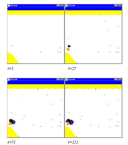
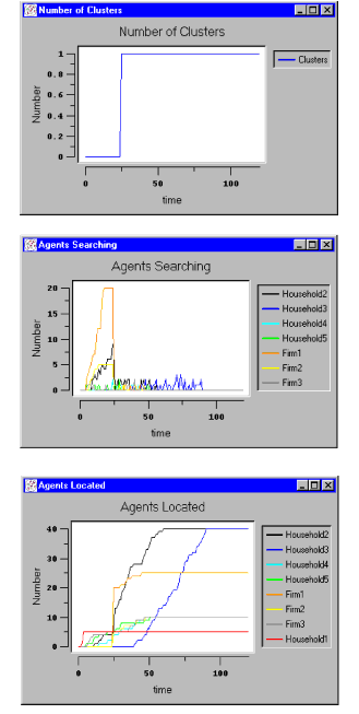
- The results of the simulation model are presented in Figure 4 and Figure 5. Figure 4 shows the emerged land use patterns as they appear on the grid on various moments in time during the simulation. Figure 5 shows the accompanying graphs for the macro level features.
|
|
Figure 4. Results of ABLOoM (full visibility)
|
|
|
Figure 5. Macrolevel features of ABLOoM (full visibility)
|
Analysis of ABLOoM (full visibility)
- 3.41
- The land use decisions of the agents in ABLOoM, generate a colourful land use pattern. In the model we have included rules that are autonomous, time-dependent or based on interaction with other agents and with emerged phenomena. These rules drive the evolution of the system. The rules lead to three land use 'phases' which we clearly observe in our results. The three successive phases are:
- an initial development phase
- a growth phase
- a stable or dynamic equilibrium phase
- 3.42
- The initial development phase is the phase in which a relatively small number of agents has found a location (e.g. Figure 4, t=5). In the growth phase a larger number of agents has found a location and this development influences the location decisions of the agents that are still searching (e.g. Figure 4, t=27 and t=71). In the last phase all agents have settled on the grid. In this specific run of the model all agents have settled around t=88, as can be seen in Figure 5 (Agents Searching/Agents Located). This does not automatically imply that a static equilibrium has been created, in the sense that all agents will stay at their chosen location after this time. Agents can still move around depending on their decision rules. In that case there is still some dynamics in the model and therefore we call it a dynamic equilibrium. In Figure 4, apart from Household1 (red), Household4 (cyan), Household5 (green) and Firm3 (grey), all agents have ended up in one large cluster. We have the following explanation.
- 3.43
- Household1 agents are the first agents to be activated who randomly search for a location. These agents can be found randomly spread over the grid, during the initial development phase. They represent the 'pioneer' agents that enter an empty grid, analogous to the pioneers of early times that discover new land on which to settle. Some of these (mostly agrarian) settlements grew larger and turned into present day cities, while others remained small. This development can also be seen in the simulation results in Figure 4. Only one location initially chosen by a Household1 agent has turned into a city, others remain rather remote.
- 3.44
- There are reasons for Household4 and Household5 agents not being close to a cluster. Household4 agents have a high preference for the environment and so they search for locations that are close to natural areas. In this particular simulation these agents have found locations, which are relatively far away form, the cluster of activities. Chance plays a role here, since Household4 agents do not have a preference to be far away from other agents. If the cluster of activities had been formed close to nature, a situation might have occurred in which Household4 agents had located close to the cluster, or had even become part of the cluster. Household5 agents, on the other hand, are repelled by other agents. These agents can be found spread on the grid, with a certain minimum distance to other agents. They will never be part of a cluster. Household5 agents continuously keep an eye on their environment, and they will move if other agents in the neighbourhood come too close.
- 3.45
- Firm3 agents are firms that act in a very similar manner to Household4 agents. These firms require natural resources as an input for their production and can therefore also be found close to natural areas. Like Household4 agents, Firm3 agents can become part of a cluster by chance.
- 3.46
- Summarising, the four types of agents that have been discussed so far (Household1, Household4, Household5 and Firm3), are not part of the large cluster found in Figure 4. On the contrary, these agents together form a sprawl pattern.
- 3.47
- In the growth phase of the simulation we see that a cluster is being formed by agents of type Household2 (black), Household3 (blue), Firm1 (orange) and Firm2 (yellow). These agents are drawn towards each other for different reasons. Household2 agents are looking for employment opportunities in the manufacturing (Firm1) or heavy industry (Firm3) sector. Firm3 agents are not part of the cluster that is formed in Figure 4, so Household2 is mainly attracted by Firm1 agents. On the other hand, Firm1 and Firm2 agents are looking for labour. Firm2 agents represent firms in the service sector that have high employment requirements. Therefore they search for clusters of activity where they hope to find new labour (in this case under Household2 agents). Firm1 agents, on the other hand, have input requirements in terms of both employment and natural resources. We observe that these firms locate in between the labour source (cluster) and the natural resources (see Figure 4, t=27). In a later phase (see Figure 4, t=71) the Firm1 agents are being absorbed by the cluster.
- 3.48
- In the final phase of the simulation (see Figure 4, t=121), all agents have settled on the grid. Yet, some movement can be observed. The Household3 agents (blue) are still moving around. They wish to move if there are too many (>10) firms in their surroundings. In this simulation, Household3 agents are part of large clusters that include many firms. However, they have difficulty to find a new location since they wish to be close to a cluster due to their preference for high service levels.
Results of ABLOoM (limited visibility)
- 3.49
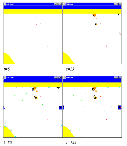
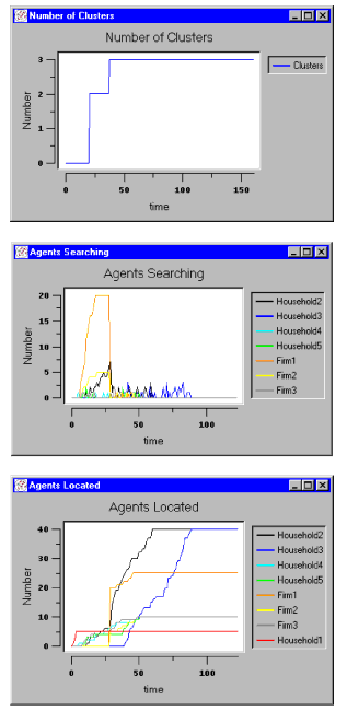
- The results found in the previous section change drastically, if a 'limited visibility' for one particular agent is included. The simulation includes the same number of agents as before and also employs the same starting times for the agents (see Table 2). Household2 is given a visibility of 35 grids in his surrounding. All other agents retain full visibility. In Figure 6 the emerged land use patterns are visualised presented whereas in Figure 7 the macrolevel features are presented.
|
|
Figure 6. Results of ABLOoM (limited visibility)
|
|
|
Figure 7. Macrolevel features of ABLOoM (limited visibility)
|
- 3.50
- Figure 6 and Figure 7 show the effects of reducing the visibility of Household2 agents from full visibility (=51) to 35. Instead of one large cluster, three smaller clusters eventually develop. Due to their lower visibility, Household2 agents search for a location in a smaller area, starting from their initial position. Within that area they choose a location which fits their needs. They settle spread across the grid, this attracts agents of other types and multiple clusters start to grow (see Figure 6, t=23). Similar to the previous example, in which all agents had full visibility, the first clusters to develop in the present simulation consist of agents of the types Household2, Household3, Firm1 and Firm2. This is explained by the fact that these agents have the same decision rules as they had in the previous example. Although all other agents have full visibility, the spreading of Household2 agents leads to the development of multiple clusters. The Household3 agents (blue) all locate in one cluster (see Figure 6, t=122), which is away from the other clusters. They wish to be close to other agents, close to their work and have a preference for high service levels and environmental quality. These wishes could drive them towards the other clusters, but what drives them away is that they do not want to live close to too many firms.
 Conclusion
- 4.1
- In order to understand the mechanisms that are at the basis of land use changes and the formation of land use patterns, we studied human behaviour at the microlevel in a spatial context. In current regional economic literature the microlevel has been underexposed. We have introduced agent-based modelling techniques to help us to link micro and macrolevel of analysis. The agent-based models that we have presented provide an illustration of how to approach land use change issues from the microlevel. The models, which include economic theory, aspects of complexity theory and decision rules, show that it is possible to generate macrolevel land use patterns from microlevel spatial decision rules.
 Notes
Notes
-
1 This concept will be introduced as 'visibility' in a later section.
 Acknowledgement
-
The authors gratefully acknowledge the programming support of René Buijsrogge (University of Twente).
 References
-
ALLEN, P. M. (1997). Cities and Regions as Self-Organising Systems; Models of Complexity. Amsterdam: Gordon and Breach Science.
ALONSO, W. (1960). A Theory of the Urban Land Market. Papers and Proceedings of the Regional Science Association, Vol. 6, 149-157.
ANAS, A. (1987). Modeling in Urban and Regional Economics. Chur [etc.]: Harwood Academic Publishers.
ANAS, A., ARNOTT, R., and SMALL, K. A. (1998). Urban Spatial Structure. Journal of Economic Literature, Vol XXXVI, 1426-1464.
ARTHUR, W. B. (1994). Increasing Returns and Path Dependence in the Economy. Economics, Cognition, and Society Series. Ann Arbor: University of Michigan Press.
ARTHUR, W. B., DURLAUF, S. N., and LANE, D. A. (1997). The Economy as an Evolving Complex System II. Reading: Addison-Wesley.
AXELROD, R. (1997). Advancing the Art of Simulation in the Social Sciences, in: Simulating Social Phenomena. Lecture Notes in Economics and Mathematical Systems, Vol. 456. R. Conte, R. Hegselmann, and P. Terno (eds). Heidelberg and New York: Springer, 21-40.
BALLOT, G., and TAYMAZ, E. (1999). Technological Change, Learning and Macro-Economic Coordination: An Evolutionary Model, Journal of Artificial Societies and Social Simulation, Vol. 2, No. 2, <http://www.soc.surrey.ac.uk/jasss/2/2/3.html>
BOUSQUET,F., LE PAGE, C., BAKAM, I., and TAKFORYAN, A. (2001). Multiagent Simulation of Hunting Wild Meat in a Village in Eastern Cameroon. Ecological Modelling, 138, 331-346.
CHRISTALLER,W. (1933). Die Zentrale Orte in Süddeutschland. Eine Ökonomisch-Geografische Untersuchung Über Die Gesatzmässigkeit Der Verbreitung Und Entwicklung Der Siedlungen Mit Städtischen Funktionen. Jena: Gustav Fischer.
CLARK, W. A. V., and VAN LIEROP, W. F. J. (1986). Residential Mobility and Household Location Modelling, in Handbook of Regional and Urban Economics. Volume 1. Regional Economics. Handbooks in Economics Series, No 7, P. Nijkamp (ed.). Amsterdam; New York; Oxford and Tokyo: North-Holland.
CONTE, R., HEGSELMANN, R., and TERNA, P. (1997). Social Simulation--a New Disciplinary Synthesis, in: Simulating Social Phenomena. Lecture Notes in Economics and Mathematical Systems, Vol. 456, R. Conte, R. Hegselmann, and P. Terno (eds.). Heidelberg and New York: Springer, 1-17.
COUCLELIS, H. (1985). Cellular Worlds: A Framework for Modeling Micro-Macro Dynamics, Environment and Planning A, 17, 585-596.
COUCLELIS, H. (1997). From Cellular Automata to Urban Models: New Principles for Model Development and Implementation. Environment and planning B: Planning and design, 24, 165-74.
DENDRINOS, D., and HAAG, G. (1984). Toward a Stochastic Dynamical Theory of Location: Empirical Evidence, Geographical Analysis, 16, 287-300.
ENGELEN,G., WHITE, R., ULJEE, I., and DRAZAN, P. (1995). Using Cellular Automata for Integrated Modelling of Socio-Environmental Systems, Environmental Monitoring and Assessment, 34, 203-214.
EPSTEIN, J. M., and AXTELL, R. (1996). Growing Artificial Societies: Social Science from the Bottom Up. Washington, D.C, Brookings Institution; Cambridge and London: MIT Press.
EVERS, G. H. M., and VAN DER VEEN, A. (1986). Pendel, Migratie En Deelname Aan Het Beroepsleven; Micro- En Macrobenaderingen (Commuting, Migration and Labor Force Participation: Micro and Macro Approaches. Tilburg: Katholieke Hogeschool Tilburg.
FISCHER, M. M. (1991). Commentary to the Special Issue on Spatial Interaction and Choice, Environment and Planning A, 23, 1233-1235.
FUJITA, M. (1976). Spatial Patterns of Urban Growth: Optimum and Marke, Journal of Urban Economics, 3, 209-241.
FUJITA, M. (1989). Urban Economic Theory; Land Use and City Size. Cambridge: Cambridge University Press.
GILBERT, G. N. (1996). Simulation as a Research Strategy, in: Social Science Microsimulation, K.G. Troitzsch et al. (eds.). Heidelberg and New York: Springer, 448-54.
GILBERT, N., and TROITZSCH, K. G. (1999). Simulation for the Social Scientist. Buckingham, UK: Open University Press.
HAAG, G. (1989). Dynamic Decision Theory; Applications to Urban and Regional Topics. Dordrecht: Kluwer Academic Publishers.
HAAG, G., and WEIDLICH, W. (1984). A Stochastic Theory of Interregional Migration,, Geographical Analysis, 16, 331-357.
HAKEN, H. (1977). Synergetics; An Introduction. Springer-Verlag.
HAKEN, H. (1996). Synergetics as a Bridge between the Natural and Social Sciences,, in Evolution, Order and Complexity. E.L. Khalil, and K. E. Boulding (eds.). London: Routledge.
HARVEY,J. (1996). Urban Land Economics. London: Macmillan.
HEGSELMANN, R., and FLACHE, A. (1998). Understanding Complex Social Dynamics: A Plea for Cellular Automata Based Modelling, Journal of Artificial Societies and Social Simulation, Vol. 1, No. 3, <http://www.soc.surrey.ac.uk/jasss/1/3/1.html>
HOOVER, E. (1971). An Introduction to Regional Economics,. New York: Knopf.
IRWIN, E. G., and BOCKSTAEL, N. E. (1998). Interacting Agents, Spatial Externalities and the Endogenous Evolution of Land Use Pattern. University of Maryland.
KRUGMAN, P. R. (1993). On the Relationship between Trade Theory and Location Theory, Review of International Economic, 1, 110-122.
KRUGMAN, P. R. (1996). The Self-Organizing Economy. Cambridge [etc.]: Blackwell Publishers.
LAMBOOY,J., G., WEVER, E., and ATZEMA, O. A. L. C. (1997). Ruimtelijke Economische Dynamiek. Bussum: Coutinho.
LAMBOOY, J. G. (1981). Ekonomie En Ruimte, Deel 2: Stad En Ekonomie. Assen: Van Gorcum.
LAMBOOY, J. G. (1998). Agglomeratievoordelen En Ruimtelijke Ontwikkeling (Agglomeration Advantages and Spatial Development), Utrecht: Universiteit Utrecht.
LANGTON, C. (1997). Simplebug; The Swarm Tutorial, Santa Fe: Santa Fe Institute.
LIEBRAND,W. B. G., NOWAK, A., and HEGELSMANN, R. (1998). Computer Modeling of Social Processes, London: SAGE Publications.
LLOYD, P. E., and DICKEN , P. (1977). Location in Space. London:Harper and Row.
LOWRY, I. S. (1964). A Model of Metropolis, Santa Monica: Rand Corporation.
MACMILLAN, W. D. (1993). Urban and Regional Modelling: Getting It Done and Doing It Right, Environment and Planning A, 56-68.
MARSHALL, A. (1890). Principles of Economics. London: MacMillan.
MARTIN, D. (1996). Geographic Information Systems: Socioeconomic Applications. London.
MASLOW, A. H. (1954). Motivation and Personality. New York: Harper and Row.
MINAR, N., BURKHART, R., LANGTON, C., and ASKENAZI, M. (1996). The Swarm Simulation System: A Toolkit for Building Multi-Agent Simulations, Santa Fe: Santa Fe Institute.
NIJKAMP, P., and REGGIANI, A. (1992). Impacts of Multiple Period Lags in Dynamic Logit Models, Geographical Analysis, 24, 159-173.
NIJKAMP, P., and REGGIANI, A. (1998). The Economics of Complex Spatial Systems,. Amsterdam: Elsevier Science.
OTTER, H.S. (2000). Complex Adaptive Land Use Systems; An Interdisciplinary Approach with Agent-Based Models, Delft: Eburon Publishers.
PAPAGEORGIOU, Y. Y., and PINES, D. (1999). An Essay on Urban Economic Theory. Dordrecht: Kluwer.
PINES, D. (1976). Dynamic Aspects of Land Use Patterns in a Growing City,, in Mathematical Land Use Theory, G. J. Papageorgiou (ed.). Lexington Books, 229-243.
PRIGOGINE, I., and STENGERS, I. (1985). Order out of Chaos. London: Fontana.
PUMAIN, D. (1989). Spatial Dynamics and Urban Models, in: Urban Dynamics and Spatial Choice Behaviour, Hauer (ed.). Dordrecht: Kluwer Academic Publishers.
RICHARDSON,H. W., BUTTON, K. J., NIJKAMP, P., and PARK, H. (1997). Analytical Urban Economics, Modern Classics in Regional Science. Cheltenham: Edward Elgar.
SIMON,H. A. (1992). Scientific Discovery as Problem Solving. Carfax: Abingdon.
TESFATSION, L. (1998). Review Of: Growing Artificial Societies: Social Science from the Bottom Up.
THISSE,J.-F., BUTTON, K. J., and NIJKAMP, P. (1996). Location Theory I, Modern Classics in Regional Science. Cheltenham: Edward Elgar.
TOBLER, W. (1979). Cellular Geography, in: Philosophy in Geography, S. Gale, and G. Olsson (eds). Dordrecht: D. Reidel Publishing Company, 379-86.
VAN DER VEEN, A., and EVERS, G. H. M. (1983). A Simultaneous Model for Regional Labor Supply, Incorporating Labor Force Participation, Commuting and Migration, Socio-Economic Planning Sciences, 17, 239-250,.
WEISBUCH, G. (2000). Environment and Institutions: A Complex Dynamical Systems Approach, Ecological Economics, 34, 381-391.
WHITE, M. J. (1976). Firm Suburbanisation and Urban Subcenters, Journal of Urban Economics, 3, 323-343.
WHITE, R., and ENGELEN, G. (1994). Cellular Dynamics and GIS: Modelling Spatial Complexity, Geographical Systems, 1, 237-53.
WILSON, A. G. (1970). Entropy in Urban and Regional Modelling. London: Pion.

 Return to Contents of this issue
© Copyright Journal of Artificial Societies and Social Simulation, [YEAR]
 Abstract
![]() Introduction
Introduction
![]() Location theory, spatial patterns and ABM
Location theory, spatial patterns and ABM
![]() ABLOoM: Agent-based LOcation Model
ABLOoM: Agent-based LOcation Model


![]() Conclusion
Conclusion
![]() Notes
Notes![]() Acknowledgement
Acknowledgement
![]() References
References
![]()
Return to Contents of this issue