© Copyright JASSS


Uwe Cantner, Bernd Ebersberger, Horst Hanusch, Jens J. Krüger and Andreas Pyka (2001)
Empirically Based Simulation: The Case of Twin Peaks in National Income
Journal of Artificial Societies and Social Simulation
vol. 4, no. 3,
<https://www.jasss.org/4/3/9.html>
To cite articles published in the Journal of Artificial Societies and Social Simulation, please reference the above information and include paragraph numbers if necessary
Received: 30-Jun-00
Accepted: 11-May-01
Published: 30-Jun-01
 Abstract
-
Only recently a new stylised fact of economic growth has been introduced, the bimodal shape of the distribution of per capita income or the twin-peaked nature of that distribution. Drawing on the Summers/Hestons Penn World Table 5.6 (1991) we determine kernel density distributions which are able to detect the aforementioned twin peaked structure and show that the world income distribution starting with an unimodal structure in 1960 evolves subsequently to a bimodal or twin-peak structure. This empirical results can be explained theoretically by a synergetic model based on the master equation approach as in Pyka/Krüger/Cantner (1999). This paper attempts to extend this discussion by taking the reverse procedure, that is to find empirical evidence for the working mechanism of the theoretical model. We determine empirically the transition rates used in the synergetic approach by applying alternatively NLS to chosen functional forms and genetic programming in order to determine the functional forms and the parameters simultaneously. Using the so determined transition rates in the synergetic model leads in both cases to the emergence of the bimodal distribution, which, however, is only in the latter case a persistent phenomenon.
- Keywords:
- bimodal productivity structure, master equation approach, genetic programming
 Introduction
- 1.1
- Only recently a new stylized fact of economic growth has been introduced, the bimodal shape of the distribution of per capita income or the twin-peaked nature of that distribution. This observation suggests that the economies of the world can be divided into two groups: a group with high income - especially the industrialized countries - and one with low income - among others especially the African countries. These groups are quite sharply separated from each other and catching up of low income per capita countries to the world income frontier is rarely observed and, thus, seems to be a task to be accomplished not easily. Exceptions are well known such as the Japan and the Asian Tigers (see e.g. World Bank (1993), Pack/Page (1994), Nelson/Pack (1999), Krüger/Cantner/Hanusch (2000)). Thus, per capita income or labour productivity is not only dispersed geographically, but this dispersion exhibits a rather stable structure. However, a look at the development of this structure shows that the bimodal shape has appeared only during the past 20 years or so, and is therefore only a recent phenomenon. It is also related to other work, where in a dynamic context an explanation for internationally different growth rates of countries is searched for such as in as Abramovitz (1988), Baumol (1986), Fagerberg (1988), Verspagen (1991) and Verspagen (1992); there differences in the respective technological levels seem to be responsible for differences in growth rates and thus for different per capita incomes.
- 1.2
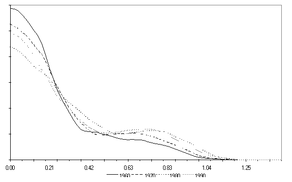
- Pyka/Krüger/Cantner (1999) provide an empirical and theoretical analysis of this issue. Drawing on the Summers/Hestons Penn World Table 5.6 (1991) they determine kernel density distributions which are able to detect the aforementioned twin peaked structure. Figure 1 shows the result found when dealing with per capita incomes; there incomes increase from the left to the right. The distribution of those per capita income levels are shown for the years 1960, 1980 and 1990. Most interestingly the development of these density plots shows that starting with an unimodal structure in 1960 a bimodal or twin-peak structure emerges from 1980 onward.
|
|
Figure 1. Income distribution for selected years ((1999)Pyka/Krüger/Cantner 1999)
|
- 1.3
- In order to explain this development and the especially the emergence of a twin-peak income structure Pyka/Krüger/Cantner (1999) introduce a theoretical model which shows how differences in the ability of countries to improve their technological performance lead to clear separation of technologically leading countries from those which lag behind. Thus, the empirical results obtained can be explained theoretically.
- 1.4
- This paper attempts to extend this discussion by taking the reverse procedure as in Pyka/Krüger/Cantner (1999), that is to find empirical evidence for the working mechanism of the theoretical model. In particular, since the theoretical model is mainly based on so-called transition rates from lower to higher technological levels (and vice versa) we attempt to detect empirically grounded values for the parameters of these transition rates. Applying them to the theoretical model it will be tested whether the mechanism responsible for the theoretical twin-peak structure holds also for the empirically determined bi-modal distribution of per capita incomes.
- 1.5
- We proceed as follows: Section 2 briefly introduces the theoretical model and states the results pertaining to the twin-peak structure. Section 3 describes the construction of the transition rates from the empirical data. The parameters of the theoretical specification is estimated by NLS and plugged into the simulation analysis in section 4. Section 5 introduces a non-parametric estimation technique to estimate both functional form and parameters This procedure is applied to the data and the estimated transition functions are used for simulation. Section 7 concludes.
 Twin-peak structures - the theoretical model
- 2.1
- We are first going to briefly introduce a self-organisation model, originally developed by Cantner/Pyka (1998) in an industrial economics context and applied in Pyka/Krüger/Cantner (1999) to the international distribution and development of per capita incomes or labour productivity.
- 2.2
- As a major determinant for productivity differences and their development we consider the technological know-how of an economy. The accumulated technological know-how depends on (1) the intensive technological opportunities offered by a technological paradigm, (2) the degree by which this opportunity space has already been exhausted and (3) the technological infrastructure, i.e. absorptive capacities, transfer mechanisms influencing this process. To describe the productivity levels of the different countries we draw on the following representation of a relative technological scale in Figure 2.

|
|
Figure 2. Relative technological scale
|
- 2.3
- We apply a scale with n different states or technological levels xi = i/n where i ∈ {1, ... , n}. Each technological state is characterised by the level of accumulated knowledge and a certain degree of technological infrastructure. The assumptions are represented as follows: Productivity levels are cumulatively increasing within this interval. The lowest level x1 represents the productivity level going hand in hand with a common available knowledge stock and is considered as a minimum productivity level always achievable. The most sophisticated technological level, the world technological frontier is xn representing the highest productivity level. Technological infrastructure is also assumed to improve along the technological scale, thereby assuming that with higher technological levels also the technological competencies within the economy increase. This means that for realising lower productivity levels drawing on the common available knowledge stock is more or less sufficient, whereas for higher productivity levels specific capabilities become necessary due to a higher degree of complexity of the respective technologies.
- 2.4
- In order to investigate long-run productivity developments we interpret the scale as a relative one. Consequently, xn is considered as the best practice productivity level at a certain point in time t and the other states xi (i≠n) are to be seen relative to xn. This technological scale allows to model productivity improvements of an economy as movements from state xi to its adjacent neighbour xi+1. Taking into account the intrinsic uncertainty of innovation processes, the probability of an economy to move along the relative technological scale is affected by three determinants:
- the degree of exploitation of intensive technological opportunities
- the effectiveness of the underlying technological infrastructure and
- technological obsolescence.
- 2.5
- These determinants are formalised by means of transition rates. However, before we introduce these main determinants of the model, a few remarks with respect to the synergetic modelling approach applied are necessary.
- 2.6
- The introduced relative technological scale can be interpreted as a discrete state-space on which the economies' productivity levels evolve in time. It is analytically tractable with the so-called master-equation approach. Applying this, the productivity improvement and the respective productivity level achieved by an economy are stochastic. Consequently, the probability to meet a certain productivity level in time t also is a measure for the relative shares of the economies on this productivity level within the whole population.[1]
- 2.7
- Which factors affect these shares/probabilities of a certain state and how do they change? A master equation computes for every single state of the state space the probability to meet this state at a certain point in time t. The basic mechanism of this equation is illustrated in Figure 3.

|
|
Figure 3. Basic mechanism of a master-equation
|
- 2.8
- A specific productivity state xi can be left in every infinitesimal small time interval due to two reasons: on the one hand, economies successfully improve their productivity and reach the higher level xi+1, on the other hand, technological obsolescence can be responsible for an economy to find itself on a lower productivity level xi-1. These movements, indicated by the arrows below the scale, out of the respective state xi decrease its probability. In the same way economies on the lower productivity level xi-1 could increase their productivity and find themselves in the state xi, or firms on the higher level xi+1 fall back on xi because of technological obsolescence. These movements, indicated by the above arrows into state xi, increase its probability. The dotted arrows for the respective border states indicate that these states could be either reached or left only from one direction
- 2.9
- With the above remarks various factors are introduced which influence relative productivity improvement and relative deterioration of productivity levels of an economy. These influences are represented by transition rates between two neighboured states i and j.
Exploitation of intensive technological opportunities

|
|
(1)
|
- 2.10
- (1) describes the probability p of improving from technological level xi to the adjacent level xi+1 (i+1←i) by exploiting the intensive opportunity space.
Technological infrastructure
- 2.11
- The probability of productivity improvements ri+1←i with respect to technological infrastructure formally is as follows:

|
|
(2)
|
- 2.12
- Parameter b represents the difficulty of building up technological infrastructure. The lower this parameter, the sooner and consequently on lower productivity levels positive effects of drawing on external knowledge thereby realising cross-fertilisation effects i.e. exploring new technological opportunities become possible. With a large b the function becomes rather steep in the middle part and sharply separates productivity levels with a developed technological infrastructure from those without. The parameter g ∈ [0, 1] is a kind of sensitivity parameter which determines the minimum amount of technological competencies for the exploration of extensive opportunities. For relatively small values of g a relative low amount of competencies is necessary to build up technological infrastructure. Parameter γ again is a weight.
Technological obsolescence
- 2.13
- We assume a constant obsolescence o representing exogenous determinants. Their impact increases on higher technological levels.. On the technology-scale the rate of obsolescence oi-1←i is modelled by:

|
|
(3)
|
- 2.14
- Thus, technological obsolescence is represented here as a permanent move to the left of the scale: On the right side higher productivity levels enter the opportunity space of economies, on the left side the common available knowledge stock grows and with it the lowest productivity level x1. This provides for that economies will perform at least this productivity level.
- 2.15
- With transition rates (1), (2) and (3) we are now able to formulate the master-equation describing the technological dynamics of the model. The transition-rates only depend on the different states xi and are time-independent. Therefore, we are dealing with a non-stationary Markov-model which looks as follows:[2]

|
|
(4)
|
- 2.16
- To close the system, the border equations for state x1 and xn have to be formulated separately, because they can be reached from and left in only one direction ('reflecting barriers'). For this see Cantner/Pyka (1998).
- 2.17
- The simulation performed in Pyka/Krüger/Cantner (1999) is based on the following specification of the parameters in (1) -(3):
|
| Eq. (1) | α = 0.775 |
| d = 3.5 |
|
| Eq. (2) | g = 0.5 |
| b = 15 |
| γ = 0.225 |
|
| Eq. (3) | o = 0.27 |
|
- 2.18
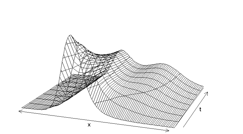
- The simulation of the model is performed for a technological scale with n=100 different productivity levels. This choice of n is sufficient to track interesting developmental aspects. All simulation runs are composed of 10,000 iterations. Furthermore, in the simulation all economies start on the lowest productivity level x1 (common available knowledge stock) (P(x1|0) = 1).The distributions of productivity levels over time are shown in Figure 4.
|
|
Figure 4. Simulated productivity distribution over time
|
- 2.19
- All countries start on the technological level x1 and therefore no differential technological infrastructures exist. The development of this structure is the as follows:
- 2.20
- First, the development leads to an unimodal structure which is characterized by a certain degree of heterogeneity among countries. At this stage and due to the observed heterogeneity among countries the influence of technological infrastructure becomes more and more effective leading to a characteristic twin peaked shape. Finally, we find a clear separation of two groups of countries: a likewise larger group staying continuously on smaller productivity levels, and a small group of leading countries, which are successfully maintaining their high productivity levels.
- 2.21
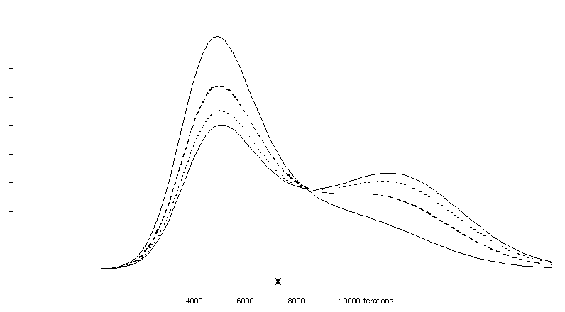
- Figure 5 shows for selected periods the phase portraits of productivity distribution corresponding to Figure 1 above. By comparing these two figures a striking similarity becomes obvious.
- 2.22
- As the choice of the parameters for the simulation was quite arbitrary so objections might be raised arguing that the emerging twin peak structure is due to the choice of the parameters and due to the choice of the functional form in equation (1)-(3). We want proceed in this paper by basing first parameters (section 4) and then functional forms and parameters (section 5) on the observed data.
|
|
Figure 5. Productivity distributions for selected iterations (phase portrait)
|
 Data
Data
- 3.1
- The data set used to quantify the model is real GDP per worker data from the Penn World Table 5.6 (Summers/Heston 1991) for all 104 countries for which a complete time series for the period 1960-90 is available:
.
- 3.2
- These data are first transformed into GDP per worker relative to the USA by dividing the GDP per worker of each country in a particular year by the GDP per worker of the USA in that year:
- 3.3
- Then we classified each country for each year into one of 20 classes according to
- 3.4
- From this classification we constructed the variables pr and o which give estimates of the probabilities that a country that is contained in class i jumps forward to class i+1 or backward to class i-1
where the operator #(.) represents the number of members of a particular class and years for which the argument is true. In the following these probabilities are abbreviated by and for each class. The centers of the 20 classes on the scale [0,1] are given by x, i.e.
.
- 3.5
- In the light of the explanatory power of our regressions we think that 20 classes are a good compromize between the estimation error of the probabilities for each class and the goodness of fit in the regression analysis.
 NLS Estimation of the Theoretical Specification
- 4.1
- With these variables at hand we can estimate the parameters of the equations of the theoretical model in Pyka/Krüger/Cantner (1999) by nonlinear least squares (NLS). Because the log likelihood function suffers from multiple maxima we tried various randomly chosen starting values for the coefficients to find the global maximum of the log likelihood function. This procedure is applied to all regressions for which results are presented in this paper. Because we could not get separate estimates for the p and r functions of the theoretical model we proceeded by using an additive specification of both variables. The results of the NLS estimation are presented in Table 1.
- 4.2
- We observe a surprisingly high value of R2 accompanied by insignificant coefficient estimates as is evident from the t-statistics. This may be an indicator of a multicollinearity problem in this equation. However, our main objective is not to identify each parameter separately but to obtain a well fitting functional form that can be used in the simulation of the master equation in a further step.
|
Table 1: Theoretical Specification:  |
|
| Coefficient | t-Statistic | p-Value |
| β1 (= α) | -0.0783 | -0.2647 | 0.7949 |
| β2 (= -d) | 2.3486 | 0.8586 | 0.4041 |
| β3 (= γ) | 0.7895 | 0.8317 | 0.4186 |
| β4 (= b.g) | -1.7279 | -0.5203 | 0.6104 |
| β5 (= -b) | -4.4012 | -0.1079 | 0.9155 |
 | 0.9000 | | |
| ln L | 45.7433 | | |
| Note: t-statistics and p-values are based on heteroskedasticity consistent standard errors |
|
- 4.3
- Table 2 contains the results for the obsolescence equation which shows a highly significant coefficient estimate and a not too bad fit to the data.
|
Table 2: Theoretical Specification:  |
|
| Coefficient | t-Statistic | p-Value |
| φ1 (= 0) | 0.2296 | 6.7165 | 0.0000 |
 | 0.3004 | | |
| ln L | 27.4072 | | |
| Note: t-statistics and p-values are based on heteroskedasticity consistent standard errors |
|
- 4.4
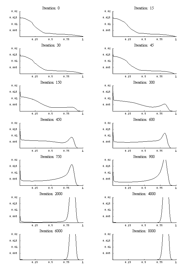
- Using these empirically determined transition rates in the master equation already applied in section 2 we run again a simulation. Figure 6 shows the structure of the income distribution for selected numbers of iterations. We start with the income distribution of the year 1960 as estimated by kernel density techniques. This figure clearly shows the estimated theoretical specification is able to replicate the twin peaked structure only as a transitory phenomenon, whereas in the long-run a single peaked distribution shows up.
|
|
Figure 6. Simulation results of the theoretical specification
|
- 4.5
- This result of only transitory emerging twin peaks may be caused by the particular functional forms chosen for the transition rates in the theoretical model. The question arising is whether other functional forms can be identified without strong a priori assumptions as needed for a parametric specification. In the following step we want to generate both the functional form and the parameters form the observed data.
 The functional search algorithm
- 5.1
- The functional algorithm bases on the genetic programming approach recently introduced by Koza (1992) to solve complex optimization problems by means of simulating evolution. A small collection of genetic programming applications in realm of economics can be found in Koza (1992) and Schmertmann (1996)[3]. The properties of the functional search algorithm when used in empirical analysis in economics are analyzed in Ebersberger/Cantner/Hanusch (2000). In particular they show that the functional search algorithm maintains a non-parametric approach to discover a functional relationship buried in the data. Hence it does not wed the data with some ex ante specified model rather lets it speak the data for itself.
- 5.2
- The functional search algorithm belongs to a class of evolutionary algorithms. Generally speaking it simulates evolution as to breed a perfect or sufficiently good solution to a predefined problem. The functional search algorithm in particular constructs a sequence of populations each containing a number of candidate functions that describe the empirical data. Applying Darwinian operators and simulating evolution on the populations increases their overall quality in portraying the data. The best candidate function in the final population of the evolution is the result of the functional search.
- 5.3
- To start the search process we first generate a random population of a large number of individual functions. Those functions are evaluated on how good they approximate a given data set and are assigned a real number accordingly. This number indicates the fitness of the individual candidate function - in our set up here we choose a simple R2 as a fitness measure of the individual candidate function. The next generation is created by selecting the candidate functions based on their fitness and applying genetic operators, such as crossover and mutation, before they enter the new generation. Any individual function in this generation is again evaluated on how good it portrays the data. The best functions are selected and transformed to enter the successive generation .... and so forth. By repeating this procedure for several(-hundred) generations the fitness of the best individual function in the generation improves and a solution to the functional search problem emerges. The basic idea ruling the algorithm is the hypothesis that good individuals are built from good components (building blocks, schema) and the recombination of those good building blocks leads to even better building blocks, creating ever improving individuals in the course of time. A detailed exposition of the algorithm can be found in Ebersberger/Cantner/Hanusch (2000).
- 5.4
- The technical specification of the algorithm we applied to the data set discussed in section 3 can be seen from Table 3.
|
| Table 3: Specification of the Functional Search Algorithm |
|
| Characteristic | Default value |
| objective | find functional form and parameters simultaneously for o(x) and pr(x) |
| number of individuals in population | 200 |
| set of primitive functions | +, -, /, *, ^, exp |
| set of terminals | Constants c drawn from [0,1], x |
| fitness function (to be maximized) | R2 |
| termination criterion | Number of generations > 200 |
| genetic operators | Subtree-mutation, subtree-crossover, copying of the best individual, reproduction |
| |
|
- 5.5
- As can be seen from Table 3 we used a standard set up of the functional search algorithm that we implemented in MATHEMATICA 4. However some peculiarities are worth mentioning: First, we used brood-crossover (Tackett 1994) to improve the computational efficiency of the algorithm. Second, we used a parsimony pressure term suggested by Zhang and Mühlenbein (1995) to supplement the fitness function to guide the algorithm towards accurate and parsimonious solutions.
- 5.6
- Running the functional search algorithm on the data set produced resulted the following functional forms:
- 5.7
- To improve upon the result of the functional search we maintained the functional form of the results and substituted the numerical values (1.5763, 0.2003, 0.6206) with parameters (θ1, δ1, δ2) to be estimated by NLS. Tables 4 and 5 show the estimation results.
|
Table 4: Empirical Specification:  |
| Coefficient | t-Statistic | p-Value |
| θ1 | 1.5453 | 32.5218 | 0.0000 |
 | 0.9026 | | |
| ln L | 43.6456 | | |
| Note: t-statistics and p-values are based on heteroskedasticity consistent standard errors |
|
|
Table 5: Empirical Specification:  |
|
| Coefficient | t-Statistic | p-Value |
| δ1 | 0.1936 | 4.5565 | 0.0002 |
| δ2 | 0.5235 | 2.4320 | 0.0257 |
 | 0.4066 | | |
| ln L | 29.5940 | | |
| Note: t-statistics and p-values are based on heteroskedasticity consistent standard errors |
|
- 5.8
- These differ considerably from the functions postulated by Pyka/Krüger/Cantner (1999). They are less heavily parameterized as the theoretical specification and contain coefficient estimates that are different from zero on usual significance levels. The fit of the pr equation is not worsened in this more parsimonious specification and the fit of the o equation has improved considerably.
|
|
Figure 7. Simulation results of the empirical specification
|
- 5.9
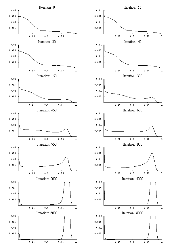
- Simulation of the master equation using the functional form obtained from genetic programming, leads to the structural development as depicted in Figure 7. If we compare this development with the one graphed in Figure 6 we detect no striking difference up until iteration 900. A bimodal distribution emerges. Beyond iteration 900 both setups start to develop different structures. The simulation based on the empirical specification maintains the bimodal structure of the distribution whereas the theoretical specification yields the bimodal shape as a transitory phenomenon.
Conclusion
- 5.10
- So what have we learned from this exercise? For understanding the twin-peaked distribution of national income per capita a synergetic model based on the master equation approach has proved to be useful. Starting point of our investigation was the empirical distribution function estimated by a nonparametric kernel density estimator. Here we observed the evolution of the national income distribution from a unimodal one in 1960 toward a bimodal distribution in 1990. The essential qualitative features of this development can be replicated by the specification of and parameter choice for the transition rates used to implement the master equation approach as suggested by Cantner and Pyka (1998) and Pyka, Krüger and Cantner (1999). Since the parameter choice in these papers was purely ad hoc, in the present paper we bring the model and the data more close together.
- 5.11
- For this we proceeded in two steps. In the first step we took over the postulated functional forms of the theoretical model and estimated the parameter values by NLS using data from the Penn World Table. These regressions fitted the data quite well and the following simulation of the model starting from the 1960 distribution produced a bimodal shaped distribution for a certain amount of simulated periods but the ergodic distribution did no share this feature. In such a highly stylized model, there is always a large amount of specification uncertainty caused by the need to choose specific functional forms. Therefore, in the second step dispensed with the assumed functional forms of the transition rates of the theoretical model. One appropriate way to find parameterized functional forms from a data set nonparametrically is the method of genetic programming. This lead by and large to a considerably more parsimonious specification of the transition rates that was accompanied by a slightly improved overall fit. In contrast to the earlier simulation of the model with these alternative transition rates produced a twin-peaked ergodic distribution.
- 5.12
- In our opinion the approach employed in this paper is very useful in reducing the present distance of most simulation models to real world phenomena. Its central feature lies in the ability to 'find' a parametrically specified functional form that fits best to the data without restricting this functional form to a certain class or family. So the traditional purely ad hoc procedure of examining various chosen functional forms is augmented by a procedure to uncover the form of functional relationships directly from the data without employing too much a priori knowledge.
 Notes
Notes
-
1 See e.g. Honerkamp (1989).
2 For a detailed formal description of the model see Cantner/Pyka (1998).
3 The term functional search dates back to Schmertmann (1996) whereas Koza (1992) speaks of symbolic regression. Kargupta and Sarkar (1999) use the term function induction for a related procedure. We do not want to insinuate that functional search is used as a purely inductive device of analysis nor do we want to get confused with traditional regression analysis, hence we refer to the methodology as functional search as to stress the search-like character of the procedure.
 References
-
ABRAMOVITZ, M. (1986), Catching Up, Forging Ahead and Falling Behind, Journal of Economic History 46, 1986, 385-406.
BAUMOL W.J. (1986), Productivity Growth, Convergence and Welfare: What Long Run Data Show, American Economic Review 76, 1986, 1072-85.
CANTNER, U., PYKA, A. (1998), Technological Evolution - An Analysis within the Knowledge-based Approach, Structural Change and Economic Dynamics 9, 1998, 85-108.
EBERSBERGER, B., CANTNER, U., HANUSCH, H. (2000), Functional Search in Complex Evolutionary Environments - Examining an Empirical Tool, in: Rakotobe-Joel, T. (ed) Complexity and Complex Systems in Industry, Warwick 2000, forthcoming.
FAGERBERG, J. (1988), Why Growth Rates Differ?, in: Dosi G., C. Freeman, R. Nelson, G. Silverberg, L. Soete (eds), Technical Change and Economic Theory, London: Pinter, 1988, 432-57.
HONERKAMP, J. (1989), Stochastische dynamische Systeme: Konzepte, numerische Methoden, Datenanalysen, VCH-Verlagsgesellschaft, Weinheim.
KARGUPTA, H., SARKAR, K. (1999), Function induction, gene expression, and evolutionary representation construction, in W. Banzhaf, J. Daida, A. E. Eiben, M. H. Garzon, V. Honavar, M. Jakiela and R. E. Smith (eds), Proceedings of the Genetic and Evolutionary Computation Conference, Vol. 1, Morgan Kaufmann, Orlando, Florida, USA, pp. 313-320.
KOZA, J. (1992), Genetic Programming: On the Programming of Computers by Means of Natural Selection, MIT Press, Cambridge, MA.
KRÜGER, J.J., CANTNER, U., HANUSCH, H. (2000), Total Factor Productivity, the East Asian Miracle and the World Production Frontier, Weltwirtschaftliches Archiv 136, 111-136
NELSON, R.R., PACK, H. (1999), The Asian Miracle and Modern Growth Theory, Economic Journal 109, 1999, 416-436.
PACK, H., PAGE, J.M. (1994), Accumulation, Exports, and Growth in the High-Performing Asian Economies, Carnegie-Rochester Conference Series on Public Policy 40, 1994, 199-236.
PYKA, A., KRÜGER, J.J., CANTNER, U. (1999), Twin-Peaks - What the Knowledge-Based Approach Can Say About the Dynamics of the World Income Distribution, University of Augsburg, Department of Economics Discussion Paper No. 189, 1999.
SCHMERTMANN, C.P. (1996), Functional search in economics using genetic programming, Computational Economics 9, 275-298.
SUMMERS, R., HESTON, A. (1991), The Penn World Table (Mark 5): An Expanded Set of International Comparisons 1950-1988, Quarterly Journal of Economics 106, 1991, 327-368.
TACKETT, W.A. (1994), Recombination, Selection, and the Genetic Construction of Computer Programs, PhD thesis, University of Southern California, Department of Electrical Engineering Systems.
VERSPAGEN, B. (1991), A New Empirical Approach to Catching Up or Falling Behind. Structural Change and Economic Dynamics 2, 1991, 359-380.
VERSPAGEN, B. (1992), Uneven Growth Between Interdependent Economies - An Evolutionary View on Technology Taps, Trade and Growth, Maastricht: Universitaire Pers Maastricht, 1992.
WORLD BANK (1993), The East Asian Miracle: Economic Growth and Public Policy, New York: Oxford University Press, 1993.
ZHANG, B.T., MÜHLENBEIN, H. (1995), Balancing accuracy and parsimony in genetic programming, Evolutionary Computation 3, 17-38.

 Return to Contents of this issue
© Copyright Journal of Artificial Societies and Social Simulation, 1999
 Abstract
![]() Introduction
Introduction
![]() Twin-peak structures - the theoretical model
Twin-peak structures - the theoretical model


![]()
![]()
![]()


![]() Data
Data![]()


![]()
![]() NLS Estimation of the Theoretical Specification
NLS Estimation of the Theoretical Specification


![]() The functional search algorithm
The functional search algorithm


![]() Notes
Notes![]() References
References![]()
Return to Contents of this issue